Computational Issues Related to the Discrete Wavelet Analysis of Power Systems Ileana-Diana V.D. Nicolae*, Petre-Marian T. Nicolae**, Dorina-Mioara C. Purcaru*** *Department of Computers and Information Technology (e-mail:
[email protected]) **Department of Electrical Engineering, Power Systems and Aeronautics (e-mail:
[email protected]) ***Department of Automation, Electronics and Mechatronics (e-mail
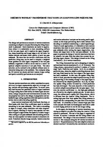
[email protected]) University of Craiova, Decebal Blv. No. 107 Abstract: The paper is dedicated to computational aspects related to the Discrete Wavelet Transform use for the analysis of electric signals in power systems. The most important aspects considered when selecting the analysis method are related to the use of proper techniques, able to avoid (or at least to limit as much as possible) the obtaining of inaccurate results because the applied theoretical algorithms assume signals of infinite length whilst only finite segments of them are submitted to the computational process at a specific moment. One intends to obtain reliable power quality indices (with minimum deviations from those calculated with the Fast Fourier Transform) and non-(or minimum) delayed, non-ambiguous “response” of details vectors to disturbances. The avoiding of fake faults detection or of real ones’ missing, owing to the “edge effect”, along with other important aspects concerning the real-time operation (execution time and memory consumptions) were also considered. Keywords: Signals processing, Wavelet Analysis, Quality in power systems. 1. INTRODUCTION When the Discrete Wavelet Transform (DWT) is used to perform a Multi-resolution Analysis (MRA), firstly the original waveform S is decomposed in approximations and details. Afterward successive decompositions of the approximations are made, with no further decomposition of the details. Fig.1, depicts a decomposition on 3 levels (Nicolae I.D. and Nicolae M.S. (2011), Mallat, S. (1998)). cAi denotes the approximation vector whilst cDi denotes the detail vector on the i-th level. The most significant frequencies from the original signal appear with high magnitudes in that specific region of the DWT signal including them, with the preservation of their time localization. Power quality is a permanent concern nowadays, continuous efforts being done to find more efficient methods for its analysis (Manjunath, A., Ravikumar , H.M. (2010)).
For the analysis of distorting regimes, the Discrete Wavelet Transform is a valuable tool. Preliminary evaluations are required in order to determine the proper Wavelet mother order and the proper number of levels from the decomposition tree. When the determination of power quality indices is intended, criteria like minimum energy deviations and respectively minimum approximation error generated by the signal recomposition process yield reliable results. The Fast Fourier Transform can be used for steady regimes in order to provide “reference data” for the values obtained for power quality indices when DWT-based theories are used (Nicolae, I.D. and Nicolae, P.M. (2011)). 2. MATHEMATIC AND COMPUTATIONAL ISSUES 2.1 Techniques to avoid the edge effect When handling signals with finite length, in order to deal with border distortions, the border should be treated differently from the other parts of the signal (Bastis, A. (2003)). Various methods are available to deal with this problem, referred to as "wavelets on the interval" (Cohen et al, 1993). These interesting constructions are effective in theory but are not entirely satisfactory from a practical viewpoint (Misiti, M. et al 2007, Matlab documentation).
Fig. 1. A decomposition on 4 levels using DWT
Details on the rationale of these schemes are presented by Strang and Nguyen (1996).
In Matlab, the available signal extension modes (usable by means of the option “dwtmode” of the polymorphic function “dwt”) are as follows :
One step of the forward transform can be expressed as the infinite matrix of wavelet coefficients represented below, multiplied by the infinite signal vector (s).
Zero-padding ('zpd'): This method assumes that the signal is zero outside the original support. The disadvantage of zero-padding is that discontinuities are artificially created at the border.
ai
=…h0, h1, h2, h3,0,0,0,0,0,0,0,0…
si
ci
=… l0, l1, l2, l3, 0,0,0,0,0,0,0,0…
si+1
ai+1
=…0,0,h0, h1, h2, h3,0,0,0,0,0,0…
si+2
Symmetrization ('sym') –default option. This method assumes that signals or images can be recovered outside their original support by symmetric boundary value replication. Symmetrization has the disadvantage of artificially creating discontinuities of the first derivative at the border (works well in general for images).
ci+1
=…0,0,l0, l1, l2, l3,0,0,0,0,0,0,…
si+3
ai+2
=…0,0,0,0,h0, h1, h2, h3,0,0,0,0,…
si+4
ci+2
=…0,0,0,0,l0, l1, l2, l3,0,0,0,0,0,…
si+5
ai+3
=…0,0,0,0,0,0,h0, h1, h2, h3,0,0,…
si+6
ci+3
=…0,0,0,0,0,0,l0, l1, l2, l3,0,0,…
si+7
Smooth padding of order ('spd' or 'sp1'). This method assumes that signals or images can be recovered outside their original support by a simple first-order derivative extrapolation: padding using a linear extension fit to the first two and last two values. Smooth padding works well in general for smooth signals. Smooth padding of order 0 ('sp0'). This method assumes that signals or images can be recovered outside their original support by a simple constant extrapolation. For a signal extension this is the repetition of the first value on the left and last value on the right. Periodic-padding, fist version ('ppd'). This method assumes that signals or images can be recovered outside their original support by periodic extension. The disadvantage of periodic padding is that discontinuities are artificially created at the border. The DWT associated with these five modes is slightly redundant. But IDWT (the inverse function for DWT) ensures a perfect reconstruction for any of the five previous modes whatever the extension mode used for DWT. Periodic-padding 2-nd version ('per'): If the signal length is odd, the signal is first extended by adding an extra-sample equal to the last value on the right. Then a minimal periodic extension is performed on each side. This mode produces the smallest lenghtwave decomposition. Often it is preferable to use simple schemes based on signal extension on the boundaries. This involves the computation of a few extra coefficients at each stage of the decomposition process to get a perfect reconstruction. The extension is needed at each stage of the decomposition process. 2.2 An algorithm for real-time implementations Some algorithm-related problems considered during the implementation of a fast direct DWT function, with high/low filters consisting in 4 coefficients (Jensen, A. and Cor-Harbo, A., (2001)) are described below. This function exhibited features that allow it to provide reliable results for the real-time analysis of electric signals in power plants. The coefficients for the scaling function are denoted as hi (high) and the wavelet coefficients are denoted as li (low).
The dot product (inner product) of the infinite vector and a row of the matrix produces either a smoother version of the signal (ai) or a wavelet coefficient (ci). In an ordered wavelet transform, the smoothed coefficients ai are stored in the first half of an n element array region. The wavelet coefficients (ci) are stored in the second half of the region with n elements. The algorithm is recursive (the smoothed values become the input to the next step). The transpose of the forward transform matrix above is used to calculate an inverse transform step. Here the dot product is formed from the result of the forward transform and the inverse transform matrix row, as explained below. si
=…h2, l1, h0, l0,0,0,0,0,0,0,0,0…
ai
si+1
=… h3, l3, h1, l1, 0,0,0,0,0,0,0,0…
ci
si+2
=…0,0, h2, l1, h0, l0,0,0,0,0,0,0…
ai+1
si+3
=…0,0, h3, l3, h1, l1,0,0,0,0,0,0,…
ci+1
si+4
=…0,0,0,0, h2, l1, h0, l0,,0,0,0,0,…
ai+2
si+5
=…0,0,0,0, h3, l3, h1, l1,0,0,0,0,0,…
ci+2
si+6
=…0,0,0,0,0,0, h2, l1, h0, l0,,0,0,…
ai+3
si+7
=…0,0,0,0,0,0, h3, l3, h1, l1,0,0,…
ci+3
Using a standard dot product is inefficient since “sparse” matrices are involved. In practice the wavelet coefficient values are moved along the signal vector and a four element dot product is calculated. Expressed in terms of arrays, for the forward transform this would be: ai = s (i ) * h0 + s (i + 1) * h1 + s (i + 2) * h2 + s (i + 3) * h3 ci = s (i) * l0 + s (i + 1) * l1 + s (i + 2) * l 2 + s (i + 3) * l3
(1)
When applied to a signal with the length N, if i=N-1, the elements with indices i+2 and i+3 will be beyond the end of the array. The version of the algorithm used for our implementation assumes that data is periodic, than data at the start of the signal wraps around to the end. The reconstruction features of the pair of functions that we have written in Matlab to implement the above algorithm were tested on several signals (gathered with a specialised data acquisition system). The results confirmed
Table 1. Values for percent deviations of power quality indices, calculated with dwt - different options, reported to the power indices calculated with dwm
Fig. 2. Reconstruction error the reproducibility features (Fig. 2), as in all the cases the reconstruction error did not exceed the value of 10-12 (which is more then 14 orders of magnitude smaller than the decomposed signal). 3. OPERATIONAL CONTEXT AND PRELIMINARY EVALUATIONS Our original program was implemented on a desktop running Matlab vers. 7.1 under Windows XP, personalised to run for „best performances”. The main characteristics of the computer are: processor’s frequency of 2.4 GHz and 2GB of RAM. The data acquisition system (with 8 channels) was set to supply samples with a sampling rate which is small enough (almost 560 samples/periode) such as to allow one to deduce a comprehensive set of information on the acquired data, in an ASCII form, as „quanta” . It means that the data needs more processing, as the mean value of the quasi-sinusoidal is not zero (as it should be), because a certain displacement relative to the Oy axis is introduced by the system. Therefore a „calibration to 0” operation was done firstly. The signal selected for the comparative studies has distorsions, being typical for stationary regimes in power systems. It is depicted by Fig. 3. As the method used for the DWT analysis must provide reliable power quality indices, we made comparative studies on results obtained with our function (implementing the algorithm described in the 2-nd section) and respectively with dwt provided by Matlab, for the same values of filters and different values
Percent deviations Ij0 Ijn I 1.3663 -5.2441 1.0220 -13.6858 -27.9354 -14.4477 -13.6635 -8.4964 -13.4083 2.6662 -54.1853 -0.9742 1.3179 -5.5025 0.9623 1.9287 -29.7846 0.0860 -5.6784 -7.6127 -5.7769 -12.7914 -7.5739 -12.5338 0.7574 -13.3051 0.0000
Setting of dwtmode spd sym(h) symw asym(h) asymw zpd ppd sp0 per
for the option “dwtmode”. Table 1 gathers the percent relative differences between the values calculated with dwt (dwtmode as mentioned in the 1-st column) and the value calculated with our function (we will refer our method as “dwm”). The compared values were: the “node-zero” current, the “non-zero node“ current and the current’s RMS value respectively. The following expression for the current’s RMS value was used (Morsi, W.G. and El-Hawary, M.E. (2009)): I=
1 T
T
∫
0
i 2 (t )dt =
1 T
∑c k
2 jO ,k
+
1 T
∑∑ d j ≥ jO k
2 j ,k
= I 2jO +
∑I
2 j
(2)
j ≥ jO
Ij0 denotes the RMS value for the band with the lowest frequency j0. It is also called „approximate” current or the “node zero” current. Ij represent the sets of RMS values for higher frequency bands (also called “detail” currents Idet). Their sum gives the so-called “non-zero node” currents. cj0,k are the discrete wavelet coefficients, for the scale j0, and sample k, whilst dj,k are the discrete wavelet coefficients for the level j≠ j0, sample k : c jO , k = 〈 v(t ), φ jO , k 〉 , d j , k = 〈 v(t ), ψ j , k 〉 ,
(3)
In the above equation φj0,k represents the scale, ψj,k represents the wavelet function and „< >” is used to represent the scalar product. The results calculated with dwm are: Ij0=462.3985A, Ijn=106.6238 and I=474.5324. Considering that the maximum value of the signal is 653.136 A and therefore, a perfect sine-wave with the same magnitude should have a RMS value of 461.8369A, it is obvious that dwm provides a correct evaluation of the considered indices (as it does not introduce any artificial enlargement of the decomposition vectors). Moreover, the fft analysis of the considered signal revealed differences lower then 1.2% . The percent differences from Table 1 were calculated with: (val _ dwm − val _ dwt ) / val _ dwm × 100
Fig. 3. Analysed signal
(4)
To avoid the „artificial enflating” of the signals energies introduced at each step by dwt (all options excepting „per”), we eliminated the final part from the vectors (artificially introduced by the dwt algorithm, as described
in Section 4). This technique improves the accuracy of power-related indices’ evaluation, but makes more difficult the recomposition of the original signal from its decomposition vectors (as idwt can no longer be used). Our previous researches (Nicolae, I.D. et all, unpublished (2011)) considering the abilities of dwt to detect in an undelayed manner the faults or to detect the real faults near the signal edges and respectively not to detect fake defaults owing to the Gibs phenomenon, along with the (expected) results from Table 1, resulted into the selection of only two modalities for the use of dwt: with dwtmode=’spd’, respectively with dwtmode=’per’. 4. USING DWT WITH SMOOTH PADDING
Fig. 6. Stationary. dwt (smooth padding) vs dwm, decomposition at 10-th level
4.1. Analysis with smooth padding, stationary regime Our simulations were firstly concerned with a comparative analysis of the results obtained for a decomposition made on 10 levels, a number of 4096 points/period. We used dwm and respectively dwt with dwtmode=’spd’. Some results are depicted by Fig. 4-6 (green – dwm, black - dwt). At each level, unlike dwm, the Matlab algorithm introduces new points at the end of the decomposition vectors, as one can see in Fig. 4-6 (marked by ellipses).
Fig.7. Stationary. dwt (smooth padding) vs dwm, energies of levels The energies of the decomposition vectors versus levels are depicted by Fig.7, the mean values of the approximations can be seen in Fig. 8, whilst the mean values of the details can be seen in Fig. 9.
Fig. 4. Stationary. dwt (smooth padding) vs dwm, decomposition at 6-th level
Fig. 5. Stationary. Smooth padding, dwt and dwm, decomposition at 9-th level
All these figures reveal that an artificial energy is introduced by the Matlab dwt algorithm with smooth padding and its effects are imperfectly reduced by a simple shortening procedure of the vectors’ final newly introduced positions at each level. The mean values are affected, mostly at details, which must be consulted to
Fig.8. Stationary. dwt (smooth padding) vs dwm, mean values of approximations (per levels)
(a) (b) Fig. 11. dwt (smooth padding) vs dwm in non-stationary regime. Zoom for details - 1-st level (a) and 4-th level (b) Fig.9. Stationary. dwt (smooth padding) vs dwm, mean values of details versus levels detect possible faults. The drawback of the shortening procedure in order to get better energetic equivalence with results yielded by FFT are explained in the next section.
5. USING DWT WITH PERIODIC PADDING Fig. 12-14 depicts the results of the comparative analysis “dwt (periodic padding)” versus dwm in stationary regime.
The undesired de-synchronization between the original signal and the dwt’s approximation on the final level is another inconvenient. 4.2. Analysis with smooth padding, regime with randomly induced fault To test the abilities related to faults’ detection exhibited by the decomposition vectors generated with dwt (smooth padding) versus those of the decomposition vectors generated by dwm, we disturbed (through soft) the signal analysed in steady state with a randomly generated signal, as depicted by Fig. 10 (the same colouring convention was used).
Fig.12. Stationary. dwt (periodic padding) vs dwm, decomposition on 6-th level
As revealed by Fig. 11, at the first levels the details have almost synchronous moments for the correct detection of a fault, whilst at higher levels, dwt denotes the default later (incorrectly) – as marked by the circle ‘2’. dwm behaves correctly (circle ‘1’). The “enlargement” introduced by dwt when no “shortening” measures are explicitly taken can be seen in circle ‘3’.
No artificial enlargements of the decomposition vectors were noticed when calling dwt with dwtmode=’per’. The shape of the details is almost the same and the level energies are identical. The mean values of the approximations were also found to be identical at both methods.
Fig.10. Non-stationary. dwt (symmetric padding) vs dwm, 1-st level decomposition of the randomly disturbed signal
Fig.13. Stationary. dwt (periodic padding) vs dwm, decomposition on 10-th level
The analysis with dwt (periodic padding) generates two drawbacks: the major one is related to the difference in details’ energies. They “make the difference” to the
6. CONCLUSIONS
Fig.14. Stationary. Periodic padding dwt and dwm, mean values of details versus levels real power quality indices. Another drawback consists in the phase-difference of the original signal and the approximated vector at higher level. To these drawbacks, another one is added, related to the delaying in detecting a fault (the same that was discussed in the previous section), as depicted by Fig. 15.
The built-in functions of the Matlab’s toolkit dedicated to DWT analysis are not always the best options for a proper analysis of waveforms from power systems. They may induce artificial energies, unacceptable for power quality analysis, may introduce supplementary memory consumption or detect latter the faults. Phase-differences between the approximation vectors and original signal can also occur. Better and faster algorithms can be implemented to provide an improved analysis. The function proposed in this paper does not generate longer decomposition vectors, detects correctly the moment when a fault occurrs, can calculate the RMS value in non-stationary regimes for which FFT is hard to apply in real-time restrictions and exhibits an execution time 10…20 times shorter than that required for the use of DWT in the analysed scenarios. ACKNOWLEDGMENT The work was supported by CNCSIS-UEFISCDI, PN II IDEI Program, code number 536/2008 (contract no. 695/2009). REFERENCES
(a)
(b)
Fig. 15. Periodic padding dwt versus dwm in nonstationary regime. Zoom on details - 1-st level (a) and 4-th level (b) 5. USING ORIGINAL DWT DECOMPOSITION TO DETECT FAULTS The abilities in detecting faults of the dwm are depicted by Fig. 16, which shows the details’ reaction when the analysed signal is randomly disturbed. The value of the RMS over the affected periods is also calculated with dwm and correctly was revealed to be lower than the value from the stationary regime (the disturbance consisted in a randomly generated sequence, subtracted from the original signal).
Fig. 16. Analysis with dwm. The details detect correctly the moment when a disturbance appears
Bastis, A. (2003) The Gibbs phenomenon bounds in wavelet approximations, Proceedings of International Conference on Image Processing, ICIP 2003, vol.1 I 1017-20. Cohen,A., Daubechies I., Jawerth, B. and Vial, P., (1993) Multiresolution analysis, wavelet and fast wavelet transform of an interval, pp.417-421, CRAS, Ser. A, T. 316, Paris. Jensen, A., Cor-Harbo, A., (2001), Ripples in Mathematics. The Discrete Wavelet Transform, Springer Verlag. Mallat, S. (1998), A wavelet tour of signal processing, Academic Press, New York. Matlab doc., available on line at: http://www.mathworks.com /help/toolbox/wavelet/ug/f8-25097.html. Misiti, M., Y. Misiti, G. Oppenheim, J.-M. Poggi (2007), Wavelets and their applications, ISTE DSP Series. Manjunath, A., Ravikumar , H.M. (2010), Comparison of Discrete Wavelet Transform (DWT), Lifting Wavelet Transform (LWT) Stationary Wavelet Transform (SWT) and S-Transform in Power Quality Analysis, Europ. Journ. of Scientific Research, 39, 4, pp.569-576. Morsi, W.G., El-Hawary, M.E. (2009) Wavelet Packet Transform-Based Power Quality Indices for Balanced ad Unbalanced Three-Phase Systems under Stationary and Non-stationary Operating Conditions, IEEE Trans. on Power Delivery, vol. 24, no. 4, pp. 2300-2310. Nicolae, I.D. et all , unpublished (2011) Final report of the grant 695/2009. Nicolae, I.D. and Nicolae M.S. (2011) Using Wavelets to Define and Detect Harmonic Fingerprints in NonSinusoidal Waveforms, Proceedings of SOFTCOM 2011, 19-th International Conf. on Software Telecomm. and Computer Networks, Split-Hvar-Dubrovnik Croatia, SYM 2/III - 75923 – 1609. Nicolae, I.D. and Nicolae, P.M. (2011) Using Wavelet Transform for the Evaluation of Power Quality in Distorting Regimes, Acta Electrotechnica, vol. 52, no.5, pp. 331-338. Strang, G. and Nguyen,T. (1996), Wavelets and filter banks, ed. Wellesley Cambridge Press, Cambridge.