A NESTED COMPUTATIONAL APPROACH TO THE DISCRETE-TIME

A NESTED COMPUTATIONAL APPROACH TO THE DISCRETE-TIME FINITE-HORIZON LQ CONTROL PROBLEM GIOVANNI MARRO?

DOMENICO PRATTICHIZZO‡

ELENA ZATTONI?

? DIPARTIMENTO

DI ELETTRONICA, INFORMATICA E SISTEMISTICA ` DI BOLOGNA, VIALE RISORGIMENTO, 2 – 40136 BOLOGNA, ITALY UNIVERSITA TEL: +39 051 2093046 – FAX: +39 051 2093073 {GMARRO, EZATTONI}@DEIS.UNIBO.IT ‡ DIPARTIMENTO DI INGEGNERIA DELL’INFORMAZIONE ` DI SIENA, VIA ROMA, 77 – 53100 SIENA, ITALY UNIVERSITA TEL: +39 0577 234609 – FAX: +39 0577 233602 [email protected]

Abstract. A new algorithmic setting is proposed for the discrete-time finite-horizon LQ optimal control problem with constrained or unconstrained final state, no matter whether the problem is cheap, singular or regular. The proposed solution, based on matrix pseudoinversion, is completed and made practically implementable by a nesting procedure for welding optimal sub-arcs that enables arbitrary enlargement of the control time interval. Key words. linear-quadratic problems, algorithms, discrete-time systems, pseudoinversion. AMS subject classifications. 49N05, 49N10, 93C05, 93C62

1. Introduction. The LQ and LQR optimal control problems have been extensively studied and are now well settled in the literature. In particular, the regular LQ and LQR problems are exhaustively treated in many well-known specialist books and textbooks, as, for instance, those by Bryson and Ho [3], Kwakernaak and Sivan [12], Anderson and Moore [1], Chen and Francis [5], Lewis and Syrmos [13]. Due to increasing interest in H2 and H∞ control problems, more recently much effort has been made to extend the solutions of LQ and LQR problems also to cheap and singular cases. In general, these new contributions concern the infinite-horizon problems, where optimality jointly with internal stability is required. The basic properties and algorithms referring to cheap and singular optimal control have been investigated by Arnold and Laub in [2], Van Dooren in [23], Ionescu, Oar˘ a and Weiss in [11, 10, 9], Geerts in [6], Saberi, Sannuti, Chen and Stoorvogel in [17, 18, 4, 22] and Soethoudt, Trentelman and Ran in [21, 16]. Extension to cheap and singular problems is obtained by using matrix pencils or linear matrix inequalities. The above contributions mainly refer to continuous- or discrete-time infinite horizon LQR problems. Conversely, this work focuses on the finite-horizon case for discrete-time systems. It applies to cheap, singular or regular problems. Considering a sharp constraint on the final state, this paper extends the results given in [16], where the infinite horizon case with asymptotic endpoint constraints is investigated. However, in the present paper the requirement that the cost functions are positive semidefinite is still present, while in [16] it is not. From the algorithmic viewpoint, the present work differs from those of the abovementioned papers, and is inspired by the system structure algorithm introduced by Silverman in his well known contribution [20], see also [19, 8]. In the present work the solution is achieved by the straightforward technique of pseudoinverting a particular system matrix as in [20], but the time interval considered can be arbitrarily enlarged through a suitable multi-level computational scheme: this enables overcoming any dimensionality constraint, thus achieving a certain interest with respect to 1

2

G. MARRO, D. PRATTICHIZZO and E. ZATTONI

computational practice. The following notation will be used: Rn stands for the set of all n-tuples of real numbers, A0 and A# are used for the transpose and pseudoinverse of matrix A, respectively, and I for the identity matrix with a suitable dimension. 2. Statement of the problem. Consider the linear discrete time-invariant dynamical system (2.1)

x(k + 1) = A x(k) + B u(k) , e(k) = C x(k) + D u(k) ,

x(0) = x0 ,

with x ∈ Rn , u ∈ Rp , e ∈ Rq , k ∈ [0, N − 1], the cost function (2.2)

J :=

N −1 X

e(k)0 e(k) + x(N )0 Z 0 Z x(N ) ,

k=0

and the constraint on the final state (2.3)

G x(N ) = yf ,

yf ∈ R r .

Constraint (2.3) is assumed to be feasible, i.e. the initial state x0 , the constraint on the final state (G, yf ) and the number of steps N of the control time interval are assumed to be such that at least one N -step state trajectory from x0 to an x(N ) satisfying eq. (2.3) exists. It is worth noting that the final state can be completely assigned by assuming G = I in eq. (2.3): in this case the terminal cost becomes irrelevant to the problem solution and in eq. (2.2) matrix Z can be assumed to be zero. On the other hand, assumptions G = 0 and yf = 0 correspond to consider the final state as completely free. The discrete-time finite horizon LQ optimal control problem with constrained final state can be stated as follows. Problem 1. Consider the dynamic system (2.1) and find a control sequence 1 u(k) (k = 0, 1, . . . , N − 1) such that the cost function (2.2) is minimized under the constraint (2.3). The solution of the above problem is given with no distinctions among cheap (D0 D = 0), singular (det(D 0 D) = 0) and regular cases (det(D 0 D) 6= 0) . To this aim, it is convenient to introduce the following notation for the sequences of controls and of extended outputs (i.e., of the outputs completed with the square root of the terminal cost): 2 3 3 2 e(0) u(0) 6 7 e(1) 7 6 7 6 u(1) 6 7 6 7 . . (2.4) uN := 6 , e := 7 6 7. .. N . 6 7 5 4 . 4 e(N − 1) 5 u(N − 1) Z x(N ) Note that, owing to the above definition of eN , the cost function (2.2) can also be given as

(2.5)

2

J = keN k2 ,

1 The control sequence corresponding to the minimum value of cost may be non-unique, in particular if the system (2.1) is not left-invertible.

3

A nested approach to the LQ control problem

where keN k2 is the 2-norm of vector eN . Furthermore, let us express the final state x(N ) as a function of the initial state x0 and the control sequence uN : x(N ) = AN x0 + AN −1 B u(0) + · · · + B u(N − 1) = AN x0 + LN uN , with (2.6)

LN :=

AN −1 B

AN −2 B

··· B

,

so that the constraint (2.3) can be written as yf − GAN x0 = GLN uN .

(2.7)

According to eq. (2.4), (2.5) and (2.7), Problem 1 is restated as follows. Problem 1a Referring to the control system (2.1), find a vector uN such that keN k2 is minimized under the constraint (2.7). An algorithmic solution of Problem 1 is derived through a constructive proof of the following theorem. Theorem 2.1. Consider the dynamic system (2.1). Assume that the constraint (2.3) is feasible. Let K be a matrix, the column of which form a basis for ker (GLN ). Let #

#

(2.8)

TN:=− I − K (BN K) BN (GLN )

(2.9)

VN:= I − K (BN K)# BN (GLN )# ,

(2.10)

CN:= I − BN K (BN K)

#

(2.11)

DN:= I − BN K (BN K)

#

#

GAN − K (BN K) AN ,

#

AN − BN (GLN ) GAN BN (GLN )

#

,

,

with

(2.12) AN

2

C CA .. .

6 6 6 := 6 6 4 CAN −1 ZAN

3

7 7 7 7, 7 5

BN

2

0 D .. .

··· ··· .. .

CAN −3 B ZAN −2 B

··· ···

D CB .. .

6 6 6 := 6 6 4 CAN −2 B ZAN −1 B

0 0 .. .

3

7 7 7 7. 7 D 5 ZB

Then (2.13)

uoN := TN x0 + VN yf ,

is the optimal solution of Problem 1 with the feasible constraint (2.3) and vector (2.14)

eoN := CN x0 + DN yf

is the optimal extended output sequence providing the optimal cost J o = keoN k22 Proof. First, let us consider the plainer problem defined only by eq. (2.1) and (2.2), i.e., with no constraints on the final state. The sequence of outputs e(0), e(1), . . . , e(N − 1)

4

G. MARRO, D. PRATTICHIZZO and E. ZATTONI

and the square root Z x(N ) of the terminal cost are related to the input sequence u(0), u(1), . . . , u(N − 1) by the set of equations e(0) = C x0 + D u(0) , e(1) = C (A x0 + B u(0)) + D u(1) , .. . e(N − 1) = C AN −1 x0 + AN −2 B u(0) + · · · + B u(N − 2) + D u(N − 1) , Z x(N ) = Z AN x0 + AN −1 B u(0) + · · · + B u(N − 1) , that can be written in the compact form (2.15)

e N = A N x0 + B N u N .

The sequence of controls uN minimizing keN k2 is obtained by applying the pseudoinverse property to eq. (2.15). Hence # A N x0 . uoN = −BN

(2.16)

It is worth noting that in the case of unconstrained final state, the optimal control sequence solely depends on the initial state x0 . From eq. (2.15) and (2.16) it follows that # eoN = I − BN BN A N x0 .

Hence in the absence of constraints on the terminal state the theorem is proven with # TN:=−BN AN , # CN:= I − BN BN AN .

In this case, of course, VN and DN are not defined. The complete optimal control problem, including the constraint on the final state, can easily be solved by using Lemma 5.1 in the Appendix. In fact, eq. (2.15) and (2.7) are taken from eq. (5.1) and (5.2), respectively, under the correspondences (2.17) ζ = eN ,

Φ = BN ,

λ = uN ,

ρ¯ = AN x0 ,

Γ = GLN ,

σ ¯ = yf − GAN x0 .

The optimal control sequence uoN , as expressed in eq. (2.13), can then be derived from eq. (5.3) by taking into account the correspondences in (2.17). Similarly, the optimal extended output sequence eoN , as expressed in eq. (2.14), can be derived from eq. (5.4). Remark 1. Note that the optimal cost J o can be expressed in terms of the matrices CN and DN defined in eq. (2.10) and (2.11) as the quadratic form " #" # 0 0 0 CN CN CN DN x0 x0 o (2.18) J = . 0 0 yf DN C N DN DN yf The results of Theorem 2.1 apply no matter whether the system (A, B) is stable or not, or stabilizable or not. However, stability of system (2.1) is usually required to avoid numerical problems concerning powers of dynamic matrix A arising in (2.12). A deep discussion on ill-conditioning of powers of matrices with eigenvalues greater

A nested approach to the LQ control problem

5

than one is provided in [7]. In the case of stabilizable systems, the following remark applies to overcome ill-conditioning of matrices involved in Theorem 2.1. Remark 2. If the system (2.1) is stabilizable, a preliminary pole placement is performed through feedback u(k) = u ¯(k) + Hx(k) such that A¯ := A + BH is stable and ¯ powers of A can be robustly computed. Now, let u ¯ o (k) be the input in eq. (2.13) which ¯ solves the optimal control problem for (A, B, C + DH, D). Then the solution for the original system (A, B, C, D) is simply computed as uo (k) = u ¯o (k) + H xo (k), where o x (k) is the optimal state time history which is the same for both systems. Remark 3. Let P be a basis matrix of ker BN ∩ ker GLN , see eq. (2.12) and (2.6). From eq. (5.3) of Lemma 5.1 it follows that all the solutions of Problem 1 lie on the linear variety uoN (γ) = TN xo + VN yf + P γ. According to Remark 5 below, the minimum 2-norm vector solving Problem 1 is u ˆoN = TˆN xo + VˆN yf , with TˆN = (I − P P # ) TN , VˆN = (I − P P # ) VN . It is worth noting that, if the final state is unconstrained, i.e. G = 0 and yf = 0 in (2.3), the technique herein devised proves to be an effective alternative to the solution of the difference (possibly generalized) Riccati equation. The main difference with respect to the Riccati equation is that the pseudoinversion procedure is not recursive in nature and, as already mentioned, is more general since it works also for constrained final state problems. Linear quadratic optimal control problems with hard constraints on the final states are usually approached by means of dynamic programming techniques or gradient methods which, although they are formalized in a wide nonlinear setting, always provide solutions through recursive procedures. The results of Theorem 2.1 and Remarks 2 and 3 are summarized in the following algorithm solving Problem 1. Algorithm 1. step 1 Check stability of matrix A and stabilize it by a state feedback according to Remark 2 if necessary. step 2 Evaluate the matrices AN , BN and LN as defined in eq. (2.12) and (2.6). Note that if the final state x(N ) is completely assigned, the computation of the last row of AN and BN is skipped. step 3 Evaluate a basis matrix K for ker (GLN ) and the matrices TN , VN , CN and DN as defined by eq. (2.8), (2.9), (2.10) and (2.11). Compute the basis matrix P and the matrices TˆN and VˆN defined in Remark 3 if uoN is required to be minimum 2-norm. step 4 Evaluate the optimal control sequence uoN as defined by eq. (2.13) and the optimal cost J o as defined by eq. (2.18). 3. The problem nesting procedure. In the proposed solution, the optimal control sequence is computed as a function of x0 and yf by pseudoinverting suitably defined matrices. Since the dimensions of the matrices to be pseudoinverted are

6

G. MARRO, D. PRATTICHIZZO and E. ZATTONI

proportional to the number of steps N of the control time interval, this technique is subject to a dimensionality constraint: N cannot be greater than a maximum which depends on the available computational capability. However, this drawback can be overcome by resorting to the contrivance of nesting problems of the same type at different levels, as described below for a two-level nesting procedure. In the sequel, extension of (2.4), (2.6), (2.12), (2.10), (2.11) is used to denote the variables defined on a generic N1 -step (or N2 -step) control time interval, i.e. the variable subscript is intended for denoting the control interval length. Refer to Problem 1. For the sake of simplicity, assume that N1 , N2 ∈ Z+ exist, satisfying the pseudoinversion dimensionality constraint and such that N1 N2 = N . Then the following corollary of Theorem 2.1 can be stated. Corollary 3.1. The solution of Problem 1 can be obtained through N2 optimal control problems with N1 steps and the final state sharply assigned (first level problems) and one optimal control problem with N2 steps and the final state weighted and/or constrained as in the original problem (second level problem). Let R N1 be a basis matrix of the subspace im LN1 . Denote the initial and final states of the j-th (j = 1, . . . , N2 − 1) first level problem be respectively by x ˜(j) and x ˜(j + 1), respectively, and let they belong to the optimal state trajectory of the second level optimal control problem defined by the system ˜x(j) + Bα(j) ˜ x˜(j + 1) = A˜ , ˜ e˜(j) = C˜ x ˜(j) + Dα(j) ,

(3.1)

x ˜(0) = x0 ,

with A˜ ˜ B C˜ ˜ D

(3.2)

:= := := :=

A N1 , R N1 , C N1 + D N1 AN1 , D N1 RN1 ,

and x˜, α, e˜ vectors of suitable dimension, by the cost function J˜ =

(3.3)

NX 2 −1

e˜(j)0 e˜(j) + x ˜(N2 )0 Z 0 Z x˜(N2 ) ,

j=0

and by the constraint (3.4)

G x˜(N2 ) = yf .

Proof. Note that the optimal cost Jj of the j-th first level N1 steps problem is equal to the j-th contribution to the optimal cost of the second level problem (this latter also equal to the original problem optimal cost). In fact, " #0 " #" # 0 0 CN CN1 CN DN 1 x˜(j) x ˜(j) 1 1 Jj = 0 0 x ˜(j + 1) DN C N 1 DN DN 1 x ˜(j + 1) 1 1 0

= (CN1 x ˜(j) + DN1 x ˜(j + 1)) (CN1 x ˜(j) + DN1 x˜(j + 1)) , and ˜ CN1 x˜(j)+DN1 x ˜(j+1) = CN1 x ˜(j)+DN1 AN1 x ˜(j) + RN1 α(j) = C˜ x ˜(j)+Dα(j) = e˜(j) .

7

A nested approach to the LQ control problem

Hence the thesis is an immediate consequence of Theorem 2.1. For the nesting procedure to be convenient from the computational viewpoint the ˜ appearing in eq. (3.1), equal to the row dimension row dimension of matrices C˜ and D of matrices CN1 and DN1 , should be reduced according to the following property. ¯ N1 ∈ R(r×n) exist such that Property 1. Matrices C¯N1 ∈ R(r×n) and D 0 C¯N 1 ¯0 D

N1

C¯N1

¯ N1 D

=

0 CN 1 0 DN 1

CN1

DN 1

,

¯ N1 can and whose row dimension is r = rank [CN1 DN1 ] ≤ 2n. Matrices C¯N1 and D easily be evaluated through a standard singular value decomposition procedure. Note that their row dimension is not directly related to the value of N1 and is 2n at most, while that of CN1 and DN1 is q (N1 + 1). On the other hand, substitution does not affect the optimal control inputs and the optimal cost for the finite-horizon N1 N2 step LQ problem. This is due to the way matrices CN and DN enter the optimal cost (2.18). Remark 4. The assumption of N = N1 N2 does not affect the generality of the proposed approach because, if this is not the case, one can divide the interval N into two parts of lengths Na and Nb = N1 N2 not violating the computational capability limits. Find the cost and the optimal control matrices on the two intervals and then simply weld the Na and Nb intervals by optimizing the overall cost with respect to the unknown state variable x(Na ). Note that x(Na ) must belong to the linear variety reachable in Na steps from x0 . The following algorithm, based on Corollary 3.1, solves Problem 1 in a nested computational framework. Algorithm 2. step 1 Divide the control time interval in N2 parts of N1 steps each, where N1 and N2 are such that the maximum computational capability condition is met. step 2 Consider any of the N2 subintervals and the corresponding N1 -step optimal control problem with the final state completely assigned and zero weighting matrix Z, referred to as the first level LQ problem. Note that, at this stage, both the initial and final states are assumed to be fixed, but they are, in general, unknown. Compute the resolvent matrices TN1 , VN1 , CN1 and DN1 for the first level problem as described in steps 1 and 2 of Algorithm 1 and, if convenient, reduce the row dimension of CN1 and DN1 according to Property 1. These matrices are common to all the N1 -step optimal control problems. step 3 Solve the second level problem, defined by eq. (3.1), (3.3) and (3.4), with Algorithm 1, thus obtaining the sequence of the intermediate states (i.e. the initial/terminal state of each pair of subsequent first level subintervals) as x ˜(j), j ∈ [0, N2 ]. step 4 Use the j-th pair of initial/terminal states x ˜(j), x ˜(j + 1) to solve the j-th first level N1 -step problem as described in step 3 of Algorithm 1. Note that the matrices in eq. (2.13) and (2.15) are equal for all the N1 -step problems and have been computed at step 1. step 5 The optimal control sequence and the optimal cost for the original control problem are simply obtained by grouping in a unique vector the optimal control sequences and summing up the optimal costs of all the N1 -step optimal control sub-problems. The nesting idea enables extending the pseudoinversion procedure to finite-horizon LQ optimal control problems with a large value of N . However, the nesting proce-

8

G. MARRO, D. PRATTICHIZZO and E. ZATTONI

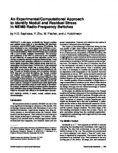
dure is subject to a dimensionality constraint, as well, which depends on the available computational capability and limits the admissible value of N1 and N2 . 3.1. The multi-level nesting algorithm. This section shows how to overcome the drawback on the size of N1 and N2 for the two-level nesting procedure by means of a multi-level nesting algorithm whose innermost procedure is represented by the simple nesting procedure of Corollary 3.1. The multi-level nesting algorithm reduces the computational effort needed to solve a finite-horizon LQ problem. The multi-level procedure basically corresponds to iteratively solving the second level N2 -step optimal control problem, stated in step 2, by means of a further nesting procedure. It is an easy matter to verify that the simple implementation of the iteration idea leads to increasing at each level the dimension of the matrices needed to compute the optimal cost keoN k22 . Property 1 enables overcoming the dimensionality drawback while iterating Algorithm 2 in the multi-level case. The multi-level nesting algorithm solves the N -step LQ optimal control problem as follows. Algorithm 3. step 1 Set k = 1 and Nk = N . step 2 Divide the control time interval in Nk = Nk,1 Nk,2 steps each, where Nk,1 is such that the computational complexity needed to evaluate the resolvent matrices TNk,1 , VNk,1 , CNk,1 and DNk,1 is met. Compute these matrices. ¯ N ∈ R(rk ×n) step 3 Compute the reduced-size cost matrices C¯Nk,1 ∈ R(rk ×n) and D k,1 as described in Property 1. step 4 State the second-level Nk,2 -step problem as defined in eq. (3.1), (3.3) and (3.4) with these reduced-size cost matrices. step 5 Solve the Nk,2 step problem if this is computationally possible. If not, set k = k + 1 and Nk = Nk,2 and go back to step 1. step 6 Move back over all the nested levels and assess the optimal control input and the cost for the original N -step problem. Table 3.1 illustrates a four-level nesting algorithm. At the second and third levels, k = 2 and k = 3, only basic matrices for the innermost problems are evaluated. The two-level nested problem is completely solved only at the last nesting level, i.e., k = 4. It is worth noting that if matrix factorization of Property 1 were not applied, the k k k k

=1 =2 =3 =4

N = N1,1 N1,2 N1 = N1,1 N1,2 = N2,1 N2,2 N1 = N2,1 N2,2 = N3,1 N3,2 N1 = N3,1 N2 = N3,2

Table 3.1 A four-level nested procedure. Matrices are evaluated only for problems with N1,1 , N2,1 , N3,1 and N3,2 steps.

dimensions of the matrices CNk,1 and DNk,1 would significantly increase with k. In Qk fact, at the nesting level k + 1 they would be both q j=1 Nj,1 × n , while factorization implies the maximum value rk+1 × n with rk+1 ≤ 2n at every step. 4. An example. As an illustrative example, let us consider the following constrained LQ optimal control problem for the system

9

A nested approach to the LQ control problem

3 0.5 1 −0.4 0 6 0.1 0.7 0 −0.5 7 7, A=6 4 0 0 0.4 0 5 0 0 0 0.6 2

3 1 0 6 0 1 7 7 B=6 4 1 0 5, 0 1 2

C=

1 0 0 0 0 1 0 0

,

D=

1 0 1 0.5

,

with initial condition x0 = [1, 2, 3, 4]0 , constrained final state and weighting matrix as 1 1

yf =

=

1 1 0 0 0 0 1 1

x(N ) ,

Z=

1 0 2 1 0 0 3 1

.

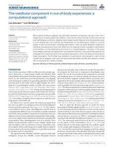
c 5.3 Problem 1 was first solved according to Algorithm 1 implemented in Matlab c

running on a 350 MhZ Pentium II. The corresponding CPU time was 77.72 s. Instead the CPU time corresponding to the implementation of Algorithm 2, with N1 = 25 and N2 = 8 was 0.676 s. Note that the three-levels nesting procedure, with N1,1 = 8, N2,1 = 5 and N2,2 = 5 yields a dramatic reduction of the CPU time: 0.16 s. results for CPU times are summarized in Table 4.1.

simple pseudoinversion N = 200 CPU time = 77.72 s two-level nesting N1 = 8; N2 = 25 CPU time = 0.676 s three-level nesting N1,1 = 8; N2,1 = 5; N2,2 = 5 CPU time = 0.16 s Table 4.1 CPU time is compared for different nesting level algorithms

It can be seen that the multi-level nesting algorithm greatly reduces the computational burden for the finite-horizon LQ optimal control problem. The optimal cost is min J = 0.687 , u200

and the final state 2

3 −0.4821 6 1.4821 7 7 x(200) = 6 4 −0.5109 5 . 1.5109

5. Concluding remarks. The problem considered in this paper is out of the standard scheme of the LQ optimal control problems considered in the literature, not only because of the completely general approach which makes it possible to deal with cheap, singular and regular problems with no distinction, but also because the state of the system can be sharply assigned at both the initial and final time instants. Furthermore, the proposed nesting procedure is very easily implementable thus making feasible the pseundoinversion solution of optimal control problems on a time interval of finite, but arbitrary, length. A practical application of the algorithms described herein are the computations of convolution profiles for H2 -optimal tracking and H2 -optimal rejection of an N -step previewed signal in the non-minimum phase case. These problems were described by the authors in [14, 15], where geometric-type conditions for perfect or almost perfect tracking or rejection with stability have been derived. The possibility of using the algorithmic setting described in this paper for the solution of the standard discrete-time infinite horizon LQR problem is under investigation.

10

G. MARRO, D. PRATTICHIZZO and E. ZATTONI

Acknowledgments. This work was partially supported by the Italian Ministry of University and Research.

A nested approach to the LQ control problem

11

Appendix. This appendix briefly presents the manipulations used in the proof of Theorem 2.1. Lemma 5.1. The problem of finding a vector λ which minimizes the 2-norm of the vector (5.1)

ζ := Φ λ + ρ¯ ,

and satisfies the constraint (5.2)

Γλ=σ ¯,

where the matrices Φ, Γ and the column vectors ρ¯ σ ¯ are given and the constraint (5.2) is assumed to be feasible (i.e., satisfying σ ¯ ∈ im Γ ), admits as the set of all solutions the linear variety (5.3)

#

#

λo (γ) := I − K (ΦK) Φ Γ # σ ¯ − K (ΦK) ρ¯ + P γ ,

where K is a basis matrix for ker Γ , P is a basis matrix for im K ∩ ker Φ and γ is a free vector parameterizing the solution λ in the column space of P . The corresponding ζ vector with minimum 2-norm is given by (5.4)

ζ o := I − ΦK (ΦK)

#

ΦΓ # σ ¯ + ρ¯ .

Proof. The constraint (5.2) can be solved with respect to λ as (5.5)

λ = Γ# σ ¯+Kν,

where ν parameterizes the solutions in ker Γ whose basis matrix is K. Then the following expression for vector ζ can be obtained by substituting eq. (5.5) in eq. (5.1) (5.6)

ζ = Ω ν + η¯ ,

where (5.7)

Ω := Φ K ,

η¯ := ΦΓ # σ ¯ + ρ¯ .

The expression for ν minimizing the 2-norm of ζ is simply obtained as (5.8)

ν = −Ω # η¯ + H γ ,

where vector γ parameterizes the solution in ker Ω whose basis matrix is H. The expression (5.9)

ζ o = I − Ω Ω # η¯

of the minimum norm vector ζ can then be obtained by substituting eq. (5.8) in eq. (5.6). Expression (5.4) for ζ o is derived from eq. (5.9) (5.7). By substituting eq. (5.8) in eq. (5.5), it follows that (5.10)

λ = Γ# σ ¯ − KΩ # η¯ + KH γ .

Moreover, since im H := ker (ΦK) = kerK + im Y ,

12

G. MARRO, D. PRATTICHIZZO and E. ZATTONI

with Y such that im (KY ) = im K ∩ ker Φ , eq. (5.10) can also be written as λ = Γ# σ ¯ − KΩ # η¯ + P γ ,

(5.11)

where P has been defined in the statement of the lemma. Finally, by substituting eq. (5.7) in eq. (5.11), linear variety (5.3) is obtained. Remark 5. The minimum 2-norm vector λ minimizing the cost function (5.1) is λo = I − P P #

I − K (ΦK)# Φ Γ # σ ¯ − K (ΦK)# ρ¯ ,

obtained by choosing γ = −P #

#

#

I − K (ΦK) Φ Γ # σ ¯ − K (ΦK) ρ¯ ,

eq. (5.3). If minimum norm is not required, a plainer expression for λ follows by assuming γ = 0. REFERENCES [1] B. Anderson and J. Moore, Optimal Control: Linear Quadratic Methods, Prentice Hall International, London, 1989. [2] W. Arnold and A. Laub, Generalized eigenproblem algorithms and software for algebraic Riccati equations, Proceedings of the IEEE, 72 (1984), pp. 1746–1754. [3] A. Bryson and Y. Ho, Applied Optimal Control, Blaisdell Publishing Company, Waltham, Massachussets, 1969. [4] B. Chen, H∞ control and its applications, vol. 235 of Lecture Notes in Control and Information Sciences, Springer-Verlag, New York, 1999. [5] T. Chen and B. Francis, Optimal Sampled-Data Control Systems, Springer, London, 1995. [6] T. Geerts, The algebraic Riccati equation and singular optimal control: the discrete-time case, in Proceedings of the International Symposium on Systems and Networks: Mathematical Theory and Applications (MTNS ’93), vol. 2, Regensburg, Germany, August 2–6, 1993, pp. 129–134. [7] G. Golub and C. Van Loan, Matrix Computations, The Johns Hopkins University Press, Baltimore, MD, 2nd ed., 1989. [8] M. Hautus and L. Silverman, System structure and singular control, Linear Algebra and Its Applications, 50 (1983), pp. 369–402. ˘ and M. Weiss, General matrix pencil techniques for the solution of [9] C. Ionescu, V. Oara algebraic Riccati equation: a unified approach, IEEE Transactions on Automatic Control, 42 (1997), pp. 1085–1097. ˘, Generalized continuous-time Riccati theory, Linear Algebra and Its [10] V. Ionescu and C. Oara Applications, 232 (1996), pp. 111–130. [11] V. Ionescu and M. Weiss, On computing the stabilizing solution of the discrete-time Riccati equation, Linear Algebra and Its Applications, 174 (1992), pp. 229–238. [12] H. Kwakernaak and R. Sivan, Linear Optimal Control Systems, John Wiley & Sons, New York, 1972. [13] F. Lewis and V. Syrmos, Optimal Control, John Wiley & Sons, New York, 1995. [14] G. Marro, D. Prattichizzo, and E. Zattoni, Convolution profiles for noncausal inversion of multivariable discrete-time systems, in Proceedings of the 8th IEEE Mediterranean Conference on Control & Automation (MED 2000), P. Groumpos, N. Koussoulas, and P. Antsaklis, eds., University of Patras, Rio, Greece, July 17th–19th, 2000. , A unified algorithmic setting for signal-decoupling compensators and unknown input [15] observers, in Proceedings of the 39th IEEE Conference on Decision and Control (CDC 2000), Sydney, Australia, December 12–15, 2000.

A nested approach to the LQ control problem

13

[16] A. Ran and H. Trentelman, Linear quadratic problems with indefinite cost for discrete time, SIAM J. Matrix Anal. Appl., 14 (1993), pp. 776–797. [17] A. Saberi and P. Sannuti, Cheap and singular controls for linear quadratic regulators, IEEE Transactions on Automatic Control, AC-32 (1987), pp. 208–219. [18] A. Saberi, P. Sannuti, and B. Chen, H2 Optimal Control, System and Control Engineering, Prentice Hall International, London, 1995. [19] L. Silverman, Inversion of multivariable linear systems, IEEE Transactions on Automatic Control, AC-14 (1969), pp. 270–276. [20] L. Silverman, Discrete Riccati equations: alternative algorithms, asymptotic properties, and system theory interpretations, in Control and Dynamic Systems, C. Leondes, ed., Academic Press, New York, 1976, pp. 313–386. [21] J. Soethoudt and H. Trentelman, The regular indefinite linear-quadratic problem with linear endpoint constraints, Systems and Control Letters, 12 (1989), pp. 23–31. [22] A. Stoorvogel and A. Saberi, The discrete-time algebraic Riccati equation and linear matrix inequality, Linear Algebra and its Applications, 274 (1998), pp. 317–365. [23] P. Van Dooren, A generalized eigenvalue approach for solving the Riccati equation, SIAM J. Sci. Stat. Comp., 2 (1981), pp. 121–135.