COMPUTATIONAL MODEL OF THE MARK-IV ELECTROREFINER ...

COMPUTATIONAL MODEL OF THE MARK-IV ELECTROREFINER: TWO-DIMENSIONAL POTENTIAL AND CURRENT DISTRIBUTIONS

PYROMETALLURGICAL REPROCESSING KEYWORDS: electrochemical processing, electrorefiner, potential distribution

ROBERT O. HOOVER,a * SUPATHORN PHONGIKAROON,a MICHAEL F. SIMPSON,b TAE-SIC YOO,b and SHELLY X. LI b a

University of Idaho-Idaho Falls, Center for Advanced Energy Studies Department of Chemical Engineering, Nuclear Engineering Program 995 University Boulevard, Idaho Falls, Idaho 83402 b Idaho National Laboratory, Pyroprocessing Technology Department P.O. Box 1625, Idaho Falls, Idaho 83415

Received January 10, 2010 Accepted for Publication May 17, 2010

A computational model of the Mark-IV electrorefiner is currently being developed as a joint project between Idaho National Laboratory, Korea Atomic Energy Research Institute, Seoul National University, and the University of Idaho. As part of this model, the two-dimensional potential and current distributions within the molten salt electrolyte are calculated for U 3⫹, Zr 4⫹, and Pu 3⫹ along with the total distributions, using the partial differential equation solver of the commercial Matlab software. The electrical conductivity of the electrolyte solution is shown to depend primarily on the composition of the electrolyte

and to average 205 mho/m with a standard deviation of 2.5 ⫻ 10⫺5 % throughout the electrorefining process. These distributions show that the highest potential gradients (thus, the highest current) exist directly between the two anodes and cathode. The total, uranium, and plutonium potential gradients are shown to increase throughout the process, with a slight decrease in that of zirconium. The distributions also show small potential gradients and very little current flow in the region far from the operating electrodes.

I. INTRODUCTION

as direct disposal because of the highly exothermic reaction between sodium and water. To overcome this issue, Argonne National Laboratory ~ANL! developed an electrochemical process for treating the inventory of sodium-bonded spent fuel, at the center of which lies the Mark-IV electrorefiner.2 The process begins with spent fuel rods being chopped into short, 0.25-in. ~0.635-cm! segments, which are then loaded into stainless steel fuel dissolution baskets ~FDBs!. Four of these FDBs are combined into a cruciform shape, which forms an anode within the electrorefiner.3 A power source is used to apply a potential across the electrodes, causing the oxidation of uranium and the more active species in the spent fuel, which then dissolve into a LiCl-KCl eutectic molten salt. Simultaneously, essentially pure uranium is reduced back to metal and deposited onto a solid steel cathode, resulting in the reactions as described by

The Experimental Breeder Reactor–II ~EBR-II! is a sodium-cooled fast reactor that was operated at Argonne National Laboratory–West, now Idaho National Laboratory ~INL!, from 1963 through 1994 ~Ref. 1!. This reactor operated on a highly enriched uranium–10% zirconium alloy as driver fuel surrounded by a blanket of depleted uranium fuel for plutonium breeding. During its 30⫹ years of operation, large amounts of both spent driver and blanket fuel have accumulated. This metallic fuel contains sodium metal as a thermal bond between the fuel pins and stainless steel cladding, which has alloyed with the fuel. This metallic sodium creates issues with both conventional aqueous processing techniques as well *E-mail: [email protected] 176

NUCLEAR TECHNOLOGY

VOL. 173

FEB. 2011

Hoover et al.

COMPUTATIONAL MODEL OF THE MARK-IV ELECTROREFINER

Eqs. ~1a!, ~1b!, and ~1c!. This uranium contains salt, which is removed by distillation, leaving a uranium product ingot for eventual disposal. Anode: Mi ~anode! r Min⫹ ~salt ! ⫹ ni e ⫺ ,

~1a!

Cathode: Min⫹ ~salt ! ⫹ ni e ⫺ r Mi ~cathode! ,

~1b!

determination of where within the electrorefiner the ions of the different species are moving and where they are essentially motionless. The total ohmic resistance of the electrolyte is highly dependent on the potential and current distributions as well. Decreasing this resistance is an essential matter in increasing the electrical efficiency of the system.

and Net reaction: Mi ~anode! r Mi ~cathode! .

~1c!

Following electrorefining, the cladding and noble metals, including zirconium, that remain in the FDBs are blended with more zirconium to create a metal waste form. Over time, fission products build up in the molten salt, which is periodically processed into a ceramic waste form.4 To better understand the processes occurring within the Mark-IV electrorefiner, computational models have been developed by ANL ~Refs. 5, 6, and 7!, Iizuka et al.8 in Japan, and Nawada et al.9 and Nawada and Bhat 10 in India. Ahluwalia et al.5 and Ahluwalia and Hua 6 at ANL developed an advanced intensive computational model to help in understanding the different possible modes of electrorefining ~i.e., direct transport, deposition, anodic dissolution, cathode stripping, and drawdown!. Vaden,7 also at ANL, developed a chemical equilibrium model dealing with purely chemical reactions occurring among the molten salt and the FDBs and the cadmium pool. The model presented by Iizuka et al.8 deals only with anodic dissolution, and the model described by Nawada et al.9 and Nawada and Bhat 10 examines transport from a liquid cadmium anode. Currently, a computational model is being developed as a joint project between INL, Korea Atomic Energy Research Institute ~KAERI!, Seoul National University ~SNU!, and the University of Idaho ~UI!. KAERI and SNU have been developing a rigorous three-dimensional ~3-D! model,11 and INL and UI have been focusing on a less computationally intensive two-dimensional ~2-D! model.12,13 These two computational models are being developed based on fundamental electrochemical, thermodynamic, and kinetic theories. The models will be used to cross-evaluate each other and compare the utility of a rigorous 3-D model with a simpler 2-D model. The model being developed by INL and UI will be an invaluable tool for optimizing operating parameters and determining their effect on the electrochemical process outputs. The model will also aid in determining how used nuclear fuel from different types of reactors, containing different fuel constituents, will act within the electrorefiner. As an integral part of the development of this computational model, the 2-D potential and current distributions have been calculated for U 3⫹, Zr 4⫹, and Pu 3⫹—these three species collectively constitute .90 wt% of the EBR-II spent driver fuel.3 These distributions are essential in determining the mass balance and location of the different species throughout the electrorefiner. The current distribution allows the NUCLEAR TECHNOLOGY

VOL. 173

FEB. 2011

II. MODEL DEVELOPMENT A material balance of the Mark-IV electrorefiner can be performed, resulting in 14 ]ci ]t

⫽ ⫺¹{Ni ,

~2!

where ci ⫽ concentration of species i t ⫽ time Ni ⫽ molar flux of species i. Multiplying Eq. ~2! by the valence number z i of species i and Faraday’s constant F and summing over all species yields ] ]t

F ( z i ci ⫽ ⫺¹{F ( z i Ni . i

~3!

i

The current through the bulk electrolyte is carried by the motion of all the ions in the solution, which can be expressed as i ⫽ F ( z i Ni ,

~4!

i

where i is the total current density. It is also known that the bulk electrolyte must remain electrically neutral, and therefore the electroneutrality condition ~ (i z i ci ⫽ 0! holds. Using Eq. ~4! and the electroneutrality condition, Eq. ~3! simplifies to ¹{i ⫽ 0 .

~5!

The flux of a species under both a potential and concentration gradient can be described by Ni ⫽ ⫺z i u i Fci ¹f ⫺ Di ¹ci ⫹ ci v ,

~6!

where u i ⫽ ionic mobility f ⫽ potential Di ⫽ diffusion coefficient v ⫽ bulk fluid velocity. 177

Hoover et al.

COMPUTATIONAL MODEL OF THE MARK-IV ELECTROREFINER

Substituting this into Eq. ~4! yields i ⫽ ⫺F 2 ¹f ( z i2 u i ci ⫺ F ( z i Di ¹ci ⫹ Fv ( z i ci . i

i

i

~7! Assuming the bulk electrolyte is well mixed, which implies that there are no concentration gradients within the bulk, and applying the electroneutrality condition, the second and third terms of Eq. ~7! become zero. The simplified version of Eq. ~7! becomes i ⫽ ⫺F 2 ¹f ( z i2 u i ci .

~8!

i

With the definition of conductivity,14 k ⫽ F 2 ( z i2 u i ci ,

~9!

i

Eq. ~8! is even further simplified into a version of Ohm’s law, i ⫽ ⫺k¹f .

~10!

Plugging this expression into Eq. ~5! and assuming uniform temperature and concentration within the bulk, Laplace’s equation is found to describe the potential distribution 14 : ¹2f ⫽ 0 .

~11!

The Laplace equation is solved in order to find the potential distribution. From the solution and Eq. ~10!, the current distribution is solved. III. COMPUTATIONAL PROCEDURES The commercial software Matlab has previously been used by the authors in the development of the Mark-IV computational model.12,13 This software contains a partial differential equation ~PDE! solver using the finite element method, which is used to calculate the potential distribution within the electrolyte. The PDE solver is embedded into the model, receiving inputs calculated from the model. The first step in calculating the potential distribution is setting up the geometry of the electrorefiner itself. Thorough descriptions of this geometry by Li and Simpson,3 Li et al.,15 and Kim et al.11 have been published previously. Data from a specific experimental run in the Mark-IV electrorefiner have been obtained from Ref. 3 to aid in the development of the computational model. In this run, the electrorefiner was operated at 5008C with two anodes and one solid steel cathode, as shown in Fig. 1. The geometry was set up in Cartesian coordinates with the origin at the center of the electrorefiner, as shown in Fig. 1. The voltage is applied between the anodes and cathode so that the two anodes are at the same potential. 178

Fig. 1. Geometry of the Mark-IV electrorefiner.

Both anodes and the cathode were rotated at 5 rpm, and for simplicity, the spinning cruciform anodes and dendritically growing cathode are considered cylindrical. The radius of the cathode increases throughout the electrorefining process as a function of the amount of deposited uranium, or more accurately, the total coulombs. The outer shell of the electrorefiner, the baffles, and the central stir rod can be assumed to be electrically insulated from the electrolyte, and therefore a Neumann boundary condition, ¹f ⫽ 0, is applied at these boundaries. The boundary conditions at the cathode and anode surfaces are slightly more complicated, as depicted in Fig. 2. The partial potentials with respect to a Ag0AgCl reference electrode in the electrolyte at the anodes and cathode are DEi, a and DEi, c , respectively, and these are

Fig. 2. Electrolytic cell potential diagram ~DEt, c and DEt, a are total cathode and anode potentials, DEi, c and DEi, a are partial cathode and anode potentials of species i, hi, c and hi,a are surface overpotentials of species i, and Dfohm is the ohmic potential drop through the electrolyte!. NUCLEAR TECHNOLOGY

VOL. 173

FEB. 2011

Hoover et al.

COMPUTATIONAL MODEL OF THE MARK-IV ELECTROREFINER

used as the boundary conditions at these locations for each individual species’ potential distribution, as shown in Fig. 3. For the total potential distribution, the total anode and cathode potentials are used as the boundary condition. The computational model calculates these values ~along with many others, including current and overpotentials! and outputs them to the PDE solver. With the given parameters for the specific experimental run, the partial potentials versus a Ag0AgCl reference electrode as calculated by the model are shown throughout the experiment in Fig. 4. There is little plutonium ~,0.4 wt%! present in the spent driver fuel, which is rapidly ~,20 min! oxidized from the anode. Therefore, throughout the majority of the electrorefining process, no plutonium reaction is occurring and the partial potentials of plutonium are the same as the total electrode potentials. The difference between partial and total potential at either electrode is related to the rate at which the species is either oxidized or reduced. As can be seen in Fig. 4, the reactions of uranium occur at greater rates than the other species. However, as the electrorefining process proceeds, more zirconium is being both dissolved from the anode and deposited at the cathode. The potential differences occur because of several influential factors such as differing dissolution and deposition rates, increasing resistance to mass transfer, and decreasing surface area. These factors have been reported and discussed in detail by Hoover et al.13 Throughout the majority of the electrorefining process, the partial potentials of plutonium are the same as the total potential. Here, DEt and DEU increase slightly, whereas DEZr decreases. This trend occurs because as the process proceeds and the amount of uranium available to be dissolved at the anode decreases, a greater potential is necessary to support the same current. This higher total

Fig. 4. Anode and cathode boundary conditions during the modeled electrochemical process.

potential allows more zirconium to be dissolved, increasing its overpotential and decreasing its potential difference. This shows that in order to minimize zirconium dissolution and maximize the purity of the uranium collected at the cathode, the total uranium dissolution must be limited. Unfortunately, one of the main goals of the electrochemical process is to maximize uranium collection while minimizing that of zirconium.3 Following the input of boundary conditions, the triangular mesh is created, with edge lengths ranging from 0.2 to 4 cm, with tighter meshing surrounding the stir rod and baffles and between the cathode and cathode scraper. Following the described setup, the PDE solver within Matlab is used to numerically solve the Laplace Eq. ~11!, in two-dimensional Cartesian coordinates: ] 2f ]x 2

⫹

] 2f ]y 2

⫽0 .

~12!

IV. RESULTS AND DISCUSSION From the solution to the potential distribution, the current distribution is calculated using Eq. ~10!. To accomplish this, the electrical conductivity k of the bulk electrolyte needs to be calculated. For the modeled system containing Li⫹, K⫹, U 3⫹, Zr 4⫹, Pu 3⫹, and Cl⫺ ions, the conductivity can be calculated as 2 2 k ⫽ F 2 ~z Li u Li cLi ⫹ z K2 u K cK ⫹ z U2 u U cU ⫹ z Zr uZrcZr 2 2 ⫹ zPu u Pu cPu ⫹ z Cl u Cl cCl ! .

Fig. 3. Boundary conditions for the solution of the potential distribution. NUCLEAR TECHNOLOGY

VOL. 173

FEB. 2011

~13!

Assuming a dilute system, ionic mobility u i can be calculated from the diffusion coefficient Di ~Ref. 14!: 179

Hoover et al.

COMPUTATIONAL MODEL OF THE MARK-IV ELECTROREFINER

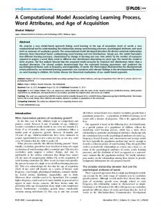
Fig. 6. Total current distribution at ~a! 10, ~b! 40, and ~c! 70 h into the experimental run.

Fig. 5. Total potential distribution at ~a! 10, ~b! 40, and ~c! 70 h into the experimental run.

Di ⫽ RTu i .

~14!

Diffusion coefficients, calculated ionic mobilities, and average bulk concentrations for all six ions present in the electrolyte at 5008C are listed in Table I. 180

From this information, the average conductivity of the bulk electrolyte solution is calculated to be 205 mho0m with a standard deviation of 2.5 ⫻ 10⫺5 % due to the change in species composition throughout the electrorefining process. Using this method, the conductivity of the pure LiCl0KCl eutectic is calculated to be 188 mho0m. This value compares well with the experimental value of 187.223 mho0m reported by Van Artsdalen and Yaffe.18 The solutions to the total potential distribution at 10, 40, and 70 h into the experiment are plotted in Fig. 5. The current distributions at these times are shown in Fig. 6. NUCLEAR TECHNOLOGY

VOL. 173

FEB. 2011

Hoover et al.

COMPUTATIONAL MODEL OF THE MARK-IV ELECTROREFINER

TABLE I Diffusion Coefficients, Ionic Mobilities, and Average Concentrations Di ~m 20s! U 3⫹ Zr 4⫹ Pu 3⫹ Li⫹ K⫹ Cl⫺

1.45 ⫻ 10⫺9 1.13 ⫻ 10⫺9 1.08 ⫻ 10⫺9 1.9 ⫻ 10⫺9 2.4 ⫻ 10⫺9 2.5 ⫻ 10⫺9

~Ref. 16! ~Ref. 16! ~Ref. 16! ~Ref. 17! ~Ref. 17! ~Ref. 17!

The partial potential and current distributions look essentially the same, with differences only in the absolute values. It is clear from both the potential and current distributions that the majority of the current flows directly between the two anodes to the cathode. The current distribution shows this characteristic, and the potential distribution shows that this is the area of steepest potential gradient. The potential distribution can be thought of as a topographical map with the lighter ~higher-potential! regions being the high elevations and the darker ~lower-potential! regions being the lower elevations. The current can be thought of as many balls rolling from the high mountains at the anodes to the low valley at the cathode. All these balls spread out, yet they tend to roll down the steepest paths toward the valley. Likewise, the current tends to flow from the high-potential to the low-potential regions through the areas with higher-potential gradients. Nevertheless, it is important to note that substantial energy is required to transfer the balls back to the mountaintops. This energy is in the form of system heating and applied potential across the electrodes in an electrochemical cell such as the Mark-IV electrorefiner. At all times the potential varies from higher values ~less negative! at the anodes to lower values ~more negative! surrounding the cathode. The potential gradient between the electrodes increases throughout the process up to ;39 h, when the cathode is removed and replaced with a fresh one. This is why the cathode at 40 h in Figs. 5b and 6b is smaller than those at 10 and 70 h in Figs. 5a, 5c, 6a, and 6c. The potential gradient in the lower regions of Figs. 5 and 6 is small, with very little current and therefore few moving ions, throughout the modeled experiment. Hence, a possible second cathode could be placed in this region to better use the available space within the electrorefiner.

ui ~m 2 {mol0J{s!

ci ~mol0m 3 !

2.26 ⫻ 10⫺13 1.76 ⫻ 10⫺13 1.68 ⫻ 10⫺13 3.0 ⫻ 10⫺13 3.8 ⫻ 10⫺13 3.9 ⫻ 10⫺13

560 6 0.06 0.106 6 0.04 18.1 6 0.007 16 500 6 2 ⫻ 10⫺10 11 500 6 2.5 ⫻ 10⫺10 29 700 6 1.5 ⫻ 10⫺4

been examined. Different species such as U 3⫹, Zr 4⫹, and Pu 3⫹ can currently be calculated and evaluated using this technique. The electrical conductivity of the molten salt electrolyte depends on composition and is shown to be 205 mho0m throughout the electrorefining process. The potential distribution shows that the highest potential gradients exist directly between the anodes and cathode. In general, the uranium, plutonium, and total potential gradients increase throughout the process, whereas the zirconium potential gradients decrease. The result shows that as the electrorefining progresses, more zirconium and less uranium and plutonium are being electrotransported. The regions farthest from the operating electrodes have small potential gradients and little ion movement. From this observation, to take full advantage of the electrorefiner’s geometry, it is recommended that these regions be utilized by adding an additional cathode.

ACKNOWLEDGMENTS This research was supported financially by the U.S. Department of Energy under the Fuel Cycle Research and Development program. It was carried out within the U.S.0Republic of Korea International Nuclear Energy Research Initiative ~I-NERI! program ~project 2007-006-K!.

REFERENCES 1. S. M. STACY, Proving the Principle: A History of the Idaho National Engineering and Environmental Laboratory, 1949–1999, p. 137, Idaho Operations Office of the Department of Energy, Idaho Falls, Idaho ~2000!. 2. R. K. AHLUWALIA and T. Q. HUA, U.S. Patent 6,689,260 ~Feb. 10, 2004!.

V. SUMMARY The 2-D potential and current distributions within the bulk electrolyte of the Mark-IV electrorefiner have NUCLEAR TECHNOLOGY

VOL. 173

FEB. 2011

3. S. X. LI and M. F. SIMPSON, “Anodic Process of Electrorefining Spent Driver Fuel in Molten LiCl-KCl-UCl30Cd System,” J. Mineral Metallurg. Process., 22, 192 ~2005!. 181

Hoover et al.

COMPUTATIONAL MODEL OF THE MARK-IV ELECTROREFINER

4. B. R. WESTPHAL and R. D. MARIANI, “Uranium Processing During the Treatment of Sodium-Bonded Spent Nuclear Fuel,” J. Minerals, Metals, Mater. Soc., 52, 21 ~2000!. 5. R. AHLUWALIA, T. Q. HUA, and H. K. GEYER, “Behavior of Uranium and Zirconium in Direct Transport Tests with Irradiated EBR-II Fuel,” Nucl. Technol., 126, 289 ~1999!. 6. R. K. AHLUWALIA and T. Q. HUA, “Electrotransport of Uranium from a Liquid Cadmium Anode to a Solid Cathode,” Nucl. Technol., 140, 41 ~2002!.

12. R. O. HOOVER, S. PHONGIKAROON, S. X. LI, M. F. SIMPSON, and T. YOO, “A Computational Model of the Mark-IV Electrorefiner: Phase I—Fuel Basket0Salt Interface,” J. Eng. Gas Turbines Power, 131, 054503-1– 4 ~2009!. 13. R. O. HOOVER, S. PHONGIKAROON, M. F. SIMPSON, S. X. LI, and T.-S. YOO, “Development of Computational Models for the Mark-IV Electrorefiner—Effect of Uranium, Plutonium, and Zirconium Dissolution at the Fuel Basket–Salt Interface,” Nucl. Technol., 171, 276 ~2010!.

7. D. VADEN, “Fuel Conditioning Facility Electrorefiner Process Model,” Sep. Sci. Technol., 41, 2003 ~2006!.

14. G. PRENTICE, Electrochemical Engineering Principles, p. 165, Prentice Hall, Upper Saddle River, New Jersey ~1991!.

8. M. IIZUKA, K. KINOSHITA, and T. KOYAMA, “Modeling of Anodic Dissolution of U-Pu-Zr Ternary Alloy in the Molten LiCl-KCl Electrolyte,” J. Phys. Chem. Solids, 66, 427 ~2005!.

15. S. X. LI, T. SOFU, T. A. JOHNSON, and D. V. LAUG, “Experimental Observations on Electrorefining Spent Nuclear Fuel in Molten LiCl-KCl0Liquid Cadmium System,” J. New Mater. Electrochem. Syst., 3, 259 ~2000!.

9. H. P. NAWADA, N. P. BHAT, and G. R. BALASUBRAMANIAN, “Development of a Computer Code for Modeling Electrorefining Process for Reprocessing Spent Metallic Fuel,” Bull. Electrochem., 12, 333 ~1996!.

16. D. YAMADA, T. MURAI, K. MORITANI, T. SASAKI, I. TAKAGI, H. MORIYAMA, K. KINOSHITA, and H. YAMANA, “Diffusion Behavior of Actinide and Lanthanide Elements in Molten Salt for Reductive Extraction,” J. Alloys Compounds, 444–445, 557 ~2007!.

10. H. P. NAWADA and N. P. BHAT, “Thermochemical Modelling of Electrotransport of Uranium and Plutonium in an Electrorefiner,” Nucl. Eng. Des., 179, 75 ~1998!. 11. K. R. KIM, S. Y. CHOI, D. H. AHN, S. PAEK, B. G. PARK, H. S. LEE, K. W. YI, and I. S. HWANG, “Computational Analysis of a Molten-Salt Electrochemical System for Nuclear Waste Treatment,” J. Radioanalyt. Nucl. Chem. ~July 10, 2009!.

182

17. C. CACCAMO and M. DIXON, “Molten Alkali-Halide Mixtures: A Molecular-Dynamics Study of Li-KCl Mixtures,” J. Phys. C: Solid State Phys., 13, 1887 ~1980!. 18. E. R. VAN ARTSDALEN and I. S. YAFFE, “Electrical Conductance and Density of Molten Salt Systems: KCl-LiCl, KCl-NaCl and KCl-KI,” J. Phys. Chem., 59, 118 ~1955!.

NUCLEAR TECHNOLOGY

VOL. 173

FEB. 2011