access (NAMA), the link activation multiple access (LAMA) and pair-wise link activation multiple access (PAMA). In addition, HAMA achieves better throughout ...
Computational Time-Division and Code-Division Channel Access Scheduling in Ad Hoc Networks Lichun Bao and J.J. Garcia-Luna-Aceves
Abstract— Using two-hop neighborhood information, we present the hybrid activation multiple access (HAMA) protocol for time-division channel access scheduling in ad hoc networks with omni-directional antennas. Different from other approaches, HAMA is a node-activation channel access protocol that also maximizes the chance of link activations using time- and code-division schemes. The throughput and delay characteristics of HAMA in randomly-generated multihop wireless networks are studied by analyses and simulations. The results of the analyses show that HAMA achieves higher channel utilization in ad hoc networks than previous similar works, namely, the node activation multiple access (NAMA), the link activation multiple access (LAMA) and pair-wise link activation multiple access (PAMA). In addition, HAMA achieves better throughout than an existing scheduling algorithm based on complete topology information, and much higher throughout than the ideal CSMA and CSMA/CA protocols. The main contribution of this work is to computationally derive channel access schedules according to local network topology information instead of on-demand negotiations or static global coordinations. Index Terms— Channel access scheduling, medium access control protocol, MAC, ad hoc networks.
I. I NTRODUCTION Channel access protocols for ad hoc networks can be non-deterministic or deterministic. The non-deterministic scheme includes approaches such as ALOHA, CSMA [1] and several collision avoidance mechanisms in the IEEE 801.11 standards [2]. However, as the network load increases, network throughput drastically degrades because the probability of collisions rises, preventing stations from acquiring the channel. The deterministic access schemes set up timetables for individual nodes or links, such that the transmissions from the nodes or over the links are conflict-free in the code, time, frequency or space divisions of the channel. The schedules for conflict-free channel access can be established based on the topology of the network, or it can be topology independent. Topology-dependent channel access control algorithms can establish transmission schedules by either dynamically exchanging and resolving time slot requests [3]– [5], or pre-arrange a time-table for each node based on the network topologies. Setting up a conflict-free channel access time-table is typically treated as a node- or linkcoloring problem on graphs representing the network topologies. The problem of optimally scheduling access to a common channel is one of the classic NP-hard problems in graph theory (k-colorability on nodes or edges) [6]–[8]. Polynomial algorithms are known to achieve suboptimal solutions using randomized approaches or heuristics based on such graph attributes as the degree of the nodes.
A unified framework for TDMA/FDMA/CDMA channel assignments, called UxDMA algorithm, was described by Ramanathan [9]. UxDMA summarizes the patterns of many other channel access scheduling algorithms in a single framework. These algorithms are represented by UxDMA with different parameters. The parameters in UxDMA are the constraints put on the graph entities (nodes or links) such that entities related by the constraints are colored differently. Based on the global topology, UxDMA computes the node or edge coloring, which correspond to channel assignments to these nodes or links in the time, frequency or code domain. A number of topology-transparent scheduling methods have been proposed to provide conflict-free channel access that is independent of the radio connectivity around any given node [10]–[12]. The basic idea of the topologytransparent scheduling approach is for a node to transmit in a number of time slots in each time frame. The times when node i transmits in a frame corresponds to a unique code such that, for any given neighbor k of i, node i has at least one transmission slot during which node k and none of k’s own neighbors are transmitting. Therefore, within any given time frame, any neighbor of node i can receive at least one packet from node i conflict-free. An enhanced topology-transparent scheduling protocol, TSMA (Time Spread Multiple Access), was proposed by Krishnan and Sterbenz [12] to reliably transmit control messages with acknowledgments. However, TSMA performs worse than CSMA in terms of delay and throughput [12]. We propose a neighbor-aware contention resolution (NCR) algorithm. Using only the identifiers of the contenders and the current contention context number, NCR computes a randomized priority for each contender in a given contention context. Then, each contender locally determines its eligibility to access the resource in the contention context by comparing its priority with other contenders’. Because the scheduling is dynamic, depending on the contention contexts, a different schedule is established in each contention context. The main contribution of this approach is to computationally derive channel access schedules according to local network topology information instead of on-demand negotiations or static global coordinations as chosen by the previous methods. Based on NCR, we design a new hybrid activation multiple access protocol (HAMA), which supports broadcast, multicast and unicast communications through code- and time-division multiple access in wireless networks. The difference with the node-activation and link-activation protocols proposed in [13] is that HAMA schedules
the channel access for broadcast while maximizing the chances of unicast at the same time, whereas the previous protocols are capable of supporting only node- or linkactivation, but not both. The rest of the paper is organized as follows. Section II presents the NCR algorithm and analyzes the packet delay encountered in a general queuing model under certain contention level. Section III describes HAMA. Section IV derives the channel access probabilities of HAMA in uniformly distributed ad hoc networks, and compares the throughput attributes of HAMA with those of other channel access scheduling approaches as well as idealized CSMA and CSMA/CA schemes. Section V presents the results of simulations that provide further insights on the performance differences among the various scheduling protocols. II. N EIGHBOR -AWARE C ONTENTION R ESOLUTION (NCR) S PECIFICATION No limited to ad hoc network scenarios, the neighboraware contention resolution (NCR) envisions a special election problem for an entity to locally decide the leadership status of itself among a known set of contenders in any given contention context. We assume that the knowledge of the contenders for each entity is acquired by an appropriate means, depending on the specific applications. For example, in the ad hoc networks of our interest, the contenders of each node are the neighbors within two hops, which can be obtained by each node periodically broadcasting the identifiers of its one-hop neighbors [14]. Furthermore, NCR requires that each contention context be identifiable, such as the time slot number in networks based on a time-division multiple access scheme. Thus, the election problem for neighbor-aware contention resolution is be formulated as :“Given a set of contenders, Mi , against entity i in contention context t, how should the precedence of entity i in the set Mi ∪ {i} be established, such that every other contender yields to entity i whenever entity i establishes itself as the leader for the shared resource?” To decide the precedence of an entity without incurring communication overhead among the contenders, we assign the entity a priority that depends on the identifier of the entity and varies according to the known contention context so that the criterion for the leadership is deterministic and fair among the contenders. Eq. (1) provides a formula to derive the priority, denoted by i.prio, for entity i in contention context t. i.prio = Hash(i ⊕ t) ⊕ i,
(1)
where the function Hash(x) is a fast message digest generator that returns a random integer in range [0, M ] by hashing the input value x, and the sign ‘⊕’ is designated to carry out the concatenation operation on its two operands. Note that, while the Hash function can generate the same number on different inputs, each priority number is unique because the priority is appended with identifier of the entity.
NCR(i, t) { /* Initialize. */ 1 for (k ∈ Mi ∪ {i}) 2 k.prio = Hash(k ⊕ t) ⊕k; /* Resolve leadership. */ 3 if (∀k ∈ Mi , i.prio > k.prio) 4 i is the leader; } /* End of NCR. */ Figure 1. NCR Specification.
Figure 1 describes the NCR algorithm. Basically, NCR generates a permutation of the contending members, the order of which is decided by the priorities of all participants. Because it is assumed that contenders have mutual knowledge and t is synchronized, the order of contenders based on the priority numbers is consistent at every participant, thus avoiding any conflict among contenders. III. H YBRID ACTIVATION M ULTIPLE ACCESS (HAMA) A. Modeling of Network and Contention We assume that each node is assigned a unique identifier, and is mounted with an omni-directional radio transceiver that is capable of communicating using DSSS (direct sequence spread spectrum) on a pool of wellchosen spreading codes. The radio of each node only works in half-duplex mode, i.e., either transmit or receive data packet at a time, but not both. In multihop wireless networks, signal collisions may be avoided if the received radio signals are spread over different codes or scattered onto different frequency bands. Because the same codes on certain different frequency bands can be equivalently considered to be on different codes, we only consider channel access based on a code division multiple access scheme. Time is synchronized at each node, and nodes access the channel based on slotted time boundaries. Each time slot is long enough to transmit a complete data packet, and is numbered relative to a consensus starting point. Although global time synchronization is desirable, only limited-scope synchronization is necessary for scheduling conflict-free channel access in multihop ad hoc networks, as long as the consecutive transmissions in any part of the network do not overlap across time slot boundaries. Time synchronization is outside the scope of this paper. The topology of a packet radio network is represented by an undirected graph G = (V, E), where V is the set of network nodes, and E is the set of links between nodes. The existence of a link (u, v) ∈ E implies that (v, u) ∈ E, and that node u and v are within the transmission range of each other, so that they can exchange packets via the wireless channel. In this case, u and v are called one-hop neighbors of each other. The set of one-hop neighbors of a node i is denoted by Ni1 . Two nodes are called twohop neighbors of each other if they are not adjacent, but have at least one common one-hop neighbor. The neighbor
information of node i refers to the union of the one-hop neighbors of i itself and the one-hop neighbors of i’s onehop neighbors, which equals [ Ni1 ∪ ( Nj1 ) . j∈Ni1
To ensure conflict-free transmissions, it is sufficient for nodes within two hops to not transmit on the same time, code and frequency coordinates [16]. Therefore, a node should at least know the topology information within two hops for conflict-free channel access scheduling. The operation of HAMA assumes that each node already knows its neighbor information within two hops. B. Code Assignment HAMA is a time-slotted code division multiple access scheme based on direct sequence spread spectrum (DSSS) transmission techniques. In DSSS, code assignments are categorized into transmitter-oriented, receiver-oriented or a per-link-oriented code assignment schemes (also known as TOCA, ROCA and POCA, respectively) in ad hoc networks (e.g. [17] [18]). HAMA adopts transmitter-oriented code assignment because of its broadcast capability. We assume that a pool of well-chosen orthogonal pseudo-noise codes, Cpn = {ck | k = 0, 1, · · ·}, is available in the signal spreading function. During each time slot t, a spreading code is assigned to node i, denoted by i.TxCode, as given by Eq. (2). i.TxCode = ck , k = Hash(i ⊕ t) mod |Cpn | .
(2)
Hash(x) is a fast message digest generator that returns a random integer by hashing the input value x. The sign ‘⊕’ is designated to carry out the concatenation operation on its two operands. Unlike previous channel access scheduling protocols that activate either nodes or links only, HAMA (hybrid activation multiple access) is a node-activation channel access protocol that is capable of broadcast transmissions, while also maximizing the chance of link activations for unicast transmissions. The code assignment in HAMA is the TOCA scheme. In each time slot, a node derives its state by comparing its own priority with the priorities of its neighbors. We require that only nodes with higher priorities transmit to those with lower priorities. Accordingly, HAMA defines the following node states: R Receiver: The node has an intermediate priority among its one-hop neighbors. D Drain: The node has the lowest priority among its one-hop neighbors, and can only receive a packet in the time slot. BT Broadcast Transmitter: the node has the highest priority within its two-hop neighborhood, and can broadcast to its one-hop neighbors. UT Unicast Transmitter: the node has the highest priority among its one-hop neighbors, instead of two-hop.
Therefore, the node can only transmit to a selected subset of its one-hop neighbors. DT Drain Transmitter: the node has the highest priority among the one-hop neighbors of a Drain neighbor. Y Yield: The node could have been in either UT- or DTstate, but chooses to abandon channel access to avoid potential collisions from potential hidden sources in its two-hop neighborhood. Figure 2 specifies HAMA. Lines 1-8 compute the priorities and code assignments of the nodes within the two-hop neighborhood of node i using Eq. (1) and Eq. (2), respectively. Depending on the one-hop neighbor information of node i and node j ∈ Ni1 , node i classifies the status of node j and itself into receiver (R or D) or transmitter (UT) state (lines 9-14). If node i happens to be a unicast transmitter (UT), then i further checks whether it can broadcast by comparing its priority with those of its two-hop neighbors (lines 1517). If node i is a Receiver (R), it checks whether it has a neighbor j in Drain state (D) to which it can transmit, instead (lines 18-21). If yes, before node i becomes the drain transmitter (DT), it needs to make sure that it is not receiving from any one-hop neighbor (lines 22-25). After that, node i decides its receiver set if it is in transmitter state (BT, UT or DT), or its sources if in receiver state (R or D). A receiver i always listens to its one-hop neighbor with the highest priority by tuning its reception code into that neighbor’s transmission code (lines 26-42). If a transmitter i unicasts (UT or DT), the hidden terminal problem should be avoided, in which case node i’s one-hop receiver may be receiving from two transmitters on the same code (lines 43-45). Finally, node i in transmission state may send the earliest arrived packet (FIFO) to its receiver set i.out, or listens if it is a receiver (lines 46-58). In case of the broadcast state (BT), i may choose to send a unicast packet if broadcast buffer is empty. 6 A
5 B 2 G
1 F 4 C
3 D
2 E
1 H
Figure 3. An example of HAMA operation.
Figure 3 provides an example of how HAMA operates in a multihop network during a time slot. In the figure, the priorities are noted beside each node. Node A has the highest priority among its two-hop neighbors, and becomes a broadcast transmitter (BT). Nodes F , G and H are receivers in the drain state, because they have the lowest priorities among their one-hop neighbors. Nodes C and E become transmitters to drains, because they have the highest priorities around their respective drains. Nodes B and D stay in receiver state because of their low priorities. Notice that in this example, only node A would be activated in NAMA (node activation multiple access) [13], because node C would defer to node A,
HAMA(i, t) { /* Every node is initialized in Receiver state. */ 1 i.state = R; 2 i.in = -1; 3 i.out = ∅;
4
/* Priority and code S assignments. */ for (k ∈ Ni1 ∪ ( j∈N 1 Nj1 )) { i
k.prio = Hash(t ⊕ k); n = k.prio mod |Cpn |; k.code = cn ;
5 6 7 8
}
9 10 11 12 13 14
/* Find UT and Drain. */ for (∀j ∈ Ni1 ∪ {i}) { if (∀k ∈ Nj1 , j.prio > k.prio) j.state = UT; /* May unicast. */ elseif (∀k ∈ Nj1 , j.prio < k.prio) j.state = D; /* A Drain. */ }
15 16
/* If i is UT, see further if i can become BT */ if (i.state S ≡ UT and ∀k ∈ j∈N 1 Nj1 , k 6= i, i.prio > k.prio) i
17 18 19 20 21
22 23 24 25
i.state = BT;
/* If i is Receiver, i may become DT. */ if (i.state ≡ R and ∃j ∈ Ni1 , j.state ≡ D and ∀k ∈ Nj1 , k 6= i, i.prio > k.prio) { i.state = DT; /* Check if i should listen instead. */ if (∃j ∈ Ni1 , j.state ≡ UT and ∀k ∈ Ni1 , k 6= j, j.prio > k.prio) i.state = R; /* i has a UT neighbor j. */ }
26 27 28 29 30 31 32 33 34 35 36 37 38 39 40 41 42
/* Find dests for Txs, and srcs for Rxs. */ switch (i.state) { case BT: i.out = {-1}; /* Broadcast. */ case UT: for (j ∈ Ni1 ) if (∀k ∈ Nj1 , k 6= i, i.prio > k.prio) i.out = i.out ∪{j}; case DT: for (j ∈ Ni1 ) if (j.state ≡ D and ∀k ∈ Nj1 , k 6= i, i.prio > k.prio) i.out = i.out ∪{j}; case D, R: if (∃j ∈ Ni1 and ∀k ∈ Ni1 , k 6= j, j.prio > k.prio) { i.in = j; i.code = j.code; } }
43 44 45
/* Hidden Terminal Avoidance. */ if (i.state ∈ { UT, DT } and ∃j ∈ Ni1 , j.state 6= UT and ∃k ∈ Nj1 , k.prio > i.prio and k.code ≡ i.code) i.state = Y;
/* Ready to communicate. */ 46 switch (i.state) { /* FIFO */ 47 case BT: 48 if (i.Q(i.out) 6= ∅) 49 pkt = The earliest packet in i.Q(i.out); 50 else 51 pkt = The earliest packet in i.Q(Ni1 ); 52 Transmit pkt on i.code; 53 case UT, DT: 54 pkt = The earliest packet in i.Q(i.out); 55 Transmit pkt on i.code; 56 case D, R: 57 Receive pkt on i.code; 58 } } /* End of HAMA. */
Figure 2. HAMA Specification.
and node E would defer to node C. This illustrates that HAMA can provide better channel access opportunities over NAMA, although NAMA does not requires codedivision channelization. IV. T HROUGHPUT A NALYSES In a fully connected network, it is obvious that the channel bandwidth is evenly shared among all nodes using any of the above channel access protocols. We are interested in examining a more generic ad hoc network model in which nodes are randomly deployed over an infinite plane. We first analyze the accurate channel access probabilities of HAMA under this model. Then, using the results in [19] and [20], the throughput of NAMA and HAMA is compared with that of ideal CSMA and CSMA/CA. For simplicity, we assumed that infinitely many codes are available such that hidden terminal collision on the same code was not considered. A. Geometric Modeling Similar to the network modeling in [19] and [20], the network topology is generated by randomly placing many nodes on an infinitely large two-dimensional area independently and uniformly, where the node density is
denoted by ρ. The probability of having k nodes in an area of size S follows a Poisson distribution: (ρS)k −ρS e . k! The mean of the number of nodes in the area of size S is ρS. Based on this modeling, the channel access contention of each node, is related with node density ρ and node transmission range r. Let N1 be the average number of one-hop neighbors covered by the circular area under the radio transmission range of a node, we have N1 = ρπr2 . p(k, S) =
r)
r,2
g(
Rin
r
i tr
B(t)
j r
C
Figure 4. Becoming two-hop neighbors.
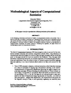
Let N2 be the average number of neighbors within two hops. As shown in Figure 4, two nodes become two-hop neighbors only if there is at least one common neighbor in the shaded area. The average number of nodes in the
In addition, the chances of unicast transmissions in either the UT or the DT states depend on three factors: (a) the number of one-hop neighbors of the source, (b) the number of one-hop neighbors of the destination, and (c) the distance between the source and destination.
shaded area is: 2
B(t) = 2ρr a(t) , where t t a(t) = arccos − 2 2
s
� �2 t . 1− 2
(3)
Thus, the probability of having at least one node in the shaded area is 1 − e−B(t) . Adding up all nodes covered by the ring (r, 2r) around the node, multiplied by the corresponding probability of becoming two-hop neighbors, the average number of two-hop neighbors of a node is: Z 2 � � n2 = ρπr2 2t 1 − e−B(t) dt . 1
Because the number of one-hop neighbors is N1 = ρπr2 , adding the average number of one-hop and twohop neighbors, we obtain the number of neighbors within two hops as: � Z 2 � � � 2t 1 − e−B(t) dt . N 2 = N 1 + n2 = N 1 1 +
S(t)
T (N ) =
∞ X
k=1
1 N k −N eN − 1 − N . e = k + 1 k! N eN
Note that k starts from 1 in the expression for T (N ), because a node with no contenders does not win at all. U (N ) is the probability that a node has at least one contender, which is simply
W (N ) is introduced to denote 1 (1 − e−N ) . N Because N2 denotes the average number of two-hop neighbors, which is the number of contenders for each node in HAMA, it follows that the probability that the node broadcasts is T (N2 ). Therefore, the channel access probability of a node in HAMA is the node activation cases in the broadcast state (BT): W (N ) = U (N ) − T (N ) = 1 −
pBT = T (N2 ) . In addition, HAMA provides two states for a node to transmit in the unicast mode (UT and DT). Overall, if node i transmits in the unicast state (UT and DT), node i must have at least one neighbor j, of which the probability is pu = U (N1 ) .
j
Figure 5. Unicast between two nodes.
First, we consider the probability of unicast transmissions from node i to node j in the UT state, in which case, node i contend with nodes residing in the combined onehop coverage of nodes i and j, as illustrated in Figure 5. Given that the transmission range is r and the distance between nodes i and j is tr (0 < t < 1), we denote the number of nodes within the combined coverage by k1 excluding nodes i and j, of which the average is S(t) = 2ρr2 [π − a(t)] . a(t) is defined in Eq. (3). Therefore, the probability of node i winning in the combined one-hop coverage is: p1 =
∞ X
k1 =0
1 S(t)k1 −S(t) W (S(t)) e = . k1 + 2 k1 ! S(t)
Furthermore, because node i cannot broadcast when it enters the UT state, there has to be at least one twohop neighbor with higher priority than node i outside the combined one-hop coverage in Figure 5. Denote the number of nodes outside the coverage by k2 , of which the average is N2 − S(t). The probability of node i losing outside the combined coverage is thus: p2 =
∞ X [N2 − S(t)]k2
k2 =1
U (N ) = 1 − e−N .
tr
r
1
For convenience, symbol T (N ), U (N ) and W (N ) are introduced to denote three probabilities when the average number of contenders is N . T (N ) denotes the probability of a node winning among its contenders. Because the number of contenders follows Poisson distribution with mean N , and that all nodes have equal chances of winning, the probability T (N ) is the average over all possible numbers of the contenders:
i
A(t)
k2 !
e−(N2 −S(t))
k2 = W (N2 −S(t)) . k2 + 1
In all, the probability of node i transmitting in the UT state is: p3 = p1 · p2 =
W (N2 − S(t)) W (S(t)) . S(t)
The probability density function (PDF) of node j at position t is p(t) = 2t. Therefore, integrating p3 on t over the range (0, 1) with PDF p(t) = 2t gives the average probability of node i becoming a transmitter in UT state: Z 1 Z 1 W (N2 − S(t)) W (S(t)) pUT = dt . p3 2tdt = 2t S(t) 0 0 Second, we consider the probability of unicast transmissions from node i to node j in the DT state. We denote the number of one-hop neighbors of node j by k3 , excluding nodes i and j, of which the average is N1 . Then, node j requires the lowest priority among its k3 neighbors to be a drain, and node i requires the
∞ X N1k3 −N1 1 1 T (N1 ) p4 = . e = k3 ! k3 + 2 k3 + 1 N1 k3 =0
In addition, node i has to lose to nodes residing in the side lobe, marked by A(t) in Figure 5. Otherwise, node i would enter the UT state. Denote the number of nodes in the side lobe by k4 , of which the average is i hπ − a(t) . A(t) = 2ρr2 2 The probability of node i losing in the side lobe is thus ∞ X A(t)k4 −A(t) k4 p5 = e = W (A(t)) . k4 ! k4 + 1
ρ=0.0001 Node/Square Area 0.4
Channel Access Probability
highest priority to transmit to node j, of which the average probability over all possible values of k3 is:
0
2t W (A(t)) dt .
0
In summary, the average channel access probability of a node in the network is the chance of becoming a transmitter in the three mutually exclusive broadcast or unicast states (BT, UT or DT), which is given by qHAM A = pBT + pu (pU T + pDT ) = T (N2 ) + U (N1 ) ·
+
Z
0
1
2t
�
T (N1 ) N1
Z
1
2t W (A(t)) dt
0
W (N2 − S(t)) W (S(t)) dt S(t)
�
0
100
200 300 400 Transmission Range
500
Figure 6. Channel access probability of NAMA, HAMA, PAMA and LAMA.
(4)
.
The above analyses for HAMA have made four simplifications. Firstly, we assumed that the number of two-hop neighbors also follows Poisson distribution, just like that of one-hop neighbors. Secondly, we let N2 − S(t) ≥ 0 even though N2 may be smaller than S(t) when the transmission range r is small. Thirdly, only one neighbor j is considered when making node i to become a unicast transmitter in the DT or the UT state, although node i may have multiple chances to do so owning to other onehop neighbors. The results of the simulation experiments reported in Section V validate these approximations. B. Comparison among NAMA, HAMA, PAMA and LAMA In [21], we have made similar analysis for other channel access scheduling protocols, namely NAMA (node activation multiple access), PAMA (pair-wise activation multiple access) and LAMA (link activation multiple access). We compare these protocols with HAMA side by side by in a simulated ad hoc network scenario, in
Channel Access Probability
T (N1 ) W (A(t)) . N1
T (N1 ) N1
0.1
ρ=0.0001 Node/Square Area
2
Using the PDF p(t) = 2t for node j at position t, the integration of the above result over range (0, 1) gives the average probability of node i entering the DT state, denoted by pDT : Z 1 Z 1 p6 2tdt =
0.2
10
In all, the probability of node i entering the DT state for transmission to node j is the product of p4 and p5 :
pDT =
0.3
0
k4 =1
p6 = p4 · p5 =
NAMA HAMA PAMA LAMA
HAMA / NAMA PAMA / NAMA LAMA / NAMA
1
10
0
10
0
100
200 300 400 Transmission Range
500
Figure 7. Channel access probability ratio of HAMA, PAMA and LAMA to NAMA.
which the network density is ρ = 0.0001, equivalent to placing 100 nodes on a 1000 × 1000 square plane. The relation between transmission range and the channel access probability of a node in NAMA, HAMA, PAMA and LAMA is shown in Figure 6. Because a node barely has any neighbor in a multihop network when the node transmission range is too short, Figure 6 shows that the system throughput is close to none at around zero transmission range, but it increases quickly to the peak when the transmission range covers around one neighbor on the average, except for that of PAMA, which is an upper bound. Then network throughput drops when more and more neighbors are contacted and the contention level increases. Figure 7 shows the performance ratio of the channel access probabilities of HAMA, PAMA and LAMA to that NAMA. At shorter transmission ranges, HAMA, PAMA and LAMA performs very similar to NAMA, because nodes are sparsely connected, and node or link activations are similar to broadcasting. When transmission range increases, HAMA, LAMA and PAMA obtains more and more opportunities to leverage its unicast capability and the relative throughput also increases more than three times that of NAMA. C. Comparison with CSMA and CSMA/CA We compare the throughput of HAMA with that of idealized CSMA and CSMA/CA protocols [19], [20]. We
λ=
p′ ldata ldata = 1/p′ + ldata 1 + p′ ldata
because the average interval between successive transmissions follows Geometric distribution with parameter p′ . The network throughput is measured by the successful data packet transmission rate within the one-hop neighborhood of a node in [19], [20], instead of the whole network. Therefore, the comparable network throughput in HAMA is the sum of the packet transmissions by each node and all of its one-hop neighbors. We reuse the symbol N in this section to represent the number of onehop neighbors of a node, which is the same as N1 defined in Section IV-A. Because every node is assigned the same load λ, and has the same channel access probability (qHAMA ), the throughput of HAMA becomes SHAMA = N · min(λ, qHAMA ) . Figure 8 compares the throughput attributes of HAMA, NAMA, the idealized CSMA [19], and CSMA/CA [20] with different numbers of one-hop neighbors in two scenarios. The first scenario assumes that data packets last for ldata = 100 time slots in CSMA and CSMA/CA, and the second assumes a 10-time-slot packet size average. The network throughput decreases when a node has more contenders in NAMA, CSMA and CSMA/CA, which is not true for HAMA. In addition, HAMA and NAMA provide higher throughput than CSMA and
Data Packet Size=100
Data Packet Size=10
1
1 0.8 Throughput S
0.8 Throughput S
consider only unicast transmissions, because CSMA/CA does not support collision-free broadcast. Scheduled access protocols are modeled differently from CSMA and CSMA/CA. In time-division scheduled channel access, a time slot can carry a complete data packet, while the time slot for CSMA and CSMA/CA only lasts for the duration of a channel round-trip propagation delay, and multiple time slots are used to transmit a data packet once the channel is successfully acquired. In addition, Wang et al. [20] and Wu et al. [19] assumed a heavily loaded scenario in which a node always has a data packet during the channel access, which is not true for the throughput analysis of HAMA, because using the heavy load approximation would always result in the maximum network capacity. The probability of channel access at each time slot in CSMA and CSMA/CA is parameterized by the symbol p′ . For comparison purposes, we assume that every attempt to access the channel in CSMA or CSMA/CA is an indication of a packet arrival at the node. Though the attempt may not succeed in CSMA and CSMA/CA due to packet or RTS/CTS signal collisions in the common channel, and end up dropping the packet, conflict-free scheduling protocols can always deliver the packet if it is offered to the channel. In addition, we assume that no packet arrives during the packet transmission. Accordingly, the traffic load for a node is equivalent to the portion of time for transmissions at the node. Denote the average packet size as ldata , the traffic load for a node is given by
0.6 0.4 0.2
0.6
CSMA (N=3) CSMA (N=10) CSMA/CA (N=3) CSMA/CA (N=10) HAMA (N=3) HAMA (N=10) NAMA (N=3) NAMA (N=10)
0.4 0.2
0
0
0
0
10 ′
Channel Access Probability p
Figure 8. CSMA/CA.
10 Channel Access Probability p′
Comparison between HAMA, NAMA and CSMA,
CSMA/CA, because all transmissions are collision-free even when the network is heavily loaded. In contrast to the critical role of packet size in the throughput of CSMA and CSMA/CA, it is almost irrelevant in that of scheduled approaches, except for shifting the points of reaching the network capacity. V. S IMULATIONS The delay and throughput attributes of HAMA are studied in comparison with those of NAMA, LAMA, PAMA and UxDMA [9] in two simulation scenarios: fully connected networks with different numbers of nodes, and multihop networks with different radio transmission ranges. In the simulations, we use the normalized packets per time slot for both arrival rates and throughput. This metric can be translated into concrete throughput metrics, such as Mbps (megabits per second), if the time slot sizes and the channel bandwidth are instantiated. Because the channel access protocols based on NCR have different capabilities regarding broadcast and unicast, we only simulate unicast traffic at each node in all protocols. All nodes have the same load, and the destinations of the unicast packets at each node are evenly distributed over all one-hop neighbors. In addition, the simulations are guided by the following parameters and behavior: • The network topologies remain static during the simulations to examine the performance of the scheduling algorithms only. • Signal propagation in the channel follows the freespace model and the effective range of the radio is determined by the power level of the radio. Radiation energy outside the effective transmission range of the radio is considered negligible interference to other communications. All radios have the same transmission range. • Each node has an unlimited buffer for data packets. • 30 pseudo-noise codes are available for code assignments, i.e., |Cpn | = 30. • Packet arrivals are modeled as Poisson arrivals. Only one packet can be transmitted in a time slot. • The duration of the simulation is 100,000 time slots, long enough to collect the metrics of interests. For comparison purposes, we have also implemented UxDMA, the graph coloring algorithm for static network
2 Nodes
4
5 Nodes
80 60 40 20
30
20
10
1
2
50
250
Delay T (Time Slots)
0
0.05 0.1 0.15 Arrival Rate λ (Pkt/Slot)
0.2
0.02 0.04 0.06 0.08 Arrival Rate λ (Pkt/Slot)
0.1
2
3
4
100 Nodes Tx 200
150
100
50
0
0
100
0
250 200 150 100 50
150
0.02 0.04 0.06 0.08 Arrival Rate λ (Pkt/Slot)
0
0.1
0
100 Nodes Tx 300
50 0
1
300 HAMA Broadcast HAMA Unicast NAMA Broadcast UxDMA Broadcast
200
0
0.01 0.02 0.03 0.04 Arrival Rate λ (Pkt/Slot)
0.05
Figure 10. Average packet delays in fully-connected networks
Simulations were carried out in four configurations in the fully connected scenario: 2-, 5-, 10-, 20-node networks, to manifest the effects of different contention levels. Figure 9 shows the maximum throughput of each protocol in fully-connected networks. Except for PAMA and UxDMA-PAMA, the maximum throughput of every other protocol is one because their contention resolutions are based on the node priorities, and only one node is activated in each time slot. Because PAMA schedules link activations based on link priorities, multiple links can be activated on different codes in the fully-connected networks, and the channel capacity is greater in PAMA than in the other protocols. Figure 10 shows the average delay of data packets in NAMA, LAMA and PAMA with their corresponding UxDMA counterparts, and HAMA with regard to different loads on each node in fully-connected networks. NAMA, UxDMA-NAMA, LAMA, UxDMA-LAMA and HAMA have the same delay characteristic, because of the
0.04
700 600
400 300 200 100 0
0.01 0.02 0.03 Arrival Rate λ (Pkt/Slot) 100 Nodes Tx 400
500
Delay T (Time Slots)
Delay T (Time Slots)
200
50
10
0
4
Delay T (Time Slots)
0
20 Nodes 300
100
20
100 Nodes Tx 100
10 Nodes 250
150
30
Figure 11. Packet throughput in multihop networks
100
0
0.5
HAMA Analysis
HAMA Analysis
3
Delay T (Time Slots)
0.1 0.2 0.3 0.4 Arrival Rate λ (Pkt/Slot)
4
150
Delay T (Time Slots)
0
3
Transmission Range=400
200 0
2
40
0
Delay T (Time Slots)
Delay T (Time Slots)
200 HAMA Broadcast HAMA Unicast NAMA Broadcast UxDMA Broadcast
1
Transmission Range=300 40
Figure 9. Packet throughput in fully-connected networks
100
0
4
HAMA Analysis
3
3
Analysis UxDMA
2
2
10
NAMA Analysis UxDMA
UxDMA PAMA 1
1
20
UxDMA
0
4
HAMA
2
0
30
NAMA Analysis UxDMA
3
4
10
Throughput S (Packet/Slot)
2
6
20
HAMA Analysis
1
8
Throughput S (Packet/Slot)
0
10
LAMA UxDMA
1
HAMA
2
LAMA UxDMA
3
12
NAMA UxDMA
PAMA
4
Throughput S (Packet/Slot)
UxDMA
5
NAMA UxDMA
Throughput S (Packet/Slot)
6
30
Throughput S (Packet/Slot)
Transmission Range=400
PAMA Analysis UxDMA
4
PAMA Analysis UxDMA
3
PAMA Analysis UxDMA
HAMA
NAMA UxDMA
LAMA UxDMA 2
LAMA Analysis
Transmission Range=300
1
UxDMA
0
4
UxDMA
3
Transmission Range=200 40
LAMA Analysis
2
Transmission Range=100 40
NAMA Analysis UxDMA
1
1 0.5
NAMA Analysis UxDMA
0
2 1.5
Throughput S (Packet/Slot)
0.5
2.5
PAMA UxDMA
Throughput S (Packet/Slot)
HAMA
PAMA UxDMA
1
LAMA UxDMA
NAMA UxDMA
Throughput S (Packet/Slot)
1.5
PAMA
Transmission Range=200 3
LAMA Analysis UxDMA
Transmission Range=100 2
same throughput is achieved in these protocols. PAMA and UxDMA-PAMA can sustain higher loads and have longer “tails” in the delay curves. However, because the number of contenders for each link is more than the number of nodes, the contention level is higher for each link than for each node. Therefore, packets have higher starting delay in PAMA than other NCR-based protocols.
LAMA Analysis
topologies, with different constraint sets with regard to NAMA, LAMA and PAMA.
500 400 300 200 100
0
0.005 0.01 0.015 Arrival Rate λ (Pkt/Slot)
0
0
0.002 0.004 0.006 0.008 Arrival Rate λ (Pkt/Slot)
0.01
Figure 12. Average packet delays in multihop networks
Figure 11 and 12 show the throughput and the average packet delay of NAMA, LAMA, PAMA, HAMA and the UxDMA variations. Except for the ad hoc network generated using transmission range one hundred meters in Figure 11, UxDMA always outperforms its NCR-based counterparts — NAMA, LAMA and PAMA at various levels. For example, UxDMA-NAMA is only slightly better than NAMA in all cases, and UxDMA-PAMA is 10-30% better than PAMA. LAMA is comparatively the worst, with much lower throughput than its counterpart UxDMALAMA. One interesting point is the similarity between the throughput of LAMA and HAMA, which has been shown by Figure 8 as well, even though they have different
code assignment schemes and transmission schedules. Especially, the network throughput analyses of NAMA, LAMA, PAMA and HAMA Section IV is compared with the corresponding protocols in the simulations. The analytical results fits well with the simulations results. Note that the analysis bars with regard to PAMA and LAMA are the upper bounds, although the analysis of LAMA is very close to the simulation results. VI. C ONCLUSION We have introduced HAMA, a new distributed channel access scheduling protocol that dynamically determines the node- and link-activation schedule for both broadcast and unicast traffic. HAMA is remarkably simple, requires only two-hop neighborhood information, and avoids the complexities of prior conflict-free scheduling approaches that demand global topology information. The performance of HAMA was compared by analyses or simulations with that of other similar approaches, namely NAMA, LAMA and PAMA, as well as with that of idealized CSMA CSMA/CA and UxDMA. The results of our analyses clearly show that HAMA is far more effective, and renders comparable performance to that of UxDMA without requiring to maintain complete topology information at each node. As such, HAMA constitutes the most effective protocol for conflict-free channel access that does not require complete topology information. R EFERENCES [1] L. Kleinrock and F. Tobagi, “Packet switching in radio channels. I. Carrier sense multiple-access modes and their throughputdelay characteristics,” IEEE Transactions on Communications, vol. 23(12), pp. 1400–16, Dec 1975. [2] B. Crow, I. Widjaja, L. Kim, and P. Sakai, “IEEE 802.11 Wireless Local Area Networks,” IEEE Communications Magazine, vol. 35, no. 9, pp. 116–26, Sept 1997. [3] I. Cidon and M. Sidi, “Distributed assignment algorithms for multihop packet radio networks,” IEEE Transactions on Computers, vol. 38, no. 10, pp. 1353–61, Oct 1989. [4] Z. Tang and J. Garcia-Luna-Aceves, “A Protocol for TopologyDependent Transmission Scheduling,” in Proc. IEEE Wireless Communications and Networking Conference 1999 (WCNC 99), Sep. 21–24 1999. [5] C. Zhu and M. Corson, “A five-phase reservation protocol (FPRP) for mobile ad hoc networks,” in Proc. of IEEE Conference on Computer Communications (INFOCOM), vol. 1(2), Mar. 29-Apr. 2 1998, pp. 322–31. [6] A. Ephremides and T. Truong, “Scheduling broadcasts in multihop radio networks,” IEEE Transactions on Communications, vol. 38, no. 4, pp. 456–60, Apr. 1990. [7] S. Even, O. Goldreich, S. Moran, and P. Tong, “On the NPcompleteness of certain network testing problems,” Networks, vol. 14, no. 1, pp. 1–24, Mar. 1984. [8] R. Ramaswami and K. Parhi, “Distributed scheduling of broadcasts in a radio network,” in Proc. of IEEE Conference on Computer Communications (INFOCOM), vol. 2(3), Apr. 23-27 1989, pp. 497–504. [9] R. Ramanathan, “A unified framework and algorithm for channel assignment in wireless networks,” Wireless Networks, vol. 5, no. 2, pp. 81–94, 1999. [10] I. Chlamtac, A. Farago, and H. Zhang, “Time-spread multipleaccess (TSMA) protocols for multihop mobile radio networks,” IEEE/ACM Transactions on Networking, vol. 6, no. 5, pp. 804– 12, Dec. 1997. [11] J. Ju and V. Li, “An optimal topology-transparent scheduling method in multihop packet radio networks,” IEEE/ACM Transactions on Networking, vol. 6, no. 3, pp. 298–306, June 1998.
[12] R. Krishnan and J. Sterbenz, “An Evaluation of the TSMA Protocol as a Control Channel Mechanism in MMWN,” BBN Technical No. 1279, Apr. 26 2000. [13] L. Bao and J. Garcia-Luna-Aceves, “A New Approach to Channel Access Scheduling for Ad Hoc Networks,” in Proc. ACM Seventh Annual International Conference on Mobile Computing and networking, Rome, Italy, Jul. 16-21 2001. [14] ——, “Transmission Scheduling in Ad Hoc Networks with Directional Antennas,” in Proc. ACM Eighth Annual International Conference on Mobile Computing and networking, Sep. 23-28 2002. [15] D. Bertsekas and R. Gallager, Data Networks, 2nd edition. Englewood Cliffs, NJ: Prentice Hall, 1992. [16] T. Shepard, “A channel access scheme for large dense packet radio networks,” in ACM SIGCOMM ’96 Conference, Aug. 26-30 1996, pp. 219–30. [17] M. Joa-Ng and I. Lu, “Spread spectrum medium access protocol with collision avoidance in mobile ad-hoc wireless network,” in Proc. of IEEE Conference on Computer Communications (INFOCOM), Mar. 21-25 1999, pp. 776–83. [18] T. Makansi, “Trasmitter-Oriented Code Assignment for Multihop Radio Net-works,” IEEE Transactions on Communications, vol. 35, no. 12, pp. 1379–82, Dec. 1987. [19] L. Wu and P. K. Varshney, “Performance Analysis of CSMA and BTMA Protocols in Multihop Networks (I), Single Shannel Case,” Information Sciences, vol. 120(1-4), pp. 159–177, 1999. [20] Y. Wang and J. Garcia-Luna-Aceves, “Performance of Collision Avoidance Protocols in Single-Channel Ad Hoc Networks,” in Proc. of IEEE International Conference on Network Protocols (ICNP), Nov. 12-15 2002. [21] L. Bao and J. Garcia-Luna-Aceves, “Distributed Dynamic Channel Access Scheduling for Ad Hoc Networks,” Journal of Parallel and Distributed Computing, Special Issue on Wireless and Mobile Ad Hoc Networking and Computing, 2002. Lichun Bao received the B.S. degree in computer science from the University of Science and Technology of China, Hefei, China, in 1994, the M.E. degree in computer engineering from Tsinghua University, Beijing, China, in 1997, and the Ph.D. degree in computer science from the University of California, Santa Cruz, CA, in 2002. He is an Assistant Professor of Computer Science at the University of California, Irvine (UCI). J.J. Garcia-Luna-Aceves holds the Jack Baskin Chair of Computer Engineering at the University of California, Santa Cruz (UCSC), and is a Principal Scientist at the Palo Alto Research Center (PARC). Prior to joining UCSC in 1993, he was a Center Director at SRI International (SRI) in Menlo Park, California. He has been a Visiting Professor at Sun Laboratories and a Principal of Protocol Design at Nokia. Dr. Garcia-Luna-Aceves has published a book, more than 370 papers, and 26 U.S. patents. He has directed 26 Ph.D. theses and 22 M.S. theses since he joined UCSC in 1993. He has been the General Chair of the ACM MobiCom 2008 Conference; the General Chair of the IEEE SECON 2005 Conference; Program Co-Chair of ACM MobiHoc 2002 and ACM MobiCom 2000; Chair of the ACM SIG Multimedia; General Chair of ACM Multimedia ’93 and ACM SIGCOMM ’88; and Program Chair of IEEE MULTIMEDIA ’92, ACM SIGCOMM ’87, and ACM SIGCOMM ’86. He has served in the IEEE Internet Technology Award Committee, the IEEE Richard W. Hamming Medal Committee, and the National Research Council Panel on Digitization and Communications Science of the Army Research Laboratory Technical Assessment Board. He has been on the editorial boards of the IEEE/ACM Transactions on Networking, the Multimedia Systems Journal, and the Journal of High Speed Networks. He is a Fellow of the IEEE and is listed in Marquis Who’s Who in America and Who’s Who in The World. He is the co-recipient of the IEEE Fred W. Ellersick MILCOM Award for best unclassified paper at IEEE MILCOM 2008. He is also co-recipient of Best Paper Awards at the IEEE MILCOM 2008, IEEE MASS 2008, SPECTS 2007, IFIP Networking 2007, and IEEE MASS 2005 conferences, and of the Best Student Paper Award of the 1998 IEEE International Conference on Systems, Man, and Cybernetics. He received the SRI International Exceptional-Achievement Award in 1985 and 1989.