Physica A 391 (2012) 4088–4099
Contents lists available at SciVerse ScienceDirect
Physica A journal homepage: www.elsevier.com/locate/physa
Langevin simulation of scalar fields: Additive and multiplicative noises and lattice renormalization N.C. Cassol-Seewald a , R.L.S. Farias b,∗ , E.S. Fraga c , G. Krein a , Rudnei O. Ramos d a b
Instituto de Física Teórica, Universidade Estadual Paulista, Rua Dr. Bento Teobaldo Ferraz, 271 - Bloco II, 01140-070 São Paulo, SP, Brazil Departamento de Ciências Naturais, Universidade Federal de São João Del Rei, 36301-000 São João Del Rei, MG, Brazil
c
Instituto de Física, Universidade Federal do Rio de Janeiro, 21941-972 Rio de Janeiro, RJ, Brazil
d
Departamento de Física Teórica, Universidade do Estado do Rio de Janeiro, 20550-013 Rio de Janeiro, RJ, Brazil
article
info
Article history: Received 6 December 2011 Received in revised form 8 February 2012 Available online 1 April 2012 Keywords: Langevin dynamics Lattice renormalization Multiplicative noise
abstract We consider the Langevin lattice dynamics for a spontaneously broken λφ 4 scalar field theory where both additive and multiplicative noise terms are incorporated. The lattice renormalization for the corresponding stochastic Ginzburg–Landau–Langevin and the subtleties related to the multiplicative noise are investigated. © 2012 Elsevier B.V. All rights reserved.
1. Introduction The relevance of mathematical methods of quantum field theory for statistical physics was recognized in the early seventies, particularly in the investigation of equilibrium phase transitions and critical phenomena. Renormalization theory, originally linked with the removal of infinities in perturbative calculations in quantum field theory, turned out to be a key element in the understanding of critical phenomena [1]. Functional integrals, Feynman diagrams and loop expansions are an integral part of the mathematical methods used presently in statistical physics — Ref. [2] is an excellent introductory text on concepts and methods of field theory in the quantum and statistical domains. Likewise, a large class of dynamic critical phenomena associated with time-dependent fluctuations about equilibrium states, naturally described in terms of stochastic partial differential equations [3,4], can also be formulated in terms of functional integrals and therefore are equivalently described by field theories [5]. Among the variety of phenomena associated with the dynamics of phase transitions, phase ordering [6] seems to be of particular importance for the understanding of the time scales governing the equilibration of systems driven out of equilibrium. The influence of the presence of an environment on the dynamics of particles and fields is encoded ‘‘macroscopically’’ in attributes that enter stochastic evolution equations, usually in the form of dissipation and noise terms. Relevant time scales for different stages of phase conversion can depend dramatically on the details of these attributes. Noise terms, in particular, introduce difficulties in the numerical simulation of the evolution equations; difficulties related to the well-known Rayleigh–Jeans catastrophe in classical field theory [7]. The present paper is concerned with the use of field-theoretic renormalization methods to control such catastrophe.
∗
Corresponding author. Tel.: +55 32 3373 4535; fax: +55 32 3379 2483. E-mail addresses:
[email protected] (N.C. Cassol-Seewald),
[email protected],
[email protected] (R.L.S. Farias),
[email protected] (E.S. Fraga),
[email protected] (G. Krein),
[email protected] (R.O. Ramos). 0378-4371/$ – see front matter © 2012 Elsevier B.V. All rights reserved. doi:10.1016/j.physa.2012.03.026
N.C. Cassol-Seewald et al. / Physica A 391 (2012) 4088–4099
4089
A typical dynamical equation describing phase conversion is of the form of a Ginzburg–Landau–Langevin (GLL) equation [8]:
∂ 2ϕ ′ − ∇ 2 ϕ + η ϕ˙ + Veff (ϕ) = ξ (x, t ), (1) ∂t2 ′ where ϕ is a real scalar field, function of time and space variables, Veff (ϕ) is the field derivative of a Ginzburg–Landau effective potential and η, which can be seen as a response coefficient that defines time scales for the system and encodes the intensity of dissipation, is usually taken to be a function of temperature only, η = η(T ). The function ξ (x, t ) represents τ
a stochastic (noise) force, assumed Gaussian and white, so that
⟨ξ (x, t )⟩ξ = 0,
⟨ξ (x, t )ξ (x′ , t ′ )⟩ξ = 2 ηT δ(x − x′ )δ(t − t ′ ),
(2)
in conformity with the fluctuation–dissipation theorem. The condensate ⟨ϕ⟩ξ plays the role of the order parameter, where ⟨· · ·⟩ξ means average over noise realizations. The second order time derivative in Eq. (1) appears naturally in relativistic field theories [9,10] or when causality is incorporated via memory functions [11,12] in the otherwise purely diffusive, first-order evolution equations [3,8]. However, a more complete, microscopic field-theory description of nonequilibrium dissipative dynamics [13] shows that the complete form for the effective GLL equation of motion can lead to much more complicated scenarios than the one described by Eq. (1), depending on the allowed interaction terms involving ϕ . In general, there will be nonlocal (non-Markovian) dissipation and colored noise, as well as the possibility of field-dependent (multiplicative) noise terms ∼ϕ ξ accompanied by density-dependent dissipation terms. Another typical example is provided by stochastic Gross–Pitaevskii (SGP) equations [14,15] that incorporate thermal and quantum fluctuations of a Bose–Einstein condensate (BEC) on the traditional mean-field equation [16]. Such a stochastic equation can be derived from a microscopic inter-atomic Hamiltonian via the closed-time-path Schwinger–Keldysh effective action formalism [13]. In fact, on very general physical grounds, one expects that dissipation effects should depend on the local density ∼ϕ 2 ϕ˙ and, accordingly, the noise term should contain a multiplicative piece ∼ϕξ . The typical term coming from fluctuations in the equation of motion for ϕ will be a functional of the form [13]
F [ϕ(x)] = ϕ(x)
d4 x′ ϕ 2 (x′ )K1 (x, x′ ) +
d4 x′ ϕ(x′ )K2 (x, x′ ),
(3)
where K1 (x, x′ ) and K2 (x, x′ ) are nonlocal kernels expressed in terms of retarded Green’s functions and whose explicit form depends on the detailed nature of the interactions involving ϕ . Explicit treatments for these nonlocal kernels show that under appropriate conditions one is justified to express the effective equation of motion for ϕ in a local form (see e.g. Ref. [17] and references therein). The existence of these additional terms in the GLL equation will, of course, play an important role in the dynamics of the formation of condensates. For instance, it was shown that the effects of multiplicative noise are rather significant in the Kibble–Zurek scenario of defect formation in one spatial dimension [18]. Although in the literature there are many different approaches for studying the nonequilibrium dynamics in field theory [19–21], the use of stochastic Langevin-like equations of motion is still a simpler and more direct approach in many different contexts in statistical physics and field theory in general. For example, some of us have considered the effects of dissipation in the scenario of explosive spinodal decomposition: the rapid growth of unstable modes following a quench into the two-phase region of the quantum chromodynamics (QCD) chiral transition in the simplest fashion [22]. Using a phenomenological Langevin description inspired by microscopic nonequilibrium field theory results [10,23,24], the time evolution of the order parameter in a chiral effective model [25] was investigated. Real-time (3 + 1)-dimensional lattice simulations for the behavior of the inhomogeneous chiral fields were performed, and it was shown that the effects of dissipation could be dramatic in spite of the very conservative assumptions that were made. Later, analogous but even stronger effects were obtained in the case of the deconfining transition of SU (2) pure gauge theories using the same approach [26,27]. Recent work in these directions by a different group can be found in Refs. [28,29]. In the present paper we consider the nonequilibrium dynamics of the formation of a condensate in a spontaneously broken λϕ 4 scalar field theory within an improved Langevin framework which includes the effects of multiplicative noise and density-dependent dissipation terms. The corresponding stochastic GLL equation can be thought of as a generalization of the results of Ref. [10] to the case of broken symmetry. The time evolution for the formation of the condensate, under the influence of additive and multiplicative noise terms, is solved numerically on a (3 + 1)-dimensional lattice. Particular attention is devoted to the renormalization of the stochastic GLL equation in order to obtain lattice-independent equilibrium results. The paper is organized as follows. In Section 2 the proper lattice renormalization of the GLL, in order to achieve equilibrium solutions that are independent of lattice spacing, is addressed. In Section 3 the question of time discretization for a GLL with multiplicative noise is discussed. In Section 4 we show the results of our lattice simulations to study the behavior of the condensate. Section 5 contains our conclusions and perspectives. 2. Stochastic GLL equations In our study, we consider an extended GLL equation, incorporating additive and multiplicative noise terms. The time evolution of the field ϕ(x, t ) at each point in space, which will determine the approach of the condensate ⟨ϕ⟩ to its
4090
N.C. Cassol-Seewald et al. / Physica A 391 (2012) 4088–4099
equilibrium value will be dictated by the following equation:
∂ϕ ∂ 2ϕ ′ − ∇ 2 ϕ + η1 ϕ 2 + η2 + Veff (ϕ) = ξ1 (x, t ) ϕ + ξ2 (x, t ), (4) ∂t2 ∂t where the dissipation coefficients η1 and η2 can be seen as response coefficients that define time scales for the system and encode the intensity of dissipation. The functions ξ1 (x, t ) and ξ2 (x, t ) represent stochastic (noise) forces, assumed Gaussian and white, as in Eq. (2). The motivation for Eq. (4) stems largely from explicit microscopic derivations of the effective equation of motion for nonequilibrium quantum fields, where this type of equation emerges naturally. We refer the interested reader to Refs. [10,13] for more details. 2.1. Lattice renormalization Analytic solutions of Eq. (4) are achievable only in very special situations (for the case of zero spatial dimensions, see e.g. Ref. [30]), like in a linear approximation to Veff (ϕ), usually valid only at short times. Complete solutions describing the evolution of the system to equilibrium can be obtained only through extensive numerical simulations. In general, numerical simulations are performed on a discrete spatial lattice of finite length under periodic boundary conditions. However, in performing lattice simulations of Eq. (4), one should be careful in preserving the lattice-spacing independence of the results, especially when one is concerned with the behavior of the system in the continuum limit. The equilibrium probability distribution for the field configurations φ that are solutions of Eq. (4) is Peq [φ] = e−S [φ] , where S [φ] is the Euclidean action. The corresponding partition function is given by the path integral
Z [φ] =
D φ e−S [φ] .
(5)
The calculation of expectation values and correlation functions of φ with this partition function leads to ultraviolet divergences. In the presence of thermal noise, short and long wavelength modes are mixed during the dynamics, yielding an unphysical lattice spacing sensitivity. Such a lattice spacing sensitivity is also present in the numerical simulation of SGP equations [31,32]. The issue of obtaining robust results, as well as the correct ultraviolet behavior, in performing Langevin dynamics was discussed by several authors [33–38]. The problem, which is not a priori evident in the Langevin formulation, is related to the well-known Rayleigh–Jeans ultraviolet catastrophe in classical field theory [7]. The dynamics dictated by Eq. (4) is classical, and is ill-defined for large momenta. These a priori lattice divergences can be eliminated by renormalizing the potential Veff through the addition of appropriate counterterms (notice that these divergences are completely unrelated to the usual ones of the quantum theory). Since the divergent terms are all perturbative, one can identify the appropriate diagrams and subtract their result computed within the classical theory. Since the theory in three-dimensions is super-renormalizable, only a mass renormalization is required. We only require, then, a renormalization of the mass parameter m20 in Veff (ϕ). Using such a renormalized potential in Eq. (4) leads to equilibrium solutions ϕ that are independent of the lattice spacing as we are going to explicitly show below. In practice, this lattice renormalization procedure corresponds to adding finite-temperature counterterms to the original potential Veff (ϕ), which guarantees the correct short-wavelength behavior of the discrete theory as was originally shown by the authors of Ref. [39] within the framework of dimensional reduction in a different context. In order to define the notation and the procedure to calculate the loop expansion of the effective potential [40], we first consider the theory in the continuum and switch to the lattice when calculating the loop integrals. 2.2. The classical field effective potential in the continuum: Loop corrections The calculation of the classical three-dimensional loop corrections to the potential starts as usual by introducing a constant field ϕ through the transformation
φ → φ + ϕ,
(6)
and considering the action Sˆ [ϕ; φ] ≡ S [ϕ + φ] − S [ϕ] −
∂ S [φ] d xφ ∂φ
3
.
(7)
φ=ϕ
Next, the quadratic terms in Sˆ are collected in a ‘‘free’’ action Sˆ2 , and the remaining terms in an interacting action, SˆI . Then, the effective classical field potential is defined by the expression e−β V Veff [ϕ] = e−β V V [ϕ]
ˆ
D φ e−S [ϕ;φ] ,
(8)
N.C. Cassol-Seewald et al. / Physica A 391 (2012) 4088–4099
4091
where V is the three-dimensional volume. From this expression, one obtains for Veff [ϕ]
Veff [ϕ] = V [ϕ] −
1
ˆ
D φ e−S2 [ϕ;φ] −
ln
βV
1
βV
ˆ
ln⟨e−SI [ϕ,φ] ⟩,
(9)
where ˆ
ˆ
D φ e−S2 [ϕ;φ] e−SI [ϕ;φ]
ˆ
⟨e−SI [ϕ,φ] ⟩ =
D φ e−Sˆ2 [ϕ;φ]
.
(10)
The final step is the determination of ϕ through d Veff [ϕ]
= 0.
dϕ
(11)
For a bare potential of the form V = −m20 φ 2 /2 + λφ 4 /4!, the action Sˆ2 [ϕ; φ] is given by Sˆ2 [ϕ; φ] = β
1 1 − φ∇ 2 φ + m2 φ 2 ,
d3 x
2
2
(12)
where m2 = −m20 +
1 2
λϕ 2 .
(13)
Since ϕ is constant, the first functional integral in Eq. (9) can be easily performed in momentum space, with the result
1
βV
−Sˆ2 [ϕ;φ]
Dφ e
ln
=−
T 2
ln G−1 [ϕ; k2 ],
(14)
k
where G−1 [ϕ; k2 ] is the inverse of the three-dimensional (classical field) propagator
G[ϕ; k2 ] = and
≡
k
d3 k
1 k2 + m2
,
(15)
. The next divergent contribution comes from the two-loop correction to the mass, which will require SˆI ,
(2π)3
SˆI [ϕ; φ] = β
d3 x
1 1 − κφ 3 + λφ 4 , 3 4!
(16)
ˆ with κ = − 21 λϕ . Expansion of e−SI in Eq. (9) gives the two-loop divergent contribution, that we will denote as H [ϕ] and defined by
1
ˆ
βV
ln⟨e−SI [ϕ,φ] ⟩t wo−loop =
T2
1
κ
2 6 H [ϕ],
(17)
G[ϕ; k2 ] G[ϕ; q2 ] G[ϕ; (k + q)2 ].
(18)
2
3
where H [ϕ] =
1
6V
= k
d3 x d3 y⟨φ 3 (x)φ 3 (y)⟩
q
Now, the total divergent part of Veff [ϕ] is obtained from
d2 Veff [ϕ] dϕ 2
= div.terms
λT 2
Idiv [ϕ] −
λ2 T 2 6
Hdiv [ϕ],
(19)
with
G[ϕ; k2 ],
I [ϕ] =
(20)
k
where Idiv [ϕ] and Hdiv [ϕ] represent the divergent parts of I [ϕ] and H [ϕ]. Notice that the derivatives of H [ϕ] with respect to ϕ lead to finite integrals and hence are irrelevant here. The evaluation of the divergent parts of I and H requires a regularization scheme. Since we simulate our GLL equations on a cubic lattice, we shall evaluate these divergent parts by calculating the effective potential on the lattice.
4092
N.C. Cassol-Seewald et al. / Physica A 391 (2012) 4088–4099
2.3. The counterterms for the classical field potential on the lattice Here we consider the theory on a cubic lattice of volume V = L3 , with L = Na, where a is the lattice spacing and N is the number of lattice spacings. The coordinates xi of the lattice sites are such that 0 ≤ xi ≤ a(N − 1). The Laplacian on the 2 lattice, ∇latt ≡ ∆, is defined as
∆φ(x) =
3 1
a2 i=1
φ(x + aˆi) − 2φ(x) + φ(x − aˆi) ,
(21)
where ˆi is the unit Cartesian vector indicating the three orthogonal directions of the square lattice. We also impose periodic boundary conditions (PBC) on the fields,
φ(x + aN ˆi) = φ(x),
(22)
and define the Fourier transform f˜ (k) of a function f (x) on the lattice as f˜ (k) = a3
e−ik·x f (x).
(23)
x
Because of the PBC, the allowed lattice momenta form the Brillouin zone B ki =
2π aN
ni ,
ni = 0, 1, 2, . . . , N − 1.
(24)
The inverse transform is given by f (x) =
1 V k ∈B
eik·x f˜ (k),
(25)
and the momentum summations over the Brillouin zone will be denoted by 1 V k ∈B
.
≡
(26)
k
Let us now consider the derivation of the effective potential on the lattice. The lattice action is given by
1 Slatt [φ] = a − φ ∆φ + V [φ] , 3
(27)
2
x
where V [ϕ] is the same as before. The derivation of the effective potential follows the same procedure as in the continuum, leading to expressions for the one-loop and two-loop divergent contributions as in Eqs. (18) and (20), but with k given by the sum over lattice momenta as indicated in Eq. (26). What remains to be determined is the lattice propagator corresponding to G. The lattice propagator Glatt can be obtained from the quadratic action Sˆ2 [ϕ; φ] on the lattice Sˆ2 latt [ϕ; φ] = a3
1 1 − φ ∆φ + m 2 φ 2 , x
2
(28)
2
with m2 given by Eq. (13). The lattice propagator Glatt [ϕ; x, y] is the inverse of −∆ + m2 , i.e.
a3
1 −∆ + m2 x,y Glatt [ϕ; x, y] = 3 δx,y , a
y
(29)
where δx,y is the Kronecker delta. Since ϕ is a constant field, the solution of this equation can be obtained using the Fourier transform of Glatt [ϕ; x, y], defined as Glatt [ϕ; x, y] =
eik·x Glatt [ϕ; k2 ].
(30)
k
Substituting this into Eq. (29), one obtains a2 Glatt [ϕ, k2 ] =
1
4 d(ϕ; n1 , n2 , n3 )
where
,
(31)
N.C. Cassol-Seewald et al. / Physica A 391 (2012) 4088–4099
a2
d(ϕ; n1 , n2 , n3 ) =
=
2a−2
4
3
4093
(1 − cos aki ) + m2
i=1
3
sin2 (π ni /N ) + (am/2)2 .
(32)
i =1
One can then write I [ϕ] for the one-loop divergent term as I [ϕ] =
N
1
1
d(ϕ; n1 , n2 , n3 ) n i =0
4aN 3
,
(33)
and the double sum in H [ϕ] for the two-loop divergent term as N −1
1
H [ϕ] =
1
d(ϕ; n1 , n2 , n3 ) d(ϕ; m1 , m2 , m3 ) ni ,mi =0
64N 6
×
1 d(ϕ; n1 + m1 , n2 + m2 , n3 + m3 )
.
(34)
The divergent parts of the sums above can be isolated in the limits of N → ∞ and a → 0. For example, in the one-loop term the sum in the limit of N → ∞ can be converted into an integral [39], π
1
I [ϕ] =
4aπ
3
0
d3 x
1 sin xi + (am/2)2 2
i
1
=
4a
∞
3 2 dα e−α(am) /4 e−α/2 I0 (α/2) ,
(35)
0
where I0 is the modified Bessel function. In the limit of a → 0, the divergent part of I [ϕ] is given by
Σ
Idiv [ϕ] =
4π a
,
(36)
where Σ is a constant defined by
Σ=
1
π2
+π/2 −π/2
d3 x
1 sin2 xi
≃ 3.1759.
(37)
i
It is important to remark here that for T < Tc it is crucial the use of Eq. (11) so that m2 < 0 in the above expressions. In a more demanding numerical computation, Hdiv [ϕ] can also be isolated, with the result [39] Hdiv [ϕ] =
1
16π 2
ln
6 aM
+ζ ,
(38)
where M is the renormalization scale and ζ ≃ 0.09 is another constant appearing in the integrals being evaluated numerically. The renormalized mass in the classical field perturbative loop expansion is obtained as in the case of quantum field theory, i.e. by subtracting the divergent parts of these graphs as indicated in Eq. (19):
−
1 2
m2 φ 2 → −
1 2 1 m + δ m2 φ 2 ≡ − m2R φ 2 , 2 2
(39)
where the mass counterterm is given by
δ m2 =
λT 2
Idiv [ϕ] −
λ2 T 2 6
Hdiv [ϕ].
(40)
Therefore, we add the following finite-temperature counterterms to our original potential:
2 λΣ T λ2 2 6 ϕ Vct = − + T ln +ζ . 8π a 96π 2 aM 2
(41)
Notice from the above equation that the dependence on the mass scale M of the lattice counterterm is only logarithmic. So, it turns out that results are only very weakly dependent on changes of the scale M. Of course, any change in the renormalization scale M can be compensated by corresponding changes in the renormalized parameters as also expected from the renormalization group theory; here only a change in the coefficient of the term proportional to ϕ 2 is required, as it is clear from Eq. (41).
4094
N.C. Cassol-Seewald et al. / Physica A 391 (2012) 4088–4099
3. Multiplicative noise and time discretization The equation to be solved on the lattice is given by Eq. (4). We solve the GLL equation on the lattice with periodic n boundary conditions (PBC). When we insert the system in a box, ϕ acquires a discrete form ϕijk , where t = n∆t with n = 0, 1, 2, . . . , x = ia, y = ja and z = ka, a being the lattice spacing a =
ϕ
=ϕ ;
ϕ
=ϕ
ϕ
=ϕ ;
n n n n N +1jk 1jk iN +1k i1k n n n N +1N +1k 11k N +1jN +1 n n n N +1N +1N +1 111 0jk n n n n ij0 ijN i00 iNN
ϕ
=ϕ
ϕ
ϕ
;
=ϕ ;
ϕ
n n ϕ00k = ϕNNk ;
=ϕ ;
ϕ
;
ϕ
n ijN +1
=ϕ
;
ϕ
n 0j0
Using PBC we have
=ϕ , n ij1
n n ϕiN +1N +1 = ϕi11 ,
n 1j1
n = ϕNjk ;
L . N
ϕ
n i0k n NjN
=ϕ
n = ϕiNk ,
,
n n ϕ000 = ϕNNN .
(42)
We write the Laplacian as n ∂ 2 ϕijk + ∂ 2x ∂ 2y ∂ 2z n n n n n n ϕi+1jk − ϕijk ϕijk − ϕin−1jk ϕij+1k − ϕijk ϕijk − ϕijn−1k 1 = − + − a a a a a n n n n ϕijk − ϕijk ϕijk+1 − ϕijk −1 − + n ∂ 2 ϕijk
n ∇ 2 ϕijk =
+
n ∂ 2 ϕijk
a
a
1
=
n n n n n ϕin+1jk + ϕijn+1k + ϕijk +1 − 6ϕijk + ϕi−1jk + ϕij−1k + ϕijk−1 .
a2
(43)
For simplicity, we introduce the compact notation n ∇ 2 ϕijk = (Lϕ)nijk .
(44)
In addition, we divide the time in n steps, t = n∆t, with n = 0, 1, 2, . . .. With respect to the discretization of the time derivatives, we use the leapfrog approximation method, where the algorithm is defined by the following iteration scheme:
1 ∂ϕn = ϕ˙ n = ϕ˙ n+1/2 + ϕ˙ n−1/2 , ∂t 2 1
ϕ˙ n+1/2 =
∆t
(ϕn+1 − ϕn ) ,
∂ 2 ϕn 1 = ϕ¨ n = ϕ˙ n+1/2 − ϕ˙ n−1/2 . ∂t2 ∆t
(45)
n Now we rewrite (4) in terms of the discrete field ϕijk n ∂ 2 ϕijk
∂t2
n n ∂ϕijk n 2 ∂ϕijk n n ′ n − ∇ 2 ϕijk + η1 ϕijk + η2 + Veff ϕijk = ϕijk ξ1 + ξ2 . ∂t ∂t
(46)
Using the discretized quantities derived above we obtain 1
∆t
n+1/2
ϕ˙ ijk
n−1/2
− ϕ˙ ijk
n 2 1 n+1/2 1 n+1/2 n−1/2 n−1/2 = (Lϕ)nijk − η1 ϕijk ϕ˙ ijk + ϕ˙ ijk − η2 ϕ˙ ijk + ϕ˙ ijk 2 2 n ′ n − Veff ϕijk + ϕijk ξ1 + ξ2 ,
(47)
The equation that we solve iteratively is then
1+
n 2 n+1/2 η1 ϕijk + η2 ∆t ϕ˙ ijk
1 2
= 1−
1 2
n 2 n n−1/2 ′ n η1 ϕijk + η2 ∆t ϕ˙ ijk + (Lϕ)nijk ∆t − Veff ϕijk ∆t + ϕijk ξ1 ∆t + ξ2 ∆t .
(48)
In a compact notation we have n+1/2
ϕ˙ ijk
=
1
Ξ
n−1/2
ϕ˙ ijk
n ′ n Θ + (Lϕ)nijk ∆t − Veff ϕijk ∆t + ϕijk ξ1 ∆t + ξ2 ∆t ,
(49)
N.C. Cassol-Seewald et al. / Physica A 391 (2012) 4088–4099
4095
where
Ξ =1+ Θ =1−
1 2 1 2
n 2 + η2 ∆t , η1 ϕijk
n 2 + η2 ∆t . η1 ϕijk
(50)
To update the field we make: n+1/2
n +1 n ϕijk = ϕijk + ∆t ϕ˙ ijk
.
(51)
On the lattice and with discretized time, the noise terms are modeled to satisfy the discretized fluctuation–dissipation relation:
⟨ξi,n ξj,n′ ⟩ = 2ηi T δi,j δn,n′ /(a3 ∆t ),
(52)
with an amplitude that can then be written as
ξi,n =
2ηi T a3 ∆t
Gi,n ,
(53)
where Gi,n is obtained from a zero-mean unit-variance Gaussian. Here, indices i = 1, 2 denote one of the two noises and respective dissipation terms appearing in the generalized GLL equation, Eq. (4). Finally, since we are dealing with multiplicative noise in a Langevin equation, there is a well-known ambiguity in the discretization of time [41]. This ambiguity is manifest whenever there are multiplicative noises and they are delta-correlated in time (i.e., they are Markovian, like in the approximation we have adopted in our simulations), and leads to the two most common types of discretization procedures, the one by Ito and the one by Stratonovich [42]. The leapfrog scheme shown in Eq. (49) corresponds to Ito’s prescription. The ambiguity can be seen when one discretizes the (Markovian) multiplicative noise term. Notice from Eq. (53) that the noise terms in Eq. (49) are actually of order (∆t )1/2 , instead of order ∆t as the remaining terms. So, the multiplicative noise term needs to be re-expanded up the to next order in ∆t. This can be performed when one writes the discretized form for the multiplicative noise term using the Riemann formula, t +∆ t
ϕ(x, t ′ )ξ1 (x, t ′ ) dt ′ = [(1 − α)ϕ(x, t ) + αϕ(x, t + ∆t )] χ1 (x, t ),
(54)
t
where 0 ≤ α ≤ 1, with the Stratonovich prescription corresponding to α = 1/2, while Ito’s corresponds to α = 0 [42]. In Eq. (54) χ1 (x, t ) is a new Gaussian stochastic process described by (in discretized form)
⟨χ1,n χ1,n′ ⟩ = 2η1 T δn,n′ ∆t /a3 .
(55)
Using Eq. (54) back in the leapfrog equation, Eq. (49), and re-expanding it to the next order in the multiplicative noise term, one finds that in the Stratonovich interpretation there is an additional correction term to the leapfrog equation in n−1/2 Eq. (49) of order α ϕ˙ ijk χ1 ∆t Θ /Ξ 2 , which is already an order (∆t )1/2 higher than the remaining terms in that equation. We have explicitly checked in all our simulations that this is a negligible correction (which is consistent with the stochastic second order differential equations in time discussed in Ref. [41]) for all our results, and so we have adopted Ito’s prescription, i.e. Eq. (49). Notice that this might not be the case would we be working with first order in time derivative equations, in which case large corrections due to the difference between Ito’s and Stratonovich’s interpretations can arise [43]. For a discussion on different prescriptions in the context of the relativistic Brownian motion, see e.g. Ref. [44]. 4. Numerical results In this section we present our results for the numerical simulations of the stochastic GLL equation in three spatial dimensions according to the discretization method described in Section 3. Our interest is in the relaxation of a field to its equilibrium configuration. In order to analyze this behavior, we start by studying the dependence of the solutions on the lattice spacing a = L/N and then, by introducing the lattice counterterms discussed and derived in the previous section, we show how lattice-independent results can be obtained in Langevin simulations using both standard additive noise and dissipation terms and also in its generalized form, which includes field-dependent (multiplicative) noise and density-dependent dissipation. This is particularly important, since as we have discussed in the Introduction, the effective equations of motion for background scalar fields turn out to be in general of the generalized Langevin form. All results that will be presented here refer to the time dependence of the volume average of the noise-averaged order parameter, defined as
⟨ϕ(x, y, z , t )⟩ =
1 N3
ijk
n ϕ¯ ijk ,
(56)
4096
N.C. Cassol-Seewald et al. / Physica A 391 (2012) 4088–4099
Fig. 1. Solution of the standard GLL equation (1) using the leap frog algorithm for different lattice spacings. n where ϕ¯ ijk is the average over a large number Nr of independent noise realizations:
n ϕ¯ ijk =
Nr 1
Nr r =1
n ϕijk .
(57)
In all our numerical Langevin simulations, we consider Nr between 20 and 100. As usual, lattices with larger values of L require relatively less realizations over the noise. We have considered and tested different lattice sizes to ensure the robustness of all numerical results. 4.1. The problem of lattice dependence in the generalized GLL approach As discussed in the previous section, the simulation of equations with noise, being classical by nature, leads to the appearance of Rayleigh–Jeans ultraviolet divergences at long times when simulating the equation on a discrete lattice. These divergences manifest themselves in the form of lattice-spacing dependence of the equilibrium solutions. We can show that by just considering the easiest nonequilibrium evolution, which is the one of relaxation to the equilibrium state with initial conditions away from it. In Figs. 1 and 2 we show the corresponding dynamics for the scalar field expectation value, ⟨ϕ(x, y, z , t )⟩ defined in Eqs. (56) and (57), for a symmetry-broken Ginzburg–Landau quartic potential, defined as
V (ϕ) =
λ 24
T 2 − Tc2
ϕ2 2
+
λ 4!
ϕ4,
(58)
for T < Tc , with the critical temperature Tc2 = 24m20 /λ extracted from the finite-temperature effective potential. The initial state for the field in the simulations for the broken phase was taken around the inflexion (or spinodal) point of the finite temperature (Ginzburg–Landau) potential, ϕinfl , defined by
d2 V (ϕ, T ) dϕ 2
= 0.
(59)
ϕ=ϕinfl
In Fig. 1 we show results for the standard Langevin equation, Eq. (1) with τ = 1, while Fig. 2 displays results for the generalized case, Eq. (4). The parameter values considered for the temperature and dissipation terms η1 and η2 , in units of m0 , were T /m0 = m0 η1 = η2 /m0 ≡ 1, while the dimensionless quartic coupling constant was chosen to be λ = 0.25. The scale M is taken as M /m0 = 1. These values suffice for our purposes of just demonstrating the lattice dependence problem in Langevin simulations. In Figs. 1 and 2 the number of lattice points and the time stepsize were kept constant, N = 64 and δ t = 0.01 (in units of m0 ), respectively, while the lattice spacing, m0 δ x ≡ a = L/N, was varied. It is clear that the solutions shown in Figs. 1 and 2 are not stable as the lattice spacing is modified. As discussed previously, this problem can be traced to the fact that the equilibrium value of the quantity ϕ¯ ijk gives the classical average
ϕ¯ ijk =
Dϕ ϕijk e−β V (ϕ)
Dϕ e−β V (ϕ)
,
(60)
a divergent quantity. Thus, stable equilibrium solutions of the GLL equation, i.e., solutions not sensitive to lattice spacing, can only be obtained by the introduction of the appropriate counterterms in the effective potential in order to eliminate these divergences. These counterterms are the ones derived in the previous section and given by Eq. (41). In Figs. 3 and 4 we present results of the simulations including the counterterms. As we can see, equilibrium solutions that are independent of lattice spacing are obtained.
N.C. Cassol-Seewald et al. / Physica A 391 (2012) 4088–4099
4097
Fig. 2. Solution of the GLL equation with both additive and multiplicative noise and dissipation terms using the leap frog algorithm for different lattice spacings. The parameters are the same as in Fig. 1.
Fig. 3. Solution of the standard GLL equation using the leap frog algorithm for different lattice spacings and including the renormalization counterterms.
Fig. 4. Solution of the GLL equation with both additive and multiplicative noise, and dissipation terms and including the renormalization counterterms.
For the standard GLL equation this was shown extensively in a series of previous papers [33–36], but we are not aware of the same demonstration for the case including multiplicative noise terms. From the results shown in Figs. 3 and 4 we can also immediately draw a couple of interesting conclusions. The first is that even though the counterterms used were calculated with an equilibrium partition function, thus ensuring lattice-spacing independence only in equilibrium (largetime) situations, the results for short times show only small lattice-spacing dependence. Second, we can notice that the relaxation time scales to the equilibrium state is about the same in all cases. Another observation we can make based on the results shown in Figs. 3 and 4 is that the dynamics with multiplicative noise and dissipation terms can be quite different from that driven by additive noise only. In particular, notice from Fig. 4 that the relaxation time to the equilibrium state with the generalized GLL equation is much longer than the one with just additive noise, even though the magnitudes of the dissipation coefficients (in the dimensionless units in terms of m0 ) are of order one. One also notices that the difference in the dynamics of the two cases shown in Figs. 3 and 4, and in special the overdamped behavior seen in Fig. 4, is just a consequence of the
4098
N.C. Cassol-Seewald et al. / Physica A 391 (2012) 4088–4099
parameters chosen. In particular, since in the multiplicative noise case the dissipation term is proportional to the square of the amplitude of the field, ϕ 2 , and, for the parameters chosen, ϕ ∼ 2.5–5, this corresponds to a much more intense dissipation than the one for the case of additive noise, thus explaining the difference in the dynamics. 5. Conclusions In this work we have studied several important aspects regarding the dynamics of a scalar field background configuration in broken phase. It has been long recognized that the effective evolution equation for the field can be of a complicated form. From the analogy with standard Langevin equations for the study of the approach to equilibrium, the microscopically derived effective evolution equation allows for the presence of similar additive noise and dissipation terms, but also for multiplicative (field-dependent) noise and dissipation contributions. Although equations of motion of the standard Langevin form (with only additive noise and dissipation) have been extensively studied in the literature, its generalized form, which includes the multiplicative noise and dissipation terms, still demands extensive studies. Here we have performed a number of numerical simulations with these equations on a cubic lattice. We have also pointed out another issue frequently overlooked in the literature: the necessity of adding lattice renormalization counterterms to cancel Rayleigh–Jeans divergences of the corresponding classical theory in order to produce sensible results from Langevin simulations. We have shown that the same lattice counterterms that are required for the standard Langevin simulations also work for the generalized Langevin equations, producing lattice-independent equilibrium quantities, and also minimizing the dependence of the dynamics on the lattice parameters. One must also notice that the evaluation of correlation functions will also need appropriate counterterms to render the results lattice independent. For example, a quadratic correlation like ⟨ϕ 2 ⟩ will require a counterterm that can be expressed in terms of Idiv , Eq. (36). A cubic correlation like ⟨ϕ 3 ⟩ will require an additional counterterm that is given in terms of Hdiv , Eq. (38). Higher-order correlations are expected to be free of divergences (i.e., will not require counterterms). That only these two terms, the ones which render the classical effective potential finite, are necessary could be anticipated by recalling that the effective potential is the generator of (zero-momentum) one-particle irreducible Green’s functions. Thus, higher-order Green’s functions should not require other types of counterterms. One interesting and important problem that still remains, though beyond the objectives set for the present work, is the study of the validity of the approximation of transforming the complicated nonlocal (non-Markovian) equations of motion obtained through a microscopic derivation (via the Schwinger–Keldysh real-time formalism for the effective action) into the local form used in the simulations performed for this study. This is a notoriously difficult problem due to the oscillatory nature of the nonlocal kernels appearing in the full effective equation of motion, which leads to uncontrollable numerical behavior in simulations. Simulations and studies of the effects of the nonlocal terms in zero spatial dimensions [45–47] have given indications of the importance of the full non-Markovian dynamics compared with their local approximation. Implementing the space dependence on the non-local kernels and a full simulation of the non-Markovian dynamics is the subject of a future work that is expected to complement the present investigation. Acknowledgments E.S.F. would like to thank T. Kodama, T. Koide, A. J. Mizher and L. F. Palhares for discussions on related matters. This work was partially supported by CAPES, CNPq, FAPERJ, FAPESP, FAPEMIG and FUJB/UFRJ (Brazilian Agencies). References [1] [2] [3] [4]
[5] [6] [7] [8] [9] [10] [11] [12] [13] [14] [15]
[16]
J. Zinn-Justin, Quantum Field Theory and Critical Phenomena, Oxford University Press, Oxford, 2002. M. Le Bellac, Quantum and Statistical Field Theory, Oxford University Press, Oxford, 1991. P.C. Hohenberg, B.I. Halperin, Theory of dynamic critical phenomena, Review of Modern Physics 49 (1977) 435–479. N.G. van Kampen, Stochastic Processes in Physics and Chemistry, second ed., North-Holland, Amsterdam, 1992; H.S. Wio, An Introduction to Stochastic Processes and Nonequilibrium Statistical Physics, in: Series on Advances in Statistical Mechanics, vol. 10, World Scientific, Singapore, 1994. P.C. Martin, E.D. Siggia, H.A. Rose, Statistical dynamics of classical systems, Physical Review A 8 (1973) 423–437. K. Kawasaki, in: C. Domb, M.S. Green (Eds.), Phase Transitions and Critical Phenomena, Vol. 2, Academic, New York, 1976. G. Parisi, Statistical Field Theory, Addison-Wesley, New York, 1988. A. Onuki, Phase Transition Dynamics, Cambridge University Press, Cambridge, 2002. M. Morikawa, Classical fluctuations in dissipative quantum systems, Physical Review D 33 (1986) 3607–3612. M. Gleiser, R.O. Ramos, Microphysical approach to nonequilibrium dynamics of quantum fields, Physical Review D 50 (1994) 2441–2455; A. Berera, M. Gleiser, R.O. Ramos, Strong dissipative behavior in quantum field theory, Physical Review D 58 (1998) 123508. T. Koide, G. Krein, R.O. Ramos, Incorporating memory effects in phase separation processes, Physics Letters B 636 (2006) 96–100. N.C. Cassol-Seewald, M.I.M. Copetti, G. Krein, Numerical approximation of the Ginzburg–Landau equation with memory effects in the dynamics of phase transitions, Computer Physics Communication 179 (2008) 297–309. E. Calzetta, B.-L. Hu, Nonequilibrium Quantum Field Theory, Cambridge University Press, Cambridge, 2008. E. Calzetta, B-L. Hu, E. Verdaguer, Stochastic Gross–Pitaevskii equation for BEC via coarse-grained effective action, International Journal of Modern Physics B 21 (2007) 4239–4247. H.T.C. Stoof, Journal of Low Temperature Physics 114 (1999) 11–108; H.T.C. Stoof, M.J. Bijlsma, Journal of Low Temperature Physics 124 (2001) 431–442; C.W. Gardiner, M.J. Davis, The stochastic Gross–Pitaevskii equation: II, Journal of Physics B 36 (2003) 4731–4753. E.P. Gross, Structure of a quantized vortex in boson systems, Nuovo Cimento 20 (1961) 454–457; L.P. Pitaevskii, Vortex lines in an imperfect Bose gas, Journal of Experimental and Theoretical Physics of the Academy of Sciences of the USSR 13 (1961) 451–454.
N.C. Cassol-Seewald et al. / Physica A 391 (2012) 4088–4099
4099
[17] A. Berera, I.G. Moss, R.O. Ramos, Local approximations for effective scalar field equations of motion, Physical Review D 76 (2007) 083520. [18] N.D. Antunes, P. Gandra, R.J. Rivers, The effects of multiplicative noise in relativistic phase transitions, Physical Review D 71 (2005) 105006. [19] G. Aarts, J. Smit, Classical approximation for time dependent quantum field theory: diagrammatic analysis for hot scalar fields, Nuclear Physics B 511 (1998) 451–478; G. Aarts, G.F. Bonini, C. Wetterich, On thermalization in classical scalar field theory, Nuclear Physics B 587 (2000) 403–418. [20] J. Berges, Controlled nonperturbative dynamics of quantum fields out of equilibrium, Nuclear Physics A 699 (2002) 847–886. [21] C. Destri, H.J. de Vega, Ultraviolet cascade in the thermalization of the classical phi**4 theory in 3 + 1 dimensions, Physical Review D 73 (2006) 025014. [22] E.S. Fraga, G. Krein, Can dissipation prevent explosive decomposition in high-energy heavy ion collisions? Physics Letters B 614 (2005) 181–186. [23] C. Greiner, B. Muller, Classical fields near thermal equilibrium, Physical Review D 55 (1997) 1026–1046. [24] D.H. Rischke, Forming disoriented chiral condensates through fluctuations, Physical Review C 58 (1998) 2331–2357. [25] O. Scavenius, A. Dumitru, E.S. Fraga, J.T. Lenaghan, A.D. Jackson, First order chiral phase transition in high-energy collisions: can nucleation prevent spinodal decomposition? Physical Review D 63 (2001) 116003. [26] E.S. Fraga, T. Kodama, G. Krein, A.J. Mizher, L.F. Palhares, Dissipation and memory effects in pure glue deconfinement, Nuclear Physics A 785 (2007) 138–141. [27] E.S. Fraga, G. Krein, A.J. Mizher, Langevin dynamics of the pure SU(2) deconfining transition, Physical Review D 76 (2007) 034501. [28] M. Nahrgang, S. Leupold, C. Herold, M. Bleicher, Nonequilibrium chiral fluid dynamics including dissipation and noise, Physical Review C 84 (2011) 024912. [29] M. Nahrgang, M. Bleicher, The QCD phase diagram in chiral fluid dynamics, Acta Physica Polonica B Proceedings Supplement 4 (2011) 609–614. [30] R.L.S. Farias, R.O. Ramos, L.A. da Silva, Numerical solutions for non-Markovian stochastic equations of motion, Computer Physics Communication 180 (2009) 574–579. [31] S.P. Cockburn, N.P. Proukakis, The stochastic Gross–Pitaevskii equation and some applications, Laser Physics 19 (2009) 558–570. [32] S.P. Cockburn, A. Negretti, N.P. Proukakis, C. Henkel, A comparison between microscopic methods for finite temperature Bose gases, Physical Review A 83 (2011) 043619. [33] M. Gleiser, H.-R. Muller, How to count kinks: from the continuum to the lattice and back, Physical Letters. B 422 (1998) 69; J. Borrill, M. Gleiser, Matching numerical simulations to continuum field theories: a lattice renormalization study, Nuclear Physics B 483 (1997) 416–428. [34] L.M.A. Bettencourt, S. Habib, G. Lythe, Controlling one-dimensional Langevin dynamics on the lattice, Physical Review D 60 (1999) 105039. [35] C.J. Gagne, M. Gleiser, Lattice-independent approach to thermal phase mixing, Physical Review E 61 (2000) 3483–3489. [36] L.M.A. Bettencourt, K. Rajagopal, J.V. Steele, Langevin dynamics of disoriented chiral condensates, Nuclear Physics A 693 (2001) 825–843. [37] E.S. Fraga, The role of noise and dissipation in the hadronization of the quark-gluon plasma, European Physics Journal A 29 (2006) 123–126. [38] E.S. Fraga, G. Krein, R.O. Ramos, Improved Langevin approach to spinodal decomposition in the chiral transition, American Institute of Physics Conference Proceedings 814 (2006) 621–628. [39] K. Farakos, K. Kajantie, K. Rummukainen, M.E. Shaposhnikov, 3-D physics and the electroweak phase transition: perturbation theory, Nuclear Physics B 425 (1994) 67–109; K. Farakos, K. Kajantie, K. Rummukainen, M.E. Shaposhnikov, 3d physics and the electroweak phase transition: a framework for lattice Monte Carlo analysis, Nuclear Physics B 442 (1995) 317–363. [40] R. Jackiw, Functional evaluation of the effective potential, Physical Review D 9 (1974) 1686–1701. [41] P. Arnold, Langevin equations with multiplicative noise: resolution of time discretization ambiguities for equilibrium systems, Physical Review E 61 (2000) 6091–6098. [42] C.W. Gardiner, Handbook of Stochastic Methods for Physics, Chemistry and the Natural Sciences, Springer, 2004. [43] F. Sagués, J.M. Sancho, J. Garcia-Ojalvo, Spatiotemporal order out of noise, Review of Modern Physics 79 (2007) 829–882. [44] T. Koide, T. Kodama, Relativistic generalization of Brownian motion, arXiv:0710.1904 [hep-th]. [45] R.L.S. Farias, R.O. Ramos, L.A. da Silva, Stochastic Langevin equations: Markovian and non-Markovian dynamics, Physical Review E 80 (2009) 031143. [46] E.S. Fraga, G. Krein, L.F. Palhares, Non-Markovian expansion in quantum dissipative systems, arXiv:0910.4369 [quant-ph]. [47] H. Hasegawa, Dynamics of the Langevin model subjected to colored noise: functional-integral method, Physica A 387 (2008) 2697–2718.