This homework attempts to help you start using Verilog to describe and test .... of
all the previous IEEE Symposiums on Computer Arithmetic (Arith): http:.
Computer Arithmetic 2016–2017 1
Homework 3 Solutions
An adder for graphics
In a normal ripple carry addition of two positive numbers, the carry out is the signal for a result exceeding the maximum. We use this signal to saturate the output at the all ones representation. On the other hand, in the case of a subtraction of a positive number from another, the absence of a “carry out” indicates a negative result. (See problem 1.6 in the book.) We use those two facts in Fig. 1 to design the saturating 8 bit adder/subtractor where we set the saturation signal to sat = c8 ⊕ sub and we connect c0 to sub to correctly fulfill the subtraction. In a single full adder cout = ab + bcin + acin and the time is estimated to be two gate delays, one to produce the AND and the other for the OR. The worst case delay is when a carry ripples through the eight full adders and then goes through the final XOR gate to saturate the result. If we assume that the driving capability of the XOR gate is enough for the row of multiplexers then the total delay is: τ = 8 × 2 + 1 (XOR) + 2 (mux) = 19 gate delays. A more accurate analysis may consider that b0 passes through an XOR gate and hence the calculation of c1 takes longer than two gate delays. Each of the other full adders takes only two gate delays since their corresponding b signals would have already passed by the XOR gates before the arrival of the carry. Furthermore, the assumption that the saturation signal is strong enough to drive eight multiplexers may not be true. That signal should be buffered. Hence the gate delays calculated above are a lower estimate.
2
Partitioned adder
The main idea here is to enable or disable the propagation of the carry signal between successive blocks depending on the width of the adder needed. Fig. 2 shows a possible solution. I intentionally do not want to present the other possibilities and potential optimizations in this problem. You should think about them. Note that if the adder is partitioned then each sub-part is not getting the carry from the next lower part but it may have its own input carry. It is important to choose the correct saturation signal for each adder as well. Try to follow the diagram of the design and understand its function.
3
HDL implementation of a partitioned adder
This homework attempts to help you start using Verilog to describe and test arithmetic circuits. It also provides you with a few sources of information that might be useful in your future research work. First, some useful links: (you can click on them directly if your pdf reader is set correctly) • For Verilog: 1. A very good quick reference guide to Verilog: http://www.sutherland-hdl.com/pdfs/verilog_2001_ref_guide.pdf 2. Resources pages: – http://www.asic-world.com/verilog/index.html – http://verilog-hdl.winsite.com/ 3. Verilator is a very fast and reliable simulator: http://www.veripool.org/wiki/verilator 4. Cver (actually its free version gplcver) is another good simulator: http://sourceforge.net/projects/gplcver/ • The proceedings of all the previous IEEE Symposiums on Computer Arithmetic (Arith): http: //www.acsel-lab.com/arithmetic/ 1
P:2 c0
N:1
sat
sub a[0]
a b c
FA
a b c
FA
a b c
FA
a b c
FA
a b c
FA
a b c
FA
a b c
FA
a b c
FA
sum cout
s i0 i1 out Mux2x1
s[0]
s i0 i1 out Mux2x1
s[1]
s i0 i1 out Mux2x1
s[2]
s i0 i1 out Mux2x1
s[3]
s i0 i1 out Mux2x1
s[4]
s i0 i1 out Mux2x1
s[5]
s i0 i1 out Mux2x1
s[6]
s i0 i1 out Mux2x1
s[7]
b[0]
a[1]
sum cout
b[1]
a[2]
sum cout
b[2]
a[3]
sum cout
b[3]
a[4]
sum cout
b[4]
a[5]
sum cout
b[5]
a[6]
sum cout
b[6]
a[7]
sum cout
c8
b[7]
Figure 1: An 8-bit ripple carry saturating adder/subtractor.
2
c64
P:2
N:1
3
N:1
P:2 a[55:48]
s[31:24]
N:1
b[63:56]
P:2
a[63:56]
Figure 2: A 64-bit partitioned adder/subtractor. N:1
P:2
s[63:56] P:4 N:1 F
b[55:48]
s[7:0]
s[23:16] ci56
sat sub
i0 out i1 Mux2x1
s
c8
N:1 F
P:4
s[7:0]
ci16
sat sub
b[7:0] c0
ci48
sat_add8
a[7:0]
a[47:40]
b[7:0] c0
P:2
a[7:0]
P:4
s[7:0]
N:1 F
b[47:40]
sat_add8
c48
N:1
c8
s1
c8
s[15:8]
s[7:0]
i0 out i1 Mux2x1
s0
N:1
s0 s1
P:2
P:4
Mux 4x1 out
a8
N:1
3 2 1 0
c56
c64
c64
c64
a16
i0 out i1 Mux2x1
F
s
c56
ci24
sat sub
sat sub
Mux 4x1 out
3 2 1 0 s0 s1
c48
c48
c64
c64
s
a8
s1
i0 out i1 Mux2x1
s0
c8
c40
i0 out i1 Mux2x1
c8
N:1 F
P:4
s[7:0]
a[7:0]
N:1 F
P:4
s[7:0]
sat sub
b[7:0] c0
s1
a8
sat sub
b[7:0] c0
ci8
sat_add8
ci40
sat_add8
a[7:0]
a[39:32]
sat sub
a8
N:1 F
P:4
s[7:0]
P:2
b[7:0] c0
c64
c8
s
s0
b[39:32]
a[7:0]
ci32
i0 out i1 Mux2x1
sat_add8
c8
N:1
sat_add8
P:4
sat sub
s
a8
s1
s[7:0]
c8
c64
a[31:24]
N:1 F
b[31:24] b[7:0] c0
s0
P:4
s[7:0]
a[23:16] sat_add8
b[23:16] a[7:0]
a[15:8]
c8
s
c16
b[15:8]
b[7:0] c0
s0 s1 a[7:0]
a[7:0]
Mux 4x1 out
3 2 1 0
N:1
sat_add8
c24
s1
b[7:0]
b[7:0] c0
s0
P:4
a[7:0]
s0 s1
c16
c16
a16
N:1
i0 out i1 Mux2x1
s
c32
Mux 4x1 out
3 2 1 0
N:1
a8
s1
P:4
Mux 4x1 out
s0
P:2
s0 s1
N:1
3 2 1 0
c24
c32
a8
F
c32
c32
c32
a32
F
a64
a64 c32
F
c32
c64
a32
c64
a8 a8
c64
a16
a16
s[39:32]
N:1 P:2
s[47:40]
N:1 P:2
s[55:48]
Mux 4x1 out
3 2 1 0 s0 s1
c40
c48
c64
c64
s0 s1
Mux 4x1 out
3 2 1 0 s0 s1
c8
c16
c32
c64
s0 s1
sub
• The US patent and trademark office: http://www.uspto.gov/ • Full papers of all the major conferences on design automation: http://www.sigda.org/publications • VHDL Library of Arithmetic Units: http://www.iis.ee.ethz.ch/~zimmi/arith_lib.html • Fixed point arithmetic in VHDL: http://www.doulos.com/knowhow/vhdl_models/fp_arith/ • A dedicated language for describing computer arithmetic algorithms: http://www.aoki.ecei. tohoku.ac.jp/arith/ • For those interested in cryptography and error correcting codes, here is a page describing a Galois field arithmetic library: http://www.partow.net/projects/galois/ Next, we look at the issue of exhaustive testing. The number of test vectors needed for one of the modes (say the 1 × 64 mode) in the 64 bit partitioned adder is derived by considering the possible states of the two operands, each 64 bits, and the subtraction signal. Hence, the total number of input bits is 64 + 64 + 1 = 129 and the number of test vectors for an exhaustive test is 2129 . Given that we have four modes of operation and we assume that only one of them is active at any time, the total number of test cases is thus 4 × 2129 = 2131 which is larger than 1039 test vector. If each vector takes 10−9 seconds then we need about 1030 seconds which is more than 1025 days, i.e. it is practically impossible to test such a design exhaustively. The whole purpose of this calculation is to show that large designs cannot be tested exhaustively with reasonable resources. Finally, we start looking at the code. A full adder is a basic element in the design of most arithmetic circuits. Here is a sample code for this basic element. 4
hfull adder 4i≡ /* ******************************************************* * A simple full adder circuit ******************************************************* */ module fa (c,s, in0, in1, in2); input in0, in1, in2; output c,s; assign c = (in1 & in2) | (in1 & in0) | (in2 & in0); assign s = (in1 ^ in2 ^ in0); endmodule //fa This code is used in chunks 13b and 14c.
4
In general, it is better to follow a specific style while writing code in order to minimize mistakes. In the above code, the list of arguments in the line giving the name of the module starts by the outputs followed by the inputs. If this same order is followed in all the code, the reader can easily follow the relation between all the modules when one module instantiates another. To form an eight bit adder we concatenate eight full adders together. One way to do this is by instantiating the full adder on eight consecutive lines such as: fa add0(cin1, s[0], in0[0], in1[0], cin0); fa add1(cin2, s[1], in0[1], in1[1], cin1); fa add2(cin3, s[2], in0[2], in1[2], cin2); fa add3(cin4, s[3], in0[3], in1[3], cin3); fa add4(cin5, s[4], in0[4], in1[4], cin4); fa add5(cin6, s[5], in0[5], in1[5], cin5); fa add6(cin7, s[6], in0[6], in1[6], cin6); fa add7(co, s[7], in0[7], in1[7], cin7); The full adder in the least significant position receives the initial carry in. For the other full adders, the carry out of the preceiding full adder is used as a carry in. The full adder at the most significant bit position produces the final carry out. A much faster (less typing) way is to use the capabilities of Verilog and use an array of modules in a single line as in fa adders[7:0] (.c(cout), .s(s), .in0(in0), .in1(in1), .in2(cin)); which calls eight full adders, passes the inputs, and receives the corresponding outputs assuming that the inputs and outputs are defined as arrays. The inputs and outputs are passed with an explicit use of their names in order to avoid any confusion but this is not necessary. For this line to really imitate the eight lines above we must make the connections between the carries out of the modules and the carries into the following modules: assign cin = {cout[6:0],ci}; A further improvement would be to define a parameter 5
hwidth parameter 5i≡ ‘define width 8 This code is used in chunks 11 and 15.
5
and to use it later in a line such as fa adders[‘width-1:0] (.c(cout), .s(s), .in0(in0), .in1(in1), .in2(cin)); which helps us to increase the width of the adder just by changing the value of the parameter. Obviously the inputs and outputs of such a variable width adder should be also defined using the same width parameter. Hence the code of the adder becomes 6
hvariable width adder 6i≡ /* ******************************************************* * Variable width adder ******************************************************* */ module adder (co, s, in0, in1, ci); input [‘width-1:0] in0, in1; input ci; output co; output [‘width-1:0] s; /* verilator lint_off UNOPTFLAT */ wire [‘width-1:0] cin; /* verilator lint_on UNOPTFLAT */ wire [‘width-1:0] cout; assign cin = {cout[‘width-2:0],ci}; fa
adders[‘width-1:0] (.c(cout), .s(s), .in0(in0), .in1(in1), .in2(cin));
assign co = cout[‘width-1]; endmodule //adder This code is used in chunks 13b and 14c.
6
The comments before and after the line wire [‘width-1:0] cin; are specific to the verilator simulator used in this example. They are not needed in other simulators such as cver (more about that later). The adder is now ready and we should build the test bench for it. The test bench 1. applies the inputs to the design under test, 2. reads the outputs when they are ready, 3. compares those outputs to the “correct” outputs, 4. flags an error if the outputs do not match, 5. repeat the above test cycle for all the inputs provided, and 6. produce a final report about failures if any. If the “inputs provided” are all the possible combinations of inputs for the design under test then the above testing procedure is an exhaustive test of the design. Obviously, exhaustive tests are only feasible when the number of combinations is limited enough for the test to finish in a reasonable time. Digital designers use the term “test vector” to designate the inputs for a design and the corresponding correct outputs. A large number of such test vectors is needed to produce a reasonable test for most designs. We may assume for now that another program exists to generate the required test vectors and save the inputs into a file named inputs.txt while the corresponding correct outputs are saved in a file named correct outputs.txt. The inputs of each test vector are written in a pre-agreed order consecutively on one line of inputs.txt while the corresponding correct output is written on the corresponding line in outputs.txt. For example, in the case of an 8 bit binary adder the following line 00000001 00000010 0 in the inputs.txt file and the corresponding line in the correct outputs.txt file 0 00000011 could mean that we are adding the 8 bits value of 1 to the value of 2 with a carry in of 0 to produce a carry out of 0 and a sum of 3. For designs where the width of the operands is large, it might be easier to read the lines if they are written in hexadecimal notation instead of binary: 01 02 0 and 0 03 If a large number of test vectors exists, the use of hexadecimal notation reduces the size of the file considerably. The correctness of the test vector generation process is a big topic by itself and we will assume that it has been performed without faults. The testbench can either read the correct outputs to compare them to the outputs of the design under test or it can save the results of the design in a file outputs.txt to be compared later with the correct outputs. For our first test bench, we can thus define two parameters: 7a
hInput/Output file names 7ai≡ ‘define design_stimulus ‘define design_results
"inputs.txt" "outputs.txt"
This code is used in chunk 11.
We should also define the number of test vectors that we will use. 7b
hnumber of test vectors 7bi≡ ‘define num_tests 131071// number of test vectors This code is used in chunk 11.
7
The value 131071 is not cast in stone, it is just the number of cases in one input file used to test a design! We can think of the above testing cycles as running on their own clock cycles which we may call testclock. In a combinational design such as an eight bit ripple adder there are no internal clocks so the testclock is the only clock in the system. In a sequential design the testclock period will be a multiple of the period of the internal clock in order for the design to produce its output signals before checking them. As long as the testclock period is long enough compared to the delays within the design under test, we may apply the inputs on one edge of the testclock signal (for example the positive edge) and check the outputs on the other edge. If in an adder design the two operands and carry in are called operandA, operandB, and Cin we can use the following piece of code to read the inputs values: 8a
hassign the inputs to one test vector 8ai≡ /* ******************************************************* * Apply the inputs on the positive edge ******************************************************* */ always @(posedge testclock ) begin {operandA,operandB,Cin}=testvectors[numvector]; end This code is used in chunk 11.
Here we assume that the test vectors exist in an array named testvectors and that we are currently applying vector number numvector. This array of test vectors may be read at the start of the simulation from the inputs file. At this initialization stage we should start our counter numvector at zero and we may also initialize the output file to make it ready. 8b
hinitialize files 8bi≡ /* ******************************************************* * Initialiazation: * Load test vectors, * open the output file, * zero the counter, ******************************************************* */ initial begin //
$readmemb(‘design_stimulus ,testvectors); $readmemh(‘design_stimulus ,testvectors); fdout= $fopen(‘design_results, "w"); numvector =0;
end This code is used in chunk 11.
8
The initialization code here assumes that the input vectors are in hexadecimal format. If they were in binary format then the $readmemb should be used. It is important to note that the use of hexadecimal notation can cause some minor strange effects. The command $readmemh produces the four bits value 0001 when it reads a digit equal to 1 assigned to the carry in. In order to prevent warnings or errors from the simulator, the variable receiving this value should be 4 bits wide and then later the least significant bit is used while the 3 other bits are dropped. Hence, we define the design inputs and outputs as 9a
hdesign signals 9ai≡ /* ******************************************************* * Signals needed for the design ******************************************************* */ reg [‘width-1:0] reg [‘width-1:0] reg [3:0] Cin;
operandA; operandB;
wire [‘width-1:0] wire
sum; carry;
This code is used in chunk 11.
The design under test itself is called using only the least significant bit of Cin: 9b
hdesign under test 9bi≡ /* ******************************************************* * Design under test takes the inputs read from the input file * and produces the output that will be written to the output * file. ******************************************************* */ adder DUT( carry, sum, operandA,operandB,Cin[0]); This code is used in chunk 11.
9
At each negative edge of the testclock signal, the output of the design is checked versus the correct output. If our counter numvector reaches the final number of test vectors required the simulation ends. 10
hcheck outputs and write to file until finished 10i≡ /* ******************************************************* * Get the output and write it to a file on the negative edge ******************************************************* */ always @(negedge testclock ) begin // $fdisplay(fdout, "%b_%b",carry,sum); $fdisplay(fdout, "%x_%x",carry,sum); numvector =numvector+1; /* should end after the number of test vectors within the file */ if(numvector==‘num_tests ) begin $fclose(fdout); $finish; end end This code is used in chunk 11.
10
Again, the above code assumes that the output file is in hexadecimal. For binary we should use %b instead of %x within the $fdisplay command. The testing procedure is just a simple concatenation of the previous parts together with some definitions of variable. 11
htest bench 11i≡ hwidth parameter 5i hnumber of test vectors 7bi hInput/Output file names 7ai /* ******************************************************* * Test bench procedure using input and output files ******************************************************* */ module testbench(testclock); input testclock; /* ******************************************************* * Variables to handle the output file * and count the number of test vectors. ******************************************************* */ reg [31:0] fdout; integer numvector; /* ******************************************************* * The definition of test clock as a wire * and the definition of the testvectors array. ******************************************************* */ wire testclock; reg [2*‘width+3:0] testvectors [‘num_tests-1:0]; hdesign signals 9ai hdesign under test 9bi hinitialize files 8bi hassign the inputs to one test vector 8ai hcheck outputs and write to file until finished 10i endmodule
// testbench
This code is used in chunks 13b and 14b.
11
Depending on the simulator used, the variable to handle the output file may be defined as a wire or as an integer. The above structure of the test bench which reads the inputs from a file and saves the outputs into a file is general enough to handle a large variety of designs not just simple adders. The testing procedure above needs the testclock input signal. We may simulate a clock generation by 12
hclock generation 12i≡ ‘timescale 1ps/1ps ‘define clk_cycle 4
// Clock period
/* ******************************************************* * Clock generation ******************************************************* */ module clock(testclock); // Interface output testclock; // Internal clk signal reg testclock; initial begin testclock=0; end // Always begins executing at time 0 and NEVER stops // toggle the clock every half period always #(‘clk_cycle/2) testclock = ~testclock; endmodule
// clock
This code is used in chunks 13b and 14a.
12
Since the code of the clock generation uses explicit delays it may produce errors if used in a synthesis tool. This code is useful only for simulation not for synthesis. This distinction between simulation code and synthesis code is always good to remember. Usually the test bench codes contain some commands that cannot be synthesized such as $readmemh, $fdisplay, and the use of explicit delays. Another way to generate the clock is // Generate Clock with period = 66 delays initial forever begin testclock = 1; #33; testclock = 0; #33; end It is always good practice to start any code with a preamble comment giving the date or version of the file and who the author is as well as any copyright notice. 13a
hgeneric preamble comment 13ai≡ /* ******************************************************* * * Written by Hossam A. H. Fahmy in 2013 * for the students in his computer arithmetic class within * the Electronics and Communications Engineering Department * of Cairo University, Egypt. * * For any other use beyond the class, please consult with the * original author. ******************************************************* */ This code is used in chunks 13–15.
The full test bench file may contain all the circuit modules in one file as in 13b
htop module with all circuits in one file 13bi≡ hgeneric preamble comment 13ai hclock generation 12i htest bench 11i hfull adder 4i hvariable width adder 6i /* ******************************************************* * Top module connecting the clock and the test bench ******************************************************* */ module top(); wire testclock; clock clock(testclock); testbench test(testclock); endmodule
// top
Root chunk (not used in this document).
13
For large designs the inclusion of all the modules in one file is not very practical. In such cases it is better to use separate files and ask the simulator to include the different files into the simulation. 14a
htop module in a separate file 14ai≡ hgeneric preamble comment 13ai hclock generation 12i /* ******************************************************* * Top module connecting the clock and the test bench ******************************************************* */ module top(); wire testclock; clock clock (testclock); testbench test(testclock); endmodule
// top
Root chunk (not used in this document).
The other files in this case may include one for the test bench 14b
htest bench file 14bi≡ hgeneric preamble comment 13ai htest bench 11i Root chunk (not used in this document).
and one or more files for the designs 14c
hdesign file or files 14ci≡ hgeneric preamble comment 13ai hfull adder 4i hvariable width adder 6i Root chunk (not used in this document).
14
In the case of a simple operation such as the addition which could be easily performed by very simple commands in Verilog, we may use Verilog operations instead of files containing test vectors. In this case we make a loop in Verilog to generate all the possible combinations, assign the input values, check the output against the result of Verilog operations (assumed to be correct), and continue to exhaust all the possible cases. 15
htest bench with loop 15i≡ hgeneric preamble comment 13ai hwidth parameter 5i /* ******************************************************* * Test bench procedure using a loop ******************************************************* */ module testbench(testclock); input testclock;
/* ******************************************************* * Variable x is a loop counter that starts at 0 * the most significant bit of x gives the carry in * while the rest of x gives the two operands * the cout and out are the outputs of the design * the vcout and vout are the correct outputs * the cin signal is the carry in for the calculation * of the correct outputs ******************************************************* */ reg [‘width*2:0] x; wire cout; wire [‘width-1:0] out; reg [‘width-1:0] vout; reg [‘width-1:0] cin; reg vcout;
initial begin x=0; cin =0; end /* ******************************************************* * At the positive edge increment x * and check if it flipped back to zero ******************************************************* */ always @(posedge testclock) begin x = x+ 1; if (x==0)
15
begin $display("Passes all tests"); $finish; end end // Instantiate yourcell, note how the inputs are given adder adder(cout, out, x[‘width*2-1:‘width],x[‘width-1:0],x[‘width*2]); /* ******************************************************* * Check at the negative edge of the clock * Note that the operator used is !== not just != * the != operator checks only the 0 and 1 values * while the !== operator checks also the Z and X values ******************************************************* */ always @(negedge testclock) begin cin[0] = x[‘width*2];
//
{vcout,vout} = {1’b0,x[‘width*2-1:‘width]}+{1’b0,x[‘width-1:0]}+{1’b0,cin}; $display("%x_%x_%x",x[‘width*2-1:‘width],x[‘width-1:0],x[‘width*2]);
//
$display("%x_%x",vcout,vout); if ({vcout,vout} !== {cout,out}) begin $display("Error a=%d b=%d cin=%d",x[‘width*2-1:‘width],x[‘width-1:0],x[‘width*2]); $display("Error vcout=%d vout=%d cout=%d out=%d",vcout,vout,cout,out); $finish; end end
endmodule Root chunk (not used in this document).
16
For a simple designs with a small number of inputs we can even do an exhaustive test manually by setting all the possible values and checking the outputs or visually by looking at waveform timing diagrams of the design’s signals resulting from the simulation. An 8 bit adder despite being a simple design is already beyond the possibility of manual checking in reasonable time. Another basic element that is used in the design of the saturating adder is the two to one multiplexer. 17a
hmux2x1 17ai≡ module mux2x1 (out, i0, i1, s); input i0; input i1; input s; output reg out; always@(*) out = (s)? i1: i0; endmodule
// mux2x1
Root chunk (not used in this document).
We can combine the full adder and the multiplexer to form the cell of the saturating adder. The rest of the code should be written here for a full solution. 17b
hsaturating adder cell 17bi≡ module satadd (); endmodule
// satadd
Root chunk (not used in this document).
17
4
New carry signals 1. When the values of gi and pi are substituted in the first equation we get ci+1
= ai bi + (ai ⊕ bi )ci = ai bi + ai¯bi ci + a ¯i bi ci
(1)
= ai bi + ai ci + bi ci .
(3)
(2)
Similarly, when we use the values of gi0 and pi in the second equation we get ci+1
(4)
=
bi (ai ⊕ bi ) + (ai ⊕ bi )ci bi (ai bi + a ¯i¯bi ) + ai¯bi ci + a ¯i bi ci
=
ai bi + ai ci + bi ci .
(6)
=
(5)
The two expressions are equivalent and the friend’s claim is correct. 2. The same approach as in traditional carry-lookahead is followed. ci+1 ci+1
=
gi0 p¯i + pi ci
(7)
=
gi0 p¯i gi0 p¯i gi0 p¯i
(8)
ci+1
=
ci+1
=
ci+1
=
0 + pi (gi−1 p¯i−1 + pi−1 ci−1 ) 0 0 + pi gi−1 p¯i−1 + pi pi−1 (gi−2 p¯i−2 + pi−2 ci−2 ) 0 0 + pi gi−1 p¯i−1 + pi pi−1 gi−2 p¯i−2 0 + pi pi−1 pi−2 (gi−3 p¯i−3 + pi−3 ci−3 ) 0 0 0 gi p¯i + pi gi−1 p¯i−1 + pi pi−1 gi−2 p¯i−2 0 + pi pi−1 pi−2 gi−3 p¯i−3 + pi pi−1 pi−2 pi−3 ci−3 .
(9) (10) (11)
We define the group propagate signal as 0 0 0 G0i←i−3 = gi0 p¯i + pi gi−1 p¯i−1 + pi pi−1 gi−2 p¯i−2 + pi pi−1 pi−2 gi−3 p¯i−3
(12)
ci+1 = G0i←i−3 P¯i←i−3 + Pi←i−3 ci .
(13)
then use This last equation can be used since the term G0i←i−3 P¯i←i−3 reduces to G0i←i−3 which makes equation 13 equivalent to equation 11. A similar grouping is used at higher levels. The block diagram should be drawn here for a full solution. 3. The simplification of the g 0 generate signal is an advantage of the new scheme but the complication of the carry equation at the higher levels seems to overcome that advantage. In general, the traditional scheme is better since it uses less logic gates which might make it faster, smaller in area, and less in power consumption. However, if the basic elements available for the implementation are multiplexers then the new design might be faster.
18