identifying potential hardware and software components of a system described in a ..... such as analog interfaces that require a specialized hardware interfaces. .... We make this simplifying assumption in order to make the synthesis tasks man-.
COMPUTER SYSTEMS LABORATORY STANFORD UNIVERSITY . STANFORD, CA 943054055, .
.
SYSTEM SYNTHESIS via HARDWA RE-SO CO-DESIGN ’
Rajesh K. Gupta Giovanni-_ De Micheli
Technical Report No. CSL-TR-92-548
*
October 1992
This research was sponsored by NSF-DARPA, under grant No. MIP 8719546 and by DEC jointly with NSF, under a PYI Award program and by a fellowship provided by Philips/Signetics. We also acknowledge support from DARPA,under contract , No. J-FBI-89-101. .
System Synthesis via Hardware-Software Co-design Rajesh K. Gupta
Giovanni De Micheli
Technical Report CSL-TR-92-548 October 1992 Computer Systems Ldzboratory
Departments of Electrical Engineering and Computer Science Stanford University, Stanford, CA 943054055. Abstract
I
Synthesis of circuits containing application-specific as well as re-programmable components such as off-the-shelf microprocessors provides a promising approach to realization of complex systems using a minimal amount of application-specific hardware while still meeting the required performance constraints. We formulate the synthesis problem of complex behavioral descriptions with performance constraints as a hardware-software co-design problem. The target system architecture consists of a software component as a program running on a re-programmable processor assisted by application-specific hardware components. System synthesis is performed by first partitioning the input system description into hardware and software portions and then by implementing each of them separately. We consider the problem of identifying potential hardware and software components of a system described in a high-level modeling language. Partitioning approaches are presented based on decoupling of data and control flow, and based on communication/synchronization requirements of the resulting system design. Synchronization between various elements of a mixed system design is one of the key issues that any synthesis system must address. We present software and interface synchronization schemes that facilitate communication between system components. We explore the relationship between the non-determinism in‘the system models and the associated synchronization schemes needed in system implementations. The synthesis of dedicated hardware is achieved by hardware synthesis tools [ 11, while the software component is generated using software compiling techniques. We present tools to perform synthesis of a system description into hardware and software components. The resulting software component is assumed to be implemented for the DLX machine, a load/store microprocessor. We present design of an ethernet based network coprocessor to demonstrate the feasibility of mixed system synthesis. Key Words and Phrases: System-level synthesis, High-level Synthesis, System Partitioning, HardwareSoftware Co-design, Multiple Chip Modules (MCMs)
Copyright @ 1992 bY Rajesh K. Gupta and Giovanni De Micheli
Contents .
1
1 Introduction 1.1 Motivations for hardware-sofkware partitioning . . . . . . . . . . . . . . . . . . . . . . . 1 . 2 Theproblemofsystemsynthesis . . . . . ;. . . . . . . . . . . . . . . . . . . . . . . . . 1.3 Applications . . . . . . . . . . . . . . . . . . . . . . . . . . . . . . . . . . . . . . . . . .
1 4 5
2 System Architectures Based on Hardware-Software Components 2.1 Target System Architecture . . . . . . . . . . . . . . . . . . . . . . . . . . . . . . . . .
6 8
3
Specification and Modeling of Hardware-Sofkware Systems 9 10 3.1 System specification using HfzrciwareC . . . . . . . . . . . . . . . . . . . . . . . . . . . 3.1.1 MemoryandCommunication . . . . . . . . . . . . . . . . . . . . . . . . . . . . 11 3.1.2 Nondeterminism in System Specifications . . . . . . . . . . . . . . . . . . . . . 12 3.2 System Model . . . . . . . . . . . . . . . . . . . . . . . . . . . . . . . . . . . . . . . . 12 3.2.1 Communication . . . . . . . . . . . . . . . . . . . . . . . . . . . . . . . . . . . 17 3.3 Specification of?Eming Constraints . . . . . . . . . . . . . . . . . . . . . . . . . . . . . 19 3.4 DataRate Constraints . . . . . . . . . . . . . . . . . . . . . . . . . . . . . . . . . . . . 20
4 The Problem of Hardware-Software Partitioning 4.1 Processor Model . . . . . . . . . . . . . . . . . . . . . . . . . . . . . . . . . . . . . . . 4.2 Modeling of Software Per-fonnance . . . . . . . . . . . . . . . . . . . . . . . . . . . . . 4.3 Partitioning Feasibility. . . . . . . . . . . . . . . . . . . . . . . . . 1 . . . . . . . . . . 4.4 Algorithms for System Partitioning . . . . . . . . . . . . . . . . . . . . . . . . . . . . . 4.5 System partitioning based on system non&krminism . . . . . . . . . . . . . . . . . . . 4.6 Partitioning based on decoupling of control and execution . . . . . . . . . . . . . . . . .
22 22 24 27 28 28 31
5 Implementation of Hardware Components 32 5.1 Hardware liming and Resource Constraints . . . . . . . . . . . . . . . . . . . . . . . . 33 I 5.2 Constrained Hardware Partitioning . . . . . . . . . . . . . . . . . . . . . . . . . . . . . 33 6 Implementation of Software Components 6.1 Rate constraints and software performance . . . . . . . . . . . . . . . . . . . . . . . . . 6~2 Representation of Inter-thread dependencies . . . . . . . . . . . . . . . . . . . . . . . . 6.3 Control Flow in the Software Component. . . . . . . . . . . . . . . . . . . . . . . . . . 6.4 Concurrency in Software mgh Interleaving . . . . . . . . . . . . . . . . . . . . . . . 6.5 Issues in Code Generation fi-om Program Routines . . . . . . . . . . . . . . . . . . . . . 6.51 Memory allocation . . . . . . . . . . . . . . . . . . . . . . . . . . . . . . . . . 6.5.2 Datatypes . . . . . . . . . . . . . . . . . . . . . . . . . . . . . . . . . . . . . . 6.5.3 TbeC StandardLibrary . . . . . . . . . . . . . . . . . . . . . . . . . . . . . . . 6.5.4 Linking and loading wmpiled C-programs . . . . . . . . . . . . . . . . . . . . . 6.5.5 Interface to assembiy routines. . . . . . . . . . . . . . . . . . . . . . . . . . . .
... 111
34 37 40 40 41 42 43 43 43 44 45
7 System Synchronization 46 7.1 Hardware-Software Interface Architecture. . . . . . . . . . . . . . . . . . . . . . . . . . 49 7.2 Example . . . . . . . . . . . . . . . . . . . . . . . . . . . . . . . . . . . . . . . . . . . 51 8 Example of System-level Synthesis: Network Coprocessor 8.1 Host CPU-Coprocessor Interface . . . . . . . . . . . . . . . . . . . . . 8.2 Coprocessor Operation. . . . . . . . . . . . . . . . . . . . . . . . . . . . 8.3 Coprocessor Architecture . . . . . . . . . . . . . . . . . . . . . . . . . 8.4 Network Coprocessor Implementation Results . . . . . . . . . . . . . .
. . . .
. . . .
. . . .
. . . .
. . . .
. . . .
. . . .
53 . . 54 . . 54 . . 54 . . 56
9 Summary
59
10 Acknowledgments
60
11 Appendix A: Processor Characterization in Vulcan-II
63
iv
List of Figures 1 2 3 4 5 6 7 8 9 10 11 12 13 14 15 16 17 18 19 20 21 22 23 24 25 26
Example of a Mix& System Implementation . . . . . . . . . . . . . . . . . . . . . . . . DESEbcryptionscheme . . . . . . . . . . . . . . . . . . . . . . . . . . . . . . . . . . SystemSpMs~m . . . . . . . . . . . . . . . . . . . . . . . . . . . . . . . . . . System CMMcatbn Based on HW/SW Cbmpnents . . . . . . . . . . . . . . . . . . . Eqget System Ar&it@ture . . . . . . . . . . . . . . . . . . . . . . . . . . . . . . . . . Linear &t.k versus Data-How Graph Representations . . . . . . . . . . . . . . . . . . . Exampleofa squenclaggqph mud& . . . . . . . . . . . . . . . . . . . . . . . . . . . lllie Constraint Graph Model . . . . . . . . . . . . . . . . . . . . . . . . . . . . . . . . S~~~.onoff~cooslraiotdlsamin/m;utimrfig~ns~~t . . . . . . . . . . . . . . . Determination of minimum static storage fw singIe execution thread . . . . . . . . . . . Pm.tioning into Hardware Control and SoAware Execute Ibzsses . . . . . . . . . . . . Partitioned Hardwatz Model. . . . . . . . . . . . . . . . . . . . . . . . . . . . . . . . . Stqsiogenerationoftbsorbvarecomponent . . . . . . . . . . . . . . . . . . . . . . . Example of a gra@ model containing unknown delay operalioas . . . . . . . . . . . . . Generating tTxed addresses &vm C-programs . . . . . . . . . . . . . . . . . . . . . . . . Cbntrol m schematic . . . . . . . . . . . . . . . . . . . . . . . . . . . . . . . . . . . HFO control state transition diagram . . . . . . . . . . . . . . . . . . . . . . . . . . . . Hardware and SoAware lirterfacle Architecture . . . . . . . . . . . . . . . . . . . . . . . Hardware and SoAware Interface Model . . . . . . . . . . . . . . . . . . . . . . . . . . Graphics Cbprwr Block Diagram. . . . . . . . . . . . . . . . . . . . . . . . . . . . Graphics Cbproczssor Implementatibn . . . . . . . . . . . . . . . . . . . . . . . . . . . Graphics Coprocessor Simulation . . . . . . . . . . . . . . . . . . . . . . . . . . . . . . Graphics Controller Software Component. . . . . . . . . . . . . . . . . . . . . . . . . . Network Coptocesscu Block Diagram . . . . . . . . . . . . . . . . . . . . . . . . . . . . Network Copmessor I&plementatibn . . . . . . . . . . . . . . . . . . . . . . . . . . . . N&work Coprocessor Simulation . . . . . . . . . . . . . . . . . . . . . . . . . . . . . .
V
2 3 6
7 8 10 15
19 21
27 31
32 35 36 44 47 47 48 49 50 50 51
52 55 56 58
List of Tables Sequencing graph operation vertices . . . . . . . . . . . . . . . . . . . . . . . . . . . . Addressing Modes . . . . . . . . . . . . . . . . . . . . . . . . . . . . . . . . . . . . . . Comwson ofprogram t&ad implementation sc&nes . . . . . . . . . . . . . . . . . . A wmparison of wntrvl HF0 implementation m . . . . . . . . . . . . . . . . . . Network &processor Instruction Set . . . . . . . . . . . . . . . . . . . . . . . . . . . . Network Cbpr-r Synthesis ResuIts using LSI LCXIOK Gates . . . . . . . . . . . . Network Coprxessor Synthesis Results using AC@ Ga&s . . . . . . . . . . . . . . . . . Network Coprocessor S&ware Component . . . . . . . . . . . . . . . . . . . . . . . .
vi
16 23 42 52 54 57 57 58
System Synthesis via Hardware-Software Co-design Giovanni De Micheli
Rajesh K. Gupta
Technical Report CSL-TR-92-548 October 1992 Computer Systems L&oratory
Departments of Electrical Engineering and Computer Science Stanford University, Stanford, CA 943054055. -_
1 Introduction
a
Existing high-level synthesis techniques attempt to generate a purely hardware implementation of a system design either as a single chip or as an interconnection of multiple chips each of which is individually synthesized [l] [2] [3] [4]. A common objection to such an approach to ASK design is the cost-effectiveness of an application-specljic hardware implementation versus a corresponding software solution using standard re-progrummabk components, such as off-the-shelf microprocessors. Often system design requires a mixed implementation, that blends ASIC chips with processors, memory and other special purpose modules like multimedia, transducer and DSP modules. Important examples are embedded controllers and telecommunication systems. In practice most such systems consist of hardware and software components - hence the term firmware is often used to describe these systems. When considering the problem of firmware synthesis, an important issue is the definition of boundaries between the hardware and the software components. In some cases, this boundary can be dictated by issues such as analog interfaces that require a specialized hardware implementation. In this report we consider instead the problem in which implementations are sought for synchronous digital systems, and where the choice between dedicated hardware and software solutions are driven by system performance and cost requirements. 1.1
Motivations for hardware-software partitioning
Indeed, most digital functions can be implemented by software programs. The major reasons for building dedicated ASK hardware is the satisfaction of performance constraints. These performance constraints can be on the overall time (latency) to perform a given task, or more specifically on the timing to perform a subtask and/or on the ability to sustain specified input/output data rates over multiple executions of the system model. The hardware performance depends on the results of scheduling and binding and on basic performance characteristics of individual hardware blocks. Whereas the number of cycles that it takes a general re-programmable processor to execute a routine depends on the number of instructions it 1
1
.
INlRODVC7?ON
i receive data from memory using DMA 1
I I I
I
1
assemble frame I
T
\
4 transmit data
maw time cunstreint
I REPROGRAMMABLE I i
SOFlVVARE
DEDICATED HARDWARE
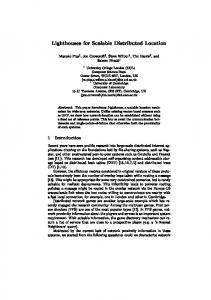
Figure 1: Example of a Mxed System Implementation must execute and the cycle-per-instruction (CPI) metric of the processor. In general, application-specific hardware implementations tend to be faster since the underlying hardware is tailored and optimized for the specific set of tasks. However in absence of stringent performance constraints, for a given behavioral description of an ASK machine, some parts (subroutines) of it may be well suited to a commonly available re-programmable processor (like 6502, 68HC11, 805 1, 8096 etc) while others may take too long to execute. For instance, most general purpose CPU’s deal with byte operands whereas many ASIC controllers contain bit oriented operations resulting in unnecessary overheads when implemented entirely in software. However, the software implementations do provide the ease and flexibility of reprogramming for the possible price of loss of performance. Example 1.1.
’
To be specific, consider design of a data encryption/protocol controller chip, such as DES (Data Encryption Standard) used by commercial banks or AES (Audio Engineering Society) protocol used for communication between digital audio devices and computers. In Figure 1, the DES transmitter takes data from memory using a DMA controller, assembles the frame for transmission, it encrypts the data after it receives the key and transmits the encrypted data. Encryption protocol requires that the encrypted data be transmitted within a certain time duration of receiving the encryption key. In the DES protocol, a 56-bit encryption key is used to transform 64 bits of ‘plaintext’. Software implementations of the encryption algorithm shown in Figure 2 vary from 300 to 3000 instructions depending on the level of bit-oriented operations supported. The hardware implementation on the other hand can be implemented to work in 16 cycles times of most digital systems. It is possible to implement the DES controller in Figure 1 either as a program on a general purpose re-programmable component or as dedicated ASIC chips [5]. However, as shown in Figure 2, most encryption/decryption is a long, iterative process of rotations, XOR operations, bit permutations and table lookups. Further, these protocols often use bit-reversal operations as a part of overall encoding strategy. A bit-permutation operation can be implemented easily in dedicated hardware while it may take too long to execute as a sequence of instructions on most processors. While implementing the complete protocol controller on dedicated hardware may be too expensive, an implementation which uses a re-programmable component may satisfy performance requirements and at the same time provide the ease and flexibility of reprogramming in software.
1. I
Motivations for hardware-software partitionikg
3
clear 64-bit output buffer for each bit i = 1 . . 48 of keyed buffer do { isolate bii i of the keyed . .buffer if (bit i = 1) set output buffer bit f(i) using map table, f 1 SOFTWARE: 300 TO 3000 INSTRUCTlONS
Permuted and Shifted 56-Kev. Buffer 9 10 11
. .
14 15 16
17
. .
21 . .
24
49 50 51 52 53 54 55 56
I
b b /I /
I1
byte 1
,/
/ 1
1
I
I
. byte 7
byte 2
/ I
I
1
,
byte 8
HARDWARE: MAXIMUM OF 16 CYCLES
Figure 2: DES Encryption Scheme
Example 1.2. While bit-wise shifting and xor operations lead to a slower software implementations, corresponding byte-wise implementations was considerably faster. Given extra memory for table-storage, the program implementations can be speeded-up even more using table-lookup methods. Such implementations are often competitive with corresponding hardware implementations. Consider a l&bit CRC-CCITT computation using polynomial z l6 + xl2 + x5 + 1 below. With the addition of every byte of data, the new CRC is clearly is a function of &bits of old CRC and the new byte of data. This function is precomputed and stored in an 256-entry table. Thus, a byte-wise implementation using two 256-byte tables, as described by the following pseudo-code, when coded in assembly can achieve 16-bit CRC computation in 7 instructions per byte. typedef byte char; byte Table_low[256], Table_high[256]; byte Temp, data, CRC-low, CRC-high; Temp = data xor CRC-low; CRC-low = Table-low[TempJ xor CRC-high; CRC-high = Table-high[Temp];
The actual latency of computation is a strongly dependent on the instruction-set architecture (ISA) of the target processor. The best implementation of the above pseudo-code on an Intel 8086 processor computes 16-bit CRCs in 9 instructions, a Motorola 68K implementation in 11 instructions and a RISC-based implementation in 14 instructions. 0
4
I
INYRODUCT7ON
1.2 The problem of system synthesis The problem of mixed system synthesis is complex, and todate there are no available CAD tools to support it. This report addresses the hardware-software codesign issue by formulating it as a system partitioning problem into application-specific and re-programmable components. As explained in Section 4, we can also view it as an extension of high-level synthesis techniques to systems with generic re-programmable resources. Nevertheless, the overall problem is much more complex and it involves, among others, solving the following subproblems: 1. Modeling the system functionality and performance constraints. System modeling refers to the speci’cution problem of capturing important aspects of system functionality and constraints to facilitate design implementation and evaluation. Most hardware description languages attempt to describe a system functionality as a set of computations performed by a computing element and as interactions among computing elements. Among the important issues relevant to mixed system designs are: 0 explicit or implicit concurrency specification --_ l communication model used: shared memory versus message-passing based l
control flow specification or scheduling information
There is a relationship between concurrency specification and the natural partitions in the system descriptions. Typically, languages that contain explicit partitioning via control flow breaks, find it difficult to specify concurrency explicitly. Concurrency information is then obtained by performing dependency analysis whose complexity depends on the communication model used. We consider the relevant modeling issues in Section 3. 2. Choosing granularity of the hardware-software partition. The system functionality can be partitioned either at the functional abstraction level where a certain set of high-level operations is partitioned or at the process communication level where a system model composed of interacting process models is mapped onto either hardware or software at the process description level. The former attempts fine grain partitioning while the latter attempts a high-level library binding through coarse-grain partitioning. 3. Determination of feasible partitions into application-specific and re-programmable components. The so-called problem of hardware-sofhuare partitioning. This delineation is influenced by issues such as analog interfaces that require a specialized hardware interfaces. However, for operations that can be implemented either in hardware or in software, the problem requires a careful analysis of flow of data and control in the system model. 4. Specification and synthesis of the hardware-software interface. 5. Implementation of software routines to provide real-time response to concurrently executing hardware modules.
.
1.3 Applications
5
6. Synchronization mechanisms for software routines and synchronization between hardware and software portions of the system. This report attempts to outline major issues and suggests approaches to solving them. This report is organised as follows. In Section 2.1 we present a description of different system architectures based on types of hardware, software components used. We then describe features and limitations of the system architecture that is target of current approach towards system synthesis. Section 3 describes the modeling of system functionality. In particular, we describe how the input to our synthesis system is described in a hardware description language and its model based on flow graphs. Section 4 defines the problem of system partitioning. We discuss issues relating to performance characterization of hardware and software components and partitioning cost metrices based on which a partitioning algorithm is presented. Sections 5 and 6 present problems and solutions in implementation of hardware and software components, respectively. We introduce the notion of threads as a linearized set of operations. The software component is composed a set of concurrent and hierarchical threads. Section 7 discusses issues in system synchronization, how synchronization is achieved between heterogeneous components --. of system design. In section 8 we present design network coprocessor and summarize the results of hardware, software tradeoffs. Section 9 presents a summary of the main issues in system synthesis. 1.3 Applications Among the potential applications of the techniques presented in this report are: 1. Design of cost-effective systems: ‘Ihe overall cost of a system implementation can be reduced by the ability to use already available general purpose re-programmable components while reducing the number of application-specific components.
a
2. Rapid prototyping of complex system designs - a complete hardware prototype of a complex system is often too big to be implemented except in a semi-custom implementation. With the identification of time critical hardware section, the total amount of hardware to be synthesized may be reduced significantly, thus making it feasible for rapid prototyping. A feasible partition that shifts the non performance-critical tasks to software programs can be used to quickly evaluate the design. 3. Speedup of hardware emulation software - During their development phase, many system designs are often modeled and emulated in software for test and debugging purposes. Such an emulation can be assisted by dedicated hardware components which provides a speedup on the emulation time. Rapid prototyping and hardware emulation are two opposite ends of the system synthesis objective. Rapid prototyping attempts to minimize the application-specific component to reduce design time whereas hardware emulation attempts to maximize the application-specific component to realize maximum speedUP*
6
2
SYS7EM ARCHmCTLRES BASED ON HARDWARE-SOFTWARE COMPOAEl System Specificatitm
System ParWoning .
Inkwfacw Generation
Assembly Code
ASIC and Interface Netlist
Mixed System implementation
Figure 3: System Synthesis Procedure
I
Figure 3 shows organization of the CAD design system used for synthesis of mixed system designs. The input to our synthesis system is an algorithmic description of system functionality described in a hardware description language (HDL). The HDL description is compiled into a system graph model based on data-flow graphs described in Section 3. ‘Ihe system graph model is subject to system partitioning and hardware and software generation schemes as described in sections 4 through 6. Section 7 discusses mechanisms for synchronization between hardware and software. The resulting mixed system design consists of an assembly code for the software component, and a gate-level description of the hardware and hardware-software interface. ‘Ihis heterogenous description can be simulated by a program Poseidon that is described elsewhere [6].
2 System Architectures Based on Hardware-Software Components In colloquial terms most digital systems can be classified as being either reprogrummable or embedded. Reprogrammable digital systems contain some form of storage that can be altered (reprogrammed) by the user under software control. On the other hand, the embedded systems are usually hardwired for certain
7
Degree of Reprogrammability
ii is! g Reprogrammable 2 Micro-prog
0
0
MicroProgram
:
ML prOgriUll
BITGLICED CONTROLLERS
MAINFRAMES VLIW MACHINES MICROCONTROLLERS ,
4
HL Program
MLXED
CONTROLLERS Custom Hardware
Synthesized Hardware
Programmable U’W (F-V
HARDWARE COMPONENT Figure 4: System Classification Based on HUYSW Components
a
specific tasks which can not be altered without changing the underlying hardware. Most reprogrammable digital systems contain one (or more) general-purpose microprocessor and structured memory components. Since embedded systems are optimized for certain specific tasks, the degree of ‘reprogrammability’ varies from none to changing parameters of some existing sequential control. An embedded system may have a dedicated controller (a sequencer) or a microcontroller programmed to sequence operations. Most of these systems contain storage (program or data) which is relatively small and can not be easily altered. Microcontrollers are essentially general purpose microprocessors with on-board memory for program and data storage. The ability to reprogram a digital system is related to the versatility of primitive operations, or the instruction-set of the microprocessor or microcomputer used in the system. In our terminology we refer to a microprocessor or a microcontroller as a reprogrammable component or simply as a processor. The specific set of instructions needed for a particular application to be executed by the reprogrammable component is referred to as the software component. Thus, in broad terms, a digital system can be thought of consisting of two components: sofrware as a program in an on-board RAM or ROM and hardware as the underlying interconnection of special-purpose blocks. Based on this distinction, Figure 4 shows compositions of some familiar systems. The hardware component in a system design may be customdesigned as in most general purpose machines, or program-generated (programmed), or programmable as in programmable gate array designs. The software component of a system may consist of microcoded routines, or machine-level programs used in embedded control systems or high-level programming used in special-purpose machines. It is important to note that some system designs use microcoding simply as a technique for implementation of hardware control. For example, general purpose microprocessors
2 SYSlEM ARCHmCTUES BASED ON HARDWARE-SOFTRGIRE COMPOAENlS
8
MICRO- 0 7 0 c)
ASK
PROCESSOR -
- ASK
Figure 5: Target System Architecture use microcoding simply as a design technique. This is different from the software necessary to achieve system functionality as in microprogramming of functional algorithms in case of mainframe machines. Conventionally, machine-level and high-level programs manipulate user data-structures while microprograms manipulate hardware resources. In case of mixed controller designs proposed in this paper, however, we use machine-level programs to perform both activities. The objective of this research is design of mixed controllers shown in Figure 4. These systems use a reprogrammable compoent to achieve part of the system functionality which may be time-constrained as in the case of embedded systems. 2.1 Target System Architecture We choose a target architecture that contains the essential elements of hardware-software systems. In a Figure 5, the target architecture consists of a general-purpose processor assisted by application-specific hardware components. The following lists the relevant assumptions relating to the target architecture. 0 We restrict ourselves to use of a single re-progrumrnuble component because presence of multiple re-programmable components requires additional software synchronization and memory protection considerations to facilitate safe multiprocessing. Multiprocessor implementations also increase the system cost due to requirements for additional system bus bandwidth to facilitate inter-processor communications. We make this simplifying assumption in order to make the synthesis tasks manageable. l
The memory used for program and data-storage may be on-board the processor. However, the interface buffer memory needs to be accessible to the hardware modules directly. Because of the complexities associated with modeling hierarchical memory design, so far we considered the case where all memory accesses are to a single level memory, i.e., outside the re-programmable
9 component. The hardware modules are connected to the system address and data busses. Thus all the communication between the processor and different hardware modules takes place over a shared medium. l
The re-programmable component is always the bus master. Almost all re-programmable components come with facilities for bus control. On the other hand, inclusion of such functionality on the application-specific component would greatly increase the total hardware cost.
l
All the communication between the re-programmable component and the ASIC components is done over named channels whose width (i.e. number of bits) is same as the corresponding port widths used by read and write instructions in the software component. The physical communication takes place over a shared bus. The problem of encoding and sharing multiple virtual channels over a physical bus is a subject of continuing research at Stanford [7].
l
The re-programmable component contains a ‘sufficient’ number of maskable interrupt input signals. For purposes of simplicity, we assume that these interrupts are unvectored and there exists a predefined destir@on address associated with each interrupt signal.
l
The application-specific components have a well-defined RESET state that is achieved through system initialization sequence.
It is important to note that the final system implementation may or may not be a single-chip system design depending on availability of the re-programmable component either as a macro-cell or as a separate chip. Further, the approach outlined in this report can also be used for alternative target architectures.
3
Specification and Modeling of Hardware-Software Systems
Currently most behavioral system specifications are derived from the corresponding algorithmic descriptions of the system functionality. The algorithmic descriptions are usually described in a procedural language like C or Pascal. Consequently, the hardware behavioral descriptions tend to use a procedural - language like VHDL, Verilog etc. However, when describing hardware in a procedural language (that is, as a program), one is often faced with the difficulty of representing an essentially concurrently-executing set of operations in a linear code The linear-code representation inherently assumes existence of a single thread of control and static data storage. However, hardware execution is usually multi-threaded and is driven by availability of appropriate data. In contrast to instruction-driven single-threaded linear-code representation, data-flow graphs provide a dutu-driven representation that can model multiple-threads of execution (Figure 6). Therefore, the hardware for embedded controllers and non-recursive DSP algorithms is more appropriately represented by data-flow (DF) graphs instead of linear code used for algorithmic description. To avoid this dichotomy of behavioral representation, most high-level synthesis algorithms operate on an intermediate form that accurately reflects the concurrent nature of hardware. Most hardware intermediate forms used for high-level synthesis tend to be similar to data-flow graphs [S] [9] [lo] [ll]. Generally, any sequence of machine instructions can be represented by a machine-level data-flow graph. Indeed the expression-evaluation trees generated by compilers (before the code-generation stage)
10
3
SPECIHC-AlTON AlK?I MODELING OF HARDWARE-SOFTWARE SYSEMS
scheduling and code gmefathn
r
L1lb.W
l
htnmtion mwn Singlo Thrwd of Executitm L/near, Static dbt8 rturo
Figure 6: Linear Code versus Data-How Graph Representations are a form of data-flow graphs. However, these data-flow graphs consisting of operations described at the level of machine instructions decrease the specification granularity significantly to make them useful for system partitioning in to hardware and software components. Therefore, data-flow graphs in our context are described using operations available at the language specification level. These have also been referred to as macro-data flow graphs elsewhere [ 121. From data-flow representations we can generate an equivalent sequence of instructions by scheduling various operation vertices in the data-flow graph. Operation scheduling techniques are important even in case of a single thread of execution where static memory requirements are affected by scheduling even though all schedules result in same overall latency (see Section 4.2) . Latency optimality in scheduling is realized by exploiting parallelism in instruction stream which requires multiple execution threads. We consider the algorithms for evaluating data-flow graphs and their equivalent linear-code representations in section 4.2. 3.1 System specification using HardwareC a
We specify system functionality in an hardware description language called, HurdwareC [ 131. HardwareC follows much of the syntax and semantics of the programming language, C with modifications necessary for correct and unambiguous hardware modeling. Like C, the primitive operation in HurdwureC consists of an assignment operation with a procedural call being the means of abstraction of sub-specifications. Procedural calls correspond to modular specification of different components of the hardware. No recursive calls of any form are allowed. A HardwareC specification consists of blocks of statements which are identified by enclosing parentheses. The blocks are structured, thus no two blocks are overlapped partially. That is, given any two blocks, they are either disjoint or one is contained by the other block. Like C, no nested procedure declarations are allowed. Therefore, any variable that is non-local to any procedure is non-local to all procedures. Local variables are scoped ZexicuUy with the most-closed nested rule for structured blocks. A process in HardwareC executes concurrently with other processes in the system specification. A process restarts itself on completion of the last operation in the process body. Thus there exists an
.
3.1
System specification using HardwareC
11
implied outer-most loop that contains the body of the process model. In other languages, this loop can be specified by an explicit outer loop statement. Operations within a process body need not be executed sequentially (as is the case in a process specification in VHDL, for example). A process body can be specified with varying degrees of parallelism such as.parallel (< >), data-parallel (0) or sequential ([I). In addition, HardwareC allows specification of declarative model calls as blocks that describe physical connections and structuraI relationships between called models. For hardware modeling purposes, both timing and resources constraints are allowed in the input specifications. Timing constraints are specified as min/max delay attributes between labeled statements where as resource constraints are specified as user-specified bindings of process and procedure calls to specific hardware model instances. Example 3.1 describes a simple process specification in HurdwareC. Example 3.1.
Example of a simple HurdwureC process process simple (a, b, cl in port a[8], b[8] ; out port cl81 ; _-boolean
xi81, ~181, 2[81 ;
< x = read(a); y = read(b); 2 = fun(x , y); write c = 2;
This process performs two synchronous read operations in the same cycle, followed by a function evaluation and a write operation. Note that specification of explicit parallelism by () delimiters is redundant here since there exists an implicit parallelism between the two read operations, thus a data-parallel grouping (0) would yield the same execution results. 0 There is no explicit delay associated with individual assignment statements (except in case of explicit
a register/port load operations as mentioned later). An assignment may take zero or non-zero delay time. However, multiple assignments to same variable can either be interpreted as (a) last assignment or (b) an assignment after some delay. Resolution of which policy (a) or (b) to be used is performed by a reference stack [ 141. Reference stack performs variable propagation by instantiating values of the variables in the right-hand side of the assignments. In case of identified storage elements (b) is adopted where ‘some delay’ corresponds to delay of ‘at least’ one cycle time. In addition, this policy can also be enforced on some assignments by an explicit ‘load’ prefix that assigns a delay of precisely one cycle time to the respective assignment operation. 3.1.1 Memory and Communication HardwareC allows specification of shared memory within a process model. All the communication
within a process model is based on the shared memory specified within the model, because it is relatively straight-forward to ensure ordering of operations within a given process model to ensure integrity of
.
12
3
SPECIEICATTON AND MODELING OF HARDWARE-SOFTWARE SYSTEMS
memory shared between operations in the model. However, consistency of memory shared across concurrently executing models must be ensured by the models themselves. HardwareC allows specification of blocking inter-model communications based on message-passing operations. As with the shared memory variables, the only data-types available for channel is a fixed-width bit-vector. Integers are coded .. using 2’s complement representation. Use of message-passing operations simplifies the specification of inter-model communications. It should be noted, however, that it is easy to implement a message-passing communication using memory shared between respective models (the converse is not true, however). Indeed, during system partitioning, reductions in communication overheads are realized by simplifying the inter-model communication as discussion in later sections. 3.1.2 Nondeterminism in System Specifications Non-determinism in our system models is caused either by external synchronization operations or by internal data-dependent delay operations, like conditionals and data-dependent loops. External synchronization operations are related to blocking communication operations, whereas operations likes datadependent loops present variable and unknown execution delays. Example 3.2 below shows a HurdwareC process description containing 3 unbounded/unknown delay operations: message-passing receive operation, conditional and loop. Example 3.2.
Example of a HurdwareC process with unbounded delay operations process example (a, b, c) in port a[81 ; in channel b[8] ; out port c ; boolean x181, y[8 I, 2181 ; x = read(a); y = receive(b); if (x > y) Z = x - y ; else z=x*y; while (z >= 0) ( write c = y z=z-1;
read refers to a synchronous port read operation that is executed unconditionally as a value assignment operation from the wire or register associated with the port a. receive is a message-passing based read operation where the channel b carries additional request and acknowledge control signals that facilitate a blocking read operation on based on availability of data on channel b. 0
3.2 System Model Broadly speaking, there are two major ways of modeling and analyzing the system behavior:
13
3.2 System Model
process-based modeling where logical and temporal properties of processes and their constituent events define the behavior of a system, and axiomatic techniques, similar to theorem-proving in proof systems, are applied to verify correctness of system transformations [ 15 1. Relevant logical properties of the system behavior are expressed by assertions about liveness and safety. Each liveness property indicates that the assertion (about state of the system) will eventually hold. Each safety property states that the assertion (on the system state) ~31 always be true. Most common method to specify and verify such assertions is by adding time variables to the computation model [ 161 [ 171. Common examples of this approach are proof-systems for CSP programs [ 181, distributed programs [ 191. graph-based modeling which uses techniques from graph theory to build the system model. The main difference with the process-based modeling is in explicit expression of dependencies between processes and constituent operations. We model system behavior using a graph representation based on flow graphs [20]. As described later in this section, timing and resource constraints are represented on graphs compatible with the operation graph models. -_ Definition 3.1 A system model, M, is represented by a 3-tuple consisting of operation graph Pr, timing constraint , 7, and resource constraint, R.
The operation graph models capture system functionality as a set of control-data-flow graphs. ‘Ilming constraints are specified using compatible weighted graph models. Resource constraints are used to specify bounds on types and number of data-path resources available for synthesis of M into hardware as well as the amount of static storage available for synthesis of M into software. Hardware resource constraints are important for hardware synthesis and are briefly mentioned in Section 5. Definition 3.2 An operation graph model, #, consists of a set of acyclic sequencing graph models: where a sequencing graph model, Gi, represents body of an iterative construct in the hardware description language model.
The iterative constructs are of two types: l l
Counting loops have an explicit or an implicit repeat count, T. Non-counting loops wait on some external conditions on a wire or a channel. For example, a HardwareC statement like
while(wirename); is semantically equivalent to wait ( !wirename) ;. These loops model some asynchronous event in the behavior model and are required for correct modeling of reactive hardware behavior. The corresponding hardware for such loops is implemented by means of asynchronous set/reset inputs to the storage elements. In software, however, such operations can be implemented either as interrupts to on-going computation or as polled operations.
3 SPECZTCATTON Am MODEL~G OF HARDWARE-SOFTWARE SYSZMS
14
All sequencing graph models are assumed to model counting loop operations with a finite or infinite repeat count. Non-counting loop operations are modeled as individual wait operations. We make further distinctions between characteristics of counting loop constructs when considering issues in performance characterization of the software component. A sequencing graph model, G, that models a process specification in HardwareC is a model with Infinite repeat count., that is, on completion of its last operation (sink), it restarts itself unconditionally. Among the sequencing graph model of an operation graph model, 6, there are two kinds of hierarchies induced: l
l
structural hierarchy denoted by relation, S, that denotes structural relationship between any two sequencing graph models, calling hierarchy G* of a sequencing graph model, G, denotes the set of sequencing graph models that are on the control-flow hierarchy of G, that is, models that are called or used by G.
An operation graph model may consist of structural connection of one or more than one sequencing graph models, each of which contains a called hierarchy. A sequencing graph model that is common to two calling hierarchies is considered a shared model or a shared resource. Definition 3.3 A sequencing graph model is a polar acyclic graph G = (V, E, S, x, S) where V = {BOA,... , v~) represent operations with vo and VN being the source and sink operations respectively. The edge set, E = ((vi, vj )) represents dependencies between operation vertices. An integer weight S(vi), \d vi E V represents execution delay of operation associated with vertex, v;. Function, x : E I+ 2 defines condition index of a given edge. case of edges incident from a condition vertex or incident on a join vertex, these a condition index refers to case value associated with the evaluated condition. S defines the storage common to operations in the graph model G.
In
I
For sake of simplicity, a sequencing graph model, G, is often expressed as G = (V, E). An edge, (vi 7 vj) E E(G) induces a precedence relationship between vertices v; and vj and it is also indicated by Vi > vj. Relation >* indicates transitive closure of the precedence relation. The transitive closure of a sequencing graph model, G, under precedence relation is denoted by G? Note that the sequencing model defined here are similar to the the SIF model defined in [ 141. There are, however, some differences in representation of conditional and wait operations. The sequencing graph model captures the operation concurrency and data-dependent delay operations. Overall, the sequencing graph model consists of concurrent data-flow sections which are ordered by control flow. The graph edges represent dependencies while branches indicate parallelism between operations. The data-flow sections preserve the parallelism while control constructs like conditionals and loops obviate the need for a separate description of the system control flow. The control operations like loops are specified as separate subgraphs by means of hierarchy. The computational semantics of the sequencing graph model is as follows: an operation in the data-flow graph is enabled for executions once all the input data are available. We maintain the strict FXFO order of operations during successive invocations of the graph model by imposing the additional constraint that a source vertex is reinvokes only after the corresponding sink vertex has been executed. This requirement avoids need for conventional
3.2 System Model
15
token-matching schemes needed for execution of pure data-flow graphs [21]. Figure 7 shows an example of the graph model corresponding to process simple described in Example 3.2.
w0 ._ 0 fd d 1 \0
/ bI
d
1
fun 2
. 0
nop 0
Sink
s = Ix Y, zl
Figure 7: Example of a sequencing graph model Remark 3.1 Storage, S, is decfined for correct behavioral interpretation of the graph model, G. S is independent of cycle-time of the clock used to implement the corresponding synchronous circuitry and does not include storage spec@c to structural implementation of G (for example, control latches). Further S, need not be the minimum storage requiredfor correct behavioral interpretation of a sequencing graph model.
An operation vertex is classified as a simple or complex vertex depending on the operation performed by the vertex. Simple vertices consist of a single operation whereas complex vertices consists of a set of operations that are represented by a called sequencing graph model. Thus complex vertices induce hierarchical relationships between sequencing graph models. A call vertex enables execution of the sequencing graph corresponding to the procedure call. A loop vertex iterates over the graph body of the loop until its exit condition is satisfied. Table 1 lists operation vertices used for describing the sequencing graph models. Remark 3.2 The sequencing graph is acyclic because the HardwareC descriptions are required to be structured and looping constructs are represented as separate graphs.
Data-dependent and synchronization operations introduce uncertainty over the precise delay and order of operations in the system model and thus make its execution non-deterministic [22]. We refer to a vertex with data-dependent delay as a point of non-determinism in the system graph model.
16
3
SPECLKK’Al7ON AND MODELING OF WARDWARE-SOFTl+HRE SYS7EM.S 0Pe
Description
Operation
no-op load .. cond join wait op-logic op-arithmetic op-relational op-io Complex call loop block
Simple
No operation Load register Conditional fork Conditional join Wait on a signal Logical operations Arithmetic operations Relational operations I/o operations Procedural call Iteration Declarative block
Table 1: Sequencing graph operation vertices
Definition 3.4 An operation vertex in G with an unbounded execution &lay is known as an anchor vertex. A vertex representing wait operation is example of an anchor vertex. The execution delay, 6(v) of an anchor vertex may not be known statically and may take any nonnegative integer value from 0 to 00. By definition, source vertex, VO, of a sequencing graph is considered an anchor vertex. Definition 3.5 A sequencing graph delay function, d, returns a non-negative delay of a graph model, G following a bottom-up computation as follows: I
1. Delay of a non-anchor vertex is the execution delay of the operation, d(v;) = 6(v;), 2. Delay of an anchor vertex is set to zero, 3. Delay of a sequencing graph model, G, is the delay of the longest path in G,
d(G) = maxd(poN) =
c ui E longestgath(G)
4Vi)
where a path,pij, in G consists of an ordered set of vertices in V(G), p;j = (v;, v;+l, . . . , vj>. 4. Delay of a complex vertex is set to zero, that is,
d(vlocJ = d(vcau) = +4hck) = 0 5. Delay of a conditional vertex is maximum of delay over each of its branches. A conditional branch is defined by a directed path from the condition vertex to the corresponding join vertex.
.
3.2 System Model
17
Definition 3.6 A sequencing graph latency function, X, returns a non-negative latency of a graph model, G following a bottom-up computation as follows: 1. Latency of a vertex is the execution delay of the operation represented by vertex 2. Latency of a sequencing graph model is execution delay of the sequencing graph model, that is, the time period from execution of its source vertex to the execution of its sink vertex 3. Latency of complex vertices is the latency of the corresponding called sequencing graph models, that is,
+block)
=
A(Gblock)
where ~1 is the repeat-count of the loop operation vlOOP.
Note that latency of a sequencing graph is a function of operation scheduling. On the other hand, the delay function represents the longest path delay of sequencing graph. 3.2.1 Communication For all operations with in in a graph model, G = (V, E, 6, S) all the communication is based on shared storage, S. Inter-model communications are represented by I/O operation vertices which, on execution, may alter the model storage, S. An I/O operation vertex may encapsulate a sequence of operations which is referred as a communication protocol. A communication protocol may be blocking or non-blocking. A non-blocking protocol may also be finitely buDred. A blocking communication protocol is is expressed as a sequence of simpler operations on ports and additional control signal to implement the necessary handshake. For example, to implement a blocking read operation on a channel ‘c’additional control signals ‘cxq' and ‘c-ak' would be needed as shown in the Example below. Example 3.3. bread(c)
A blocking read operation. =>
[ write c-rq = 1; wait(c-ak); < read(c); write c-rq = 0; >
cl
While it is easy to connect two blocking or two non-blocking read-write operations, connection of two disjoint read/write operations on a channel requires handling of special cases. For example, consider a connection between blocking read and non-blocking write operation below. Example 3.4.
Blocking/Non-blocking channel connections.
3 SPECITK’A7TON AND MODELING OF HARDWARE-SOFTUHRE SYSTEMS
18
PlodlJCW
Consumer
Blocking read and non-blocking write Blocking read
Non-blocking write
[
[
write c-rq = 1; wait(c-ak); < read(c); write c-rq = 0; >
write c-rq = 1; < write c = value; write c-rq = 0; > I
Blocking write and non-blocking read Blocking write
Non-blocking read
[
[
write c-rq = 1; < read(c); write c-rq = 0; z
write c-rq = 1; wait(c-ak); < write c = value; write c-rq = 0; >
1
A non-blocking/non-blocking read/write connection results in one cycle read and write operations. However, a blocking/non-blocking connection requires two clock cycles for the non-blocking operation. 0
A buffered communication is facilitated by a finite-depth interface buffer with corresponding read and write pointers. The communication protocol consists of I/O operation as well as manipulation of the read, write pointers as shown by the example below. Example 3.5.
Buffered communication protocol. Producer
Consumer
writegtr C
1 read (buff[readqtr]); read_ptr++ modulo N;
I write buff[write_ptr] = value; writegtr+t modulo N;
Under normal operation, reattptr # write,ptr. Violation of this condition indicates either a buffer is full or empty depending on whether the increment of writ e-ptr causes violation or the increment of rea&ptr causes the violation. 0
3.3
SpeCfication of 7Rning Constraints
19
Figure 8: 77~ Constraint Graph Model 3.3 Specification of Timing Constraints liming constraints are of two types: (a) minimum/maximum timing separation between pairs of operations and (b) system input-output rate constraints. ‘Ikning constraints between operations are indicated by tagging the corresponding operations. The input(output) rate constraints refer to the rates at which the data is required to be consumed (produced). The rate constraints refer to min/max time constraints on multiple executions of the same input or output operation. Let us first consider the timing constraints of the first type, that is, the min/max timing constraints. Min/max timing constraints between operations are specified by tagging the corresponding assignment operations in the HurdwareC specifications. Example 3.6 shows an example of a min/max timing constraint. Example 3.6.
Specification of midmax timing constraints by statement tagging process simple (a, b, cl in port a[8], b[8] ; out port c[S] ; boolean x[8], y[8], z[8] ; tag A, B;
< A: x = read(a); y = read(b); z = fun(x , y); B: write c = z; constraint
maxtime
from A to B = 3 cycles;
0
These timing constraints are abstracted in a constraint graph model [14] shown in Figure 8. In the constraint graph model vertices represent operations and edges indicate timing constraints between
20
3 SPECIEK’A77ON An-I) MODELJNG OF HARDWARE-SOFTWXRE SYS7lZMS
vertices. The edges are Weighted by the timing constraint value. A positive value implies a minimum timing constraint, a negative value implies a maximum timing constraint. Let T(vi) represent start time of operation v;. A minimum timing constraint, Zij 2 0 from operation vertex v; to Vj is defined by the following relation between the start times of the respective vertices:
Similarly a muximum timing constraint, Uij 2 0 from vi to vj is defined by the following inequality: T(vj) 5
Uij
T(v~) +
Definition 3.7 The timing constraint graph model, GTO is defined as GT~ = (V, E, 0) where the set of edges consists of forward and backward edges, E = Ej U Eb and W;j E n defines the weights on edges such that T(vi) + Oij < T(vj).
3.4 Data Rate Constraints Each execution of an input(output) operation consumes(produces) a sample of data. An input/output data interval is defined in terms of cycles/sample as the interval between successive input/output operations. Corresponding data rates are defined by inverse of the data interval. Input/output data rates are a function of time. A minimum data rate constraint, pm, on an input/output operation defines the lower bound on the interval between any successive executions of the corresponding operation. Similarly, a maximum data rate constraint, PM, on an I/O operation defines the upper bound on the time interval between successive executions of the operation. Thus, the rate constraints refer to time constraints on multiple executions of the same input or output operation. These constraints can be expressed as min/max timing constraints on unrolled constraint graph models. As an example, constraint graph model GT~ shown in Figure 9 consists of two sequential executions of the sequencing graph model G. The rate constraint on consecutive read operations is shown as a maximum timing constraint between two read operations in GT1. For an I/O operation v E V(G), a data-rate constraint of PM samples/cycle can be translated into a constraint on latency of G. Graph G either models a process or body of a loop operation. If G models a process then execution of G restarts itself on completion. Since polarity of G guarantees that there is one execution of v for every execution of G. Therefore, latency, A(G) 5 & cycles. If G models body of a loop operation vi E V( G’) then A(G’) = X(vl) + d’ = 1-1 A(G) + d’ l
where d’(2 0) is the difference in latencies of G’and vi. Thus a constraint on A(G) can be translated into a constraint on latency of the corresponding process graph model, G’, if the loop repeat count, rl, can be constrained. In case of nested loop operations, rate constraints are indexed by corresponding loop operations. ‘Ihe loops are indexed by increasing integer numbers. The inner-most loop is indexed 0. In the Example 3.7 below there are two rate constraints on the read operation with respect to the two while statements.
21
3.4 Data Rate Constraints
Figure 9: SpecilLication of rate constraint as a midmax timihg constraint Example 3.7.
Specification of rate constraints in presence of nested loop operations. process example (frameEN, bitEN, bit, word) in port frameEN, bitEN, bit; out pert word(81; boolean store[8], temp; tag A; while (frameEN) while (bitEN) A:
temp = read(bit); store[7:0] = store[6:0] @ temp; write word = store; attribute 'constraint maxrate 0 of A = attribute 'constraint maxrate 1 of A =
1 cycles/sample'; 10 cycles/sample';
QO
0mg
Ql OP Q
8
1
Q
Q2
1
-mg 0
0 *
l( (32)
v) ; Vu E pred(u) count = count - 6(v>il) ; storage = mar(count, storage) ; --. 1 return storage 1 0
Lineaxization using Topological Sorting Input : data-flow graph model, G(V,E) Output: a list of topologically ordered vertices topologicallymder(G) ( Q= stack = {} ; VuO’(G) U = white ; source-vertex(G) = gray ; push (source-vertex(G)) ; . while stack # {} { Vu E Aaj(Top (stack)) { if v = white { u = gray ; push(v) } 1 Q=Q + pop( stack) ) return
Q
}
4.3 Partitioning Feasibility
S = ( a, b, c, d, 8, f, g)
27
min static storage, min(lSI) = 3
Figure 10: Detmhation of minimum static storage for sibgle execution thread 4.3 Partitioning Feasibility
.
A system partition into-an application-specific and a re-programmable component is considered feasible when it implements the original specifications and it satisfies the performance and interface constraints. We assume that the hardware and software compilation, done using standard tools, preserves the functionality. We, therefore, concentrate on constraints. In particular, timing constraints are of special interest. As noted earlier, timing constraints are of two types: those related to m.in/max time separation between different operations and rate constraints on I/O operations. We assume that the operations subject to a min/max timing constraint belong to the same process model. A timing constraint between operation belonging to two different processes is equivalent to a synchronization constraint between the processes and it can be specified by a blocking inter-process communication in functional specification of the processes. Rate constraints are translated as constraints on latencies of affected sequencing graph models and thus verified by comparing actual hardware and software latencies against imposed bounds. Satisfiability of min/max timing constraints is checked by analyzing the corresponding constraint graph models. For graphs with no unbounded delay operations, constraint satisfiability is related to absence of any positive cycles in the constraint graph model. However, in presence of unbounded delay operations, some constraints may be ill-posed [26], that is, constraints that can not satisfied for some possible values of delays of unbounded delay operations. Note that a minimum timing constraint is never ill-posed. For an illsposed maximum timing constraint between vertices vi and Vj there are two cases: 1. operations Vi and vj are transitively related, i.e., Vi >* Vj, 2. conversely, operations are concurrent, that is, l(Vi >* Vj) & l(Vj >* Vi). In the first case, there exists a path, pij, that contains an unbounded delay operation. The unbounded delay operation may be an external wait operation or an internal loop operation. For the software implementation of the graph model, a wait operation is made deterministic by performing a context switch to a other operations. Thus, satisfaction of the timing constraint by the software component can be verified by assigning appropriate context switch delay (as mentioned in the previous section) to the wait operation. In presence of general unconstrained data-dependent loop operations, determination of satisfiability of
28
4 7IHE PROBLEM OF HARDWARESOFTWARE PARlT7TONZNG
timing constraint is undecidable. However, under special conditions constrained loop operations can be made deterministic by choosing an appropriate policy of loop computation (as shown in the following sections). In the second case, where the constrained operations are concurrent, the constraint can be made well-posed by selective serializations between the two paths of computation. As mentioned earlier, when partitioning system model into hardware and software components the data rates may not be uniform across models. The discrepancy in data-rates is caused by the fact that the application-specific hardware and re-programmable components may be operated off different clocks and the system execution model supports multi-rate executions that makes it possible to produce data at a rate faster than it can be consumed by the software component when using a using a finite sized buffer. In presence of multi-rate data transfers, feasibility of hardware-software partition is determined by the fact that for all data transfers across a partition, the production and consumption data rates are compatible with a finite and size-constrained interface buffer. That is, for any data transfer across partition, data consumption rate is at least as high as the data production rate. The size of the actual buffer needed may then be determined by using the scheme proposed in [27]. In addition, since the target architecture as shown in Figure 5 contains a single system bus over which data transfer to and from the re-programmable component takes place: Therefore, the net effect of all data-transfers over this bus should not exceed the pre-specified system bus bandwidth. Available bus bandwidth is a function of bus/processor clock rate and memory latency. 4.4 Algorithms for System Partitioning The partition problem of hardware and software components requires first finding a feasible partition. Among data-rate feasible solutions, a cost jhnction of overall hardware size, program and data storage cost, bus bandwidth and synchronization overhead cost is used to determine the quality of a solution. We explore two approaches to obtain a partition of system model into hardware and software components. 4.5 System Partitioning based on system non-determinism a
We consider approaches to system partitioning in the order of increasing complexity of the system model. Let us first consider a system graph model with no unbounded delay operations and with single-rate execution model. We then look for a partition of a system model driven by satisfaction of the imposed timing constraints. Consider an algorithm that is summarized as follows: starting with an initial solution with all operations in hardware, we select operations for move into the software component based on a cost criterion of communication overheads. Movement of operations to software requires a serialization of operations in accordance with the partial order imposed by the system model. With this serialization and analysis of the corresponding assembly code for a given re-programmable processor, we derive delays through the software component. The movement of operations is then constrained by satisfaction of the imposed timing constraints. Such a partitioning algorithm would strive to achieve maximal number of operations in the software component. In presence of unbounded delay operations, we can still apply the algorithm described before. Note that unbounded delay operations can not be subject to any maximum timing constraints. Therefore, we
4.5 System Partitiolu’ng bas& on system non-determini~m
29
transfer all such operations into the software component and then identify deterministic delay operations for move into the software component such that all timing constraints are satisfied. However, in systems with multi-rate execution model, the datadependent delay operations makes it difficult to predict actual data-rates of production and consumption across partitions. Further, nondeterministic delays in the system model makes it difficult to statically schedule operations in any implementation of the system design. When considering a mixed implementation of the system design, it is possible to use dynamic scheduling of operations either or in both hardware and software components. Dynamic scheduling of operations in hardware or software requires both area and time overheads that may sometimes render a hardware-software co-design solution difficult or even infeasible. On the other hand, use of static scheduling requires a careful analysis of data-transfer rates across hardware and software portions in order to make sure that possible data-rates can indeed be supported by the interface implementation. Due to non-determinism in system models, the most general implementation of hardware and software components requires a control generation scheme that supports data-driven dynamic scheduling of various operations. Since the software component is implemented on a processor that physically supports only single thread of control, realization of concurrency in software entails both storage area and execution time overheads. On the other hand, in absence of any point of non-determinism from the software, all the operations in the software can be scheduled statically. However, such a software model may be too restrictive by requiring the control flow to be entirely in hardware. In our model of software implementation, we take an intermediate approach to scheduling of various operations as described below. First, we make following assumptions about the implementation model: l
l
The system has an application-specific hardware component that handles all external synchronization operations. (External non-determinism points). All the data dependent delay operations (internal non-determinism points) are implemented by software fragments running on re-programmable components.
The software component is thought to consist of a set of concurrently executing routines, called threads. - A thread consists of a linearly ordered set of operations. The serialization of the operations is imposed by the control flow in the corresponding graph model. Concurrent sets of operations are implemented as separate threads to preserve concurrency specified in the system graph model. All the threads begin with a point of non-determinism and as such these are scheduled dynamically. However, within each thread of-execution all operations are statically scheduled. As an example, data-dependent loops in software are implemented as a single thread with a data-dependent repeat count. In this way, we take an intermediate approach between dynamic and static scheduling of software operations. Instead of scheduling every operation dynamically, we create statically known deterministic threads of execution which are scheduled in a cycle-static manner depending on availability of data. Thus, an individual operation in software has a fixed schedule in its thread, however, the time and the number of times the thread may be invoked is data-driven. Therefore, for a given re-programmable processor, the latency,& of each thread is known statically. For a given data-input operation in a thread, i, with latency, Xi, the data consumption rate, pi is bounded as: e ma2 5 pi 5 k where ArnaZ refers to the latency of the longest thread. It is assumed that the latency includes any synchronization overhead that may be required to implement multiple threads
4 THE PROBLEM OF HARDWARE-SOFTWARE PARITTTOAING
30
Partirion Input: System graph model, G = ( V, E ) Output: Partitioned system graph model, V = V’U Vs .. partition(V): v = vduvn V” = V”* lJ V”t VH ={ vne, Vd} vs = { V”* } create software threads (Vna) compute data rates (processor) if not(feasible(VH, Vs)) exit fmin = WH, w
/* identify points of non-determinism */ /* external vs internal nondeterminism */ /$ the initial hardware component */ /$ the initial software component */ I$ create 1 Vni 1 routines */ /* No feasible solution exists */ r* initialize cost function */
repeat
foreach Vdi E Vd n VH
/* select a deterministic delay operation */ /* recursively move operations to SW */
mOVe(vdi)
until no improvement in cost function return(
Vjf , Vc) /* considers a vertex for move from V’to VS */
t?lOVe(vd i):
if feasible(VH - {vdi}, Vs + {vdi})
if f(VH - {Vdi), VS + {V”i}) < f&n VH = VH - ( Vdi ) VS = VS + { Vdi } fmin = f(VHrVS) update software threads update data rates (processor) foreach vdj E SUCC(vdi) t? VH
/* move this operation to
SW
*/
/* identify successor for move */
IIIOVe(vdj) return
of execution on a single-thread re-programmable processor. The lower bound on pi is obtained by implementing a software scheduling scheme that reschedules a repeating thread for execution at the end of every iteration. The system partitioning across hardware and software components is performed by decoupling the external and internal points of non-determinism in the system model. It is assumed that for all external points of non-determinism, the corresponding data-rates are externally specified. Thus, through this decoupling we are able to determine all the data-rates for all the inputs to the re-programmable component. The production data-rates of the re-programmable component are determined by the software synchronization scheme used. We consider the issue of software implementation in Section 6. From externally specified data rates we compute data rates for data flow edges in the system graph model. The vertex set, V, consists of two sets of vertices, V = {V d, Vn}, where Vd denotes the set
4.6 Partitioning based on decoupling of control and execution
31
of operations whose delay is bounded and known at compile time, and Vn refers to non-deterministic delay vertices. With a data-rate annotated system model as an input, we first isolate its points of nondeterminism, Vn, into two groups: VQ, those caused by external input/output operations, and Vni , those caused by internal data-dependent operations: The external points of nondeterminism, Vnc, are solely assigned to the hardware while the internal points of non-determinism, V W, are assigned solely to the software component. With this initial partition we determine the feasibility of data transfers across the partition. If this initial partition is not feasible, then the algorithm fails since no feasible partition exists under the proposed hardware-software interface and software implementation scheme. If the initial partition is feasible, then it is refined by migrating operations from hardware to software (i.e., moving vertices from V’to I+) in the search for a lower cost feasible partition. Associated with each internal point of non-determinism (e.g. data-dependent loop bodies) we create a program fragment or a thread of execution. Each thread of execution corresponds to a software routine by creating corresponding C code from HurdwareC description. For various threads of execution in the software component, we derive latency and static storage measures by analyzing the corresponding assembly code. The assembly code is obtained by compiling the corresponding C descriptions. We have considered todate two off-the-shelf components, the R3000 and the 8086, and used existing compilers to evaluate the performance of the corresponding implementation. The algorithm uses a cost function, f = f(size(vH), Size(h), Synch-Cost(VH, VS), Cinlerface data rates) that is a weighted sum of its arguments. The algorithm uses a greedy approach to selection of vertices for move into VS. There is no backtracking since a vertex moved into VS stays in that set throughout rest of the algorithm. Therefore, the resulting partition is a local optimum with respect single vertex moves. The overall complexity of the algorithm is quadratic in the number of vertices. Hrdwuo Co&d
.I
softwan Data
n(J-~-UData FIFO
---I
SW Entry Pohts
Figure 11: Partitionibg into Hardware Control and Software Execute proCesses
4.6
Partitioning based on decoupling of control and execution
In this section, we briefly mention some of the alternatives ways of partitioning system models in to hardware and software, The partitioning problem can be formulated as the problem of decoupling of control and execution processes. We think of a system model as consisting of interacting control and execution procedures. The execution procedures perform data manipulation where as the control procedures direct the flow of execution and data. There are two possibilities:
32 p-.. we(q.r.y...)( ...
Behavioral Synthesis
1 -occo&
Scheduling and Program threads generation 1
--_
Figure 12: Partitioned Hardware Model
1. The hardware generates the address and data values for software execute process to start executing. In Figure 11 the software consists of a set of looping routines. The input data and loop counts are provided to the software addressing unit by the hardware. 2. The software control provides a mechanism to dynamically schedule hardware execute resources. This case is similar to microcoded machines where microcode uses different hardware resources to control flow of execution. Exploration of alternative partitioning schemes forms a part of the continuing research. As a result of partitioning of a system model, we have two sets of sequencing graph models representing functionality hardware and software components (Figure 12). These models are translated into dedicated hardware and software as explained in following sections.
5 Implementation of Hardware Components H-ardware implementation consists of synthesis of application-specific components from system model. Timing and resource constraints may be specified in the system model as well as during the design exploration phase of the synthesis process. Application-specific hardware synthesis under resource and timing constraints has been addressed in detail elsewhere [ 141. When generating the hardware component attention must be paid to the determination and reachability of a know reset state. Typically this is achieved by use of an extra reset input signal that on assertion steers the ASIC hardware into reset state from any other state. Such a reachability to the reset state from any other state may sometimes be an overkill and expensive since it is obtained at the extra hardware cost of requiring every storage element in the ASIC to be ‘reset-able’. It is possible to reduce this overhead by requiring resetability on a selected few storage
5.1
Hardware 7imihg and Resource Constraints
33
elements. The primary idea being that the system can be driven to a known reset state by keeping the primary inputs low and asserting the reset signal for a finite number of clocks needed to traverse the longest circuit path in the asic. 5.1
Hardware Timing and Resource Constraints
Hardware timing constraints were described in Section 3.3. A resource refers to a data-path element, that is a hardware module, which implements one or more HurdwureC operations. Resource binding of a model refers to mapping of operations in the sequencing graph model to a set of hardware modules. On binding, a hardware module is instantiated in order to perform operations to which it is bound to. In general, a greater number of resource constraints results in a larger overall hardware size. However, to few resource instances also increase the hardware size by increasing the size of control circuitry needed to share resources among operations. Resource constraints refer to upper bounds on number and types of hardware modules and instances. HurdwureC supports specification of total number of hardware modules and instances available-_ for synthesis as well as specification of partial binding of operations to specific resources and resource instances. Example 5. lbelow shows an example of HurdwureC specification with resource and timing constraints. Example 5.1.
Example of a HardwareC process with timing and resource constraints process example (a, b, c) in port a[81 ; in channel b[8] ; out port c ; boolean x[81, ~(81, 2[8] ; tag A, B; instance multiply mpyA; A: x = read(a); Y = receive(b); B: if (x > y) Z = x - y ; else z=x*y; while (z >= 0) { write c = y ; Z =z-1;) constraint maxtime from A to B = 1 cycles; constraint resource-usage multiply 1;
0
5.2 Constrained Hardware Partitioning Often the size of application-specific hardware component may be too big to be implemented in a single chip. This is especially the case when using programmable logic devices for the hardware component. Typical field-programmable gate array (FPGA) devices support approximately 1000 equivalent gates where as standard cell ASIC implementations provide up to 50,000 gates. In addition to size of hardware
34
6 llWP!!flAmON OF S@3J+HRE COMPONENlS
implementation, structural synthesis of large hardware components itself becomes computationally difficult. For this reason, partitioning of hardware graph models in order to satisfy eventual area, pinout and delay limitations provides an effective means of hardware implementation. Our approach to hardware partitioning is formulated as an hypergruph partitioning problem and is described in 1231.
6 Implementation of Software Components In this section we focus on the problem of synthesis of the software component of system design. We consider the software portion to be small and mapped to real memory so that the issues related to virtual memory management are not relevant to this problem. The objective of software implementation is to generate a sequence of processor assembly instructions, or the program, from the set of sequencing graph models, &, obtained via system partitioning. The generated program is required to satisfy the timing constraints on the sequencing graph model. System partitioning ensures that size constraints on the software component will be observed. This task is accomplished in following four steps (Figure 13). Step 1: Generation of linearized sets of operations or program threcds from es. This requires selective serializations to ensure convexity of the subgraphs of graph models that are targeted for program threads. A subgraph is considered convex if all paths between any pair of vertices in the subgraph are completely contained in the subgraph. Selective serialization is followed by scheduling of operations in subgraphs of the sequencing graph models. Each maximal set of completely ordered (i.e., linearized) operations represents a potential program thread. Step 2: Generation of program routines from program threads. In addition to operations in the program threads, a program routine also contains operations that make it possible to achieve concurrency and synchronization between program threads. It may also contain operations that are required to observed imposed timing constraints on i,. Recall the essential problem here is how do we implement various program threads for execution on a processor that supports only sequential execution of operations. Since the processor is completely dedicated to the implementation of the system model and all the program threads are known statically, the final program can be generated in one of following two ways. 1. generate a single program routine that incorporates all the program threads, or 2. provide for multiple-thread executions by means of operation interleaving .
In the first case, we attempt to merge different routines and schedule all the operations in a single routine. The unbounded delay operations are explicitly handled either by busy-waiting or by executing specific context-switch operations. In the second case, concurrency between threads is achieved by interleaved execution on a single processor. In principle, operation interleaving can be as “finer-grained” as the primitive operations performed by the processor, that is the assembly instructions. Here we make a further assumption that interleaving is performed at the level of operations used in the sequencing graph model. This assumption is made to avoid otherwise excessive overheads due to implementation of concurrency at processor instruction level. Multiple routines may be implemented using a subroutine relationships to a global routine scheduler. The
. w
35
0 0 * 0 $equencing graph models
0
0
’ 0. I
I
0
I
Program Threads
Program Routines
Figure 13: Steps in generation of the software component cost of development of such an scheduler may be high in terms of code space and speed of response. This cost increases substantially in case an attempt is made to avoid possibility of starvation of some routines by implementing some kind of fairness in scheduling. An alternative would be to implement various routines as a set of co-operuting routines instead of hierarchical relationship imposed by subroutine call/return. Such an implementation is particularly attractive in our case since it requires relatively little overheads to manage different routines on a single processor. Section 6.4 presents a comparison of different concurrency implementation schemes. Step 3: Code generation from program routines. For purposes of retargetability, we generate C-code from program routines. Code generation requires translation of operations defined in the sequencing graph model into corresponding operations in C, a high-level programming language, identification of memory locations, binding of variables to memory addresses. Step 4: Compilation of program routines into processor assembly and object code. C-programs are compiled using existing software compiler for the target processors. Some issues related to interface of the object code to the underlying processor and ASK hardware must be resolved at this level. These are discussed later in this section.
..
In this section, we discuss important issues related to generation of the software component. Let us tirst consider the step of generation of program threads from sequencing graph models. Figure 14 shows the hierarchical graph model for the process example described in Example 3.2. The system graph model consists of two graphs, labeled Go and Gloop. The double-circles indicate operations with unbounded execution delays. Depending on the points of synchronization in a model, the graph can be implemented as a single or multiple program threads. A program thread is so called due to the complete serialization of operations required for the control flow in a single thread of execution. In absence of any points of synchronization, a simple graph model can be translated into a single program thread by ordering all the operations of the graph model. On the other hand, a hierarchical system model is implemented as a set of program threads where each thread corresponds to a graph in the model hierarchy. Thus, the software component consists of a set of program threads. The program threads may be hierarchically related. In addition, some program threads may need to be executed concurrently based on the concurrency among the corresponding graph models. Concurrency between program threads can be achieved by using an
36
6 IMPLlZkE7VZA~ON OF SOl=TUHRE COMPOh?ENXS
waound8d
Figure 14: Example of a graph model containing unknown delay operations inter-leaved computation model as explained later in this section. A program thread may be initiated by a synchronization operation, such as a blocking receive operation (rcvsynch). However, within each thread all operations have fixed delay. The (unknown) delay in executing the synchronization operation appears as a delay in scheduling the program thread and it is not considered a part of the thread latency. Therefore, for a given re-programmable device the latency of each thread is known statically. Referring to the example in Figure 14, there are two program threads TO and TlooP. The thread, TlooP consist of serialized operations in the corresponding graph body. a To Tw
rev,synch read cond-eval cond-jump op add op mpy detach
loop-synch write oP detach
Though only a feature of representation, this use of hierarchy to represent control flow is well suited to eventual implementation of the software component as a set of program routines. Since all the operations in a given graph model are always executed, the corresponding routines can be constructed with known and fixed latencies as explained earlier. As with the graph model, the uncertainty due to data-dependent
37
6.1 Rate wnstraints and soilware peHionnance
delay operations is related to invocations of the individual routines. A software implementation consisting of dynamic invocations of fixed latency program threads simplifies the task of software characterization for satisfaction of data rate constraints. Satisfaction of imposed data rate constraints depends on the performance of the software component. Even in presence of unbounded delay operations bounds on software performance can be determined based on itsimplementation of program threads. In the following sections, we describe a code-level transformation of the data-dependent loop operations that makes it possible to observe imposed input/output rate constraints. In cases, where such transformations are not possible, we use processor interrupts along with bounds on number of interrupts and interrupt latencies to ensure satisfaction of rate constraints.
.
6.1
Rate constraints and software performance
The data rate constraints on the inputs and outputs of the software component are derived based on the corresponding constraints on system inputs and outputs. A data rate constraint on an input (output) specifies a lower bound (in terms of se&le) on the rate at which the particular I/O data should be consumed (produced). -- In case of a deterministic software component, that is, sofiware component with known and bounded execution delays, precise data rates can be computed and checked against corresponding data rate constraints. However, the presence of an unbounded-delay operation between consecutive read (write) operations requires computation of statistical measures (such as distribution of input data value and inter-arrival time) to determine the rate of data production and consumption. A major contribution to the variability of data rates is due to the data-dependent loop operations since the delay due to these operations consists of active execution times rather than ‘busy-wait’-type delays encountered by other synchronization operations. Cycle-static loop implementation
a
In some cases, the need for statistical measures can be avoided by transforming the corresponding dynamic loop execution model into a cycle-static loop execution model as follows. Consider, for example, a software component that consists of reading a value followed by a data-dependent delay operation shown in Example 6.1. Example 6.1.
Consider a mixed implementation shown by the figure below.
The ASK component sends to the processor some data on port x at an input rate constraint of p se&le. The function to be implemented by the processor is modeled by the following HurdwareC process fragment. process test( x, . ..) in port x [SIZE];
Thread Tl
Thread T2
read
loop-synch
6 LM2?LEMENTA77ON OF SOFTWARE COMl-‘OhEhTS
38 ... read x ; while (x >= 0) 1 x=x-l; 1
I I I I I I
detach
x = x - l detach
I
x is a boolean array that represents an integer. In its software implementation, this behavior is translated into a set of two program threads shown on the right, where one thread performs the reading operations, and the other thread consists of operations in the body of the loop. For each execution of thread Tl there are x execution of thread T2. 0 For the HardwareC process in Example 6.1, the interval between successive executions of the read operation is determined by the overall execution time of the while statement. Due to this variable-delay loop operation, the input data rate at port x is variable and is dependent on value of x as a function of time. For each invocation of thread Tl there are x invocations of thread T2. In other words, thread Tl can be resumed after x invocations of thread T2. In absence of any other data-dependency to operations in the loop body, thread Tl can be restarted before completing all invocations of thread ‘12 by buffering the data transfer from thread Tl to ‘12. Further, if variable x is used only for indexing the loop iterations, the need for inter-thread buffering can be obviated by accumulating value of x into a separate loop counter as shown in example below. We call such an implementation of a loop construct in software a cycle-static loop based on the fact that an upper bound on the number of iterations of the loop body is statically determined by the data rate constraints on inputs and outputs that are affected by the data-dependent loop operation. A cycle-static loop implementation assumes that there exists a repeat-count counter associated with every loop and a loop body is required to be executed as long as its repeat-count is a non-zero number. Additionally, the repeat-count is not used by the corresponding loop body for any purposes other than can keeping a count of number of iterations remaining. Under such conditions, the above component can be transformed into two program threads where one thread reads port x and increments the repeat-count for the loop body contained in the other thread. .
Example 6.2.
Transformation of data-dependent loop in Example 2 into a cycle-static loop
process test(x, . ..) in port x [SIZE] f integer repeat-count = 0 ;
I I
I I
read x ; I repeat-count = repeat-count t x ; I while (repeat-count >= 0) I 1
Thread Tl Thread T2
I read add op detach
loop-synch repeat-count-detach
I
I repeat-count = repeat-count-l I
(1). For each execution of thread Tl there are max(z, m) execution of thread T2 where constant m is determined by input data rate constraint, p, on the read operation in Tl given by the relation:
6. I Rate wnstraints and sofiware petioxmance
39
1 = (AT~ + m . XT~) - t,, where thread latencies AT~ and ATZ include synchronization overheads. t,, dpenotes cycle time of the processor. (2). Initialization of variables is performed during system RESET state. 0
In this case, we can provide a bound on the rate at which port is read by ensuring that the read thread, Thread Tl, is scheduled, say after utmost m iterations of the loop body. Due to accumulation of repeat-count additional care must be taken to avoid any potential overflow of this counter. [Generally, overflow can be avoided if m is greater than or equal to the average value of X. In the extreme, it can be guaranteed not to overflow if m is at least maximum of x which is equivalent to assigning worst-case delay to the loop operation]. Decoupling data rate from software non-determinism Due to unbounded delay operations in the software component that is translated into a data-dependent number of invocations of some threads of execution, use of cycle-static loops may not always be possible or it may lead to implementations that under-utilize the system bus bandwidths, for example, by reserving worst case data-transfer rates for some I/O operations. With concurrent threads, to a certain extent, we can insulate the input/output data rates from variable delays due to other threads by buffering the data transfers between threads. Thus, the inter-thread buffers hold the data in order to facilitate multiple executions among program threads. Threads containing specific input/output operations are scheduled at fixed intervals via processor interrupt routines as shown in the Example 6.3 below. In this scheme, finite-sized buffers are allocated for each data-transfer between program threads. In order to ensure the input/output data rates for each thread, we associate a timer with every I/O operation that interrupts the processor once the timer expires. The associated interrupt service routine performs the respective I/O operation and restarts the timer. In case a data is not ready the processor can send the previous output and (optionally) raise an error flag. Example 6.3. Thread T2
Timer Process
Tl (interrupt service routine)
loop-synch x = x - l detach
timer--
read x load timer = CONSTANT enqueue (x) on dFIF0
per clock tick if (timer == 0) interrupt
Thread Tl is now implemented into an interrupt service routine that is invoked at each expiration of the timer process. Timer process represents a processor timer (or an external hardware timer) that is used to generate interrupts at regular intervals. The interruption interval CONSTANT is determined by the rate constraint and latencies of interrupt service routines. dFIF0 in the interrupt service routine refers to the buffer between threads Tl and T2. 0
This scheme is particularly helpful in case of widely non-uniform rates of production and consumption. In this case, data transfer from processor to ASICs is handled by the interrupt routines thereby leading to a relatively smaller program size for the cost of increased latencies of the interrupt service routines. Section 7.2 presents implementation costs and performance of this scheme.
6 IW=MAmON OF SOFTW-2lRE COMPOAENB
40
Next we consider the problem of software synchronization and scheduling mechanisms to make a hardware-software system design feasible. 6.2 Representation of Inter-thread dependencies ..
Inter-thread dependencies are represented by a program flow graph, P = (V, E). The vertices of P are individual program threads. A directed edge between two vertices indicates a dependency between the two corresponding threads. Example below shows the program flow graph corresponding to the HardwareC process described in Example 3.2. Example 6.4.
Program flow graph corresponding to process example
cl
6.3
Control Flow in the Software Component
Our model of software component relies on the sequential execution of each thread of execution. Concurrency between threads is achieved through interleaved execution of the threads. Since multiple program threads may be created out of a graph model each starting with an unbounded-delay operation, therefore, software synchronization is needed to ensure correct ordering of operations within the program threads and between different threads. Since the total number program threads and their dependencies are known statically, the programs threads are constructed to observe these dependencies. The threads are identified by unique tags. A run-time FIFO, called control FIFO, maintains the id of the tags that are ready to run based on control flow (while they may still be waiting for data). Before detaching, each thread performs one or more enqueue operations to the FIFO for its successor threads as shown in Example 6.5 below. Example 6.5.
Inter-thread control dependencies
0 Tl
before Tl
Thmd Tl EIIIr after Tl
Flow Graph
Thread
Control FIFO
refers to the (linearized) set of operations from the corresponding graph models. Control dependency from thread Tl to T2 is built into the code of Tl by the enqueue operation on the control FIFO. 0
6.4
Concurrency in Software Rirough Interleaving
41
A thread dependency on more than one predecessor thread (that is a multiple indegree (fanin) node in the flow graph) is observed by ensuring multiple enqueue operations for the thread by means of a counter. For example, a thread node with a indegree of 2 would contain a synchronization preamble code as indicated by the while statement shown in Example 6.6 below.
Example 6.6.
Thread with multiple input control dependencies ThreadTl while (count != 1) 1 count = count + 1; detach 1 count = 0 enqueue on cFIF0 detach
@
@
0
\/
Tl
Control transfer for multiple fanin nodes entails program overheads that add to the latency of the corresponding threads. For this reason, an attempt should be made to reduce multiple dependencies for a program thread through a careful dependency analysis. In case of multiple outdegree nodes in the flow graph, a necessary serialization among enabling of successor threads occurs. However, this serialization is of little significance since there exists only a single re-programmable component. 6.4
a
Concurrency in Software Through Interleaving
The problem of concurrent multi-thread implementation is well known[28]. In general, multiple program threads may be implemented as subroutines operating under a global task scheduler. However, subroutine calling adds overheads which can be reduced by putting all the program fragments at the same level of execution. Such an alternative is provided by implementing different threads as coroutines [29]. In this case, routines maintain a co-operative rather than a hierarchical relationship by keeping all individual data as local storage. The coroutines maintain a local state and willingly relinquish control of the processor at exception conditions which may be caused by unavailability of data or an interrupt. In case of such exceptions the coroutine switch picks up the processes according to a predefined priority list. The code for such a scheduler for coroutines takes approximately 100 bytes in an instruction set that supports both register and memory operands. Software implementation with explicitly modeled points of non-determinism Since the processor is completely dedicated to the implementation of the system model and all software tasks are known statically, we can use a simpler and more relevant scheme to implement the software component. In this approach, we merge different routines and describe all operations in a single routine using a method of description by cases [30]. This scheme is simpler than the coroutine scheme presented
6 IMPLEMENZAI7ON OF SOFT?+HRE COMPOMTNTS
42 Implementation
Subroutine Coroutine Restricted Coroutine Description by cases Restricted &routine Description bv cases
Processor type
Overhead cycles j
L/S US
728 364 103 85 19 35 A
Table 3: Compan’son of propam thread implementation schemes
*
above. Here we construct a single program which has a unique state assignment for each point of nondeterminism. A global state register is used to store the state of execution of a thread. Transitions between states are determined by the requirement on interrupt latency for blocking transfers and scheduling of different points of non-determinism based on data received. This method is restrictive since it precludes use of nested routines and requires description as a single switch statement, which in cases of particularly large software descriptions, may be too cumbersome. Overhead due to state save and restore amounts to 85 clock cycles for every point of non-determinism when implemented on a 8086 processor. Consequently, this scheme entails smaller overheads when compared to the general coroutine scheme described earlier. Table 3 summarizes program overhead for different implementation schemes. The processors are categorized based on availability of memory operands in the instruction set. A register-memory (R./M) processor supports both register and memory operands for its instructions, typical of ‘complex-instruction set’processors like Motorola 68K or Intel x86 series. A load-store (L/S) processor supports use of memory operands only in two specific ‘load’ and ‘store’ instructions, typical of ‘reduced-instruction set’ processors like Mips R(2/3)K and Sun SPARC series. Overhead cycles refers to the overhead (in cycles) incurred due each transfer operation from one program thread to another. A Subroutine implementation refers to translation of program threads to program subroutines that operate under a global task scheduler (or the main program). A Coroutine implementation reduces the overhead by placing routines in a co-operative, rather than hierarchical, relationship to each other. A Restricted coroutine implementation reduces the overhead further by suitably partitioning the onboard register storage between program threads such that program counter is the only register that is saved/restored during a thread transfer. In case of RYM processors the case description scheme reduces the overhead by reducing amount of ALU operations in favor of a slight increase in memory input-output operations. 6.5 Issues in Code Generation from Program Routines As mentioned earlier, we generate C-code from partitioned graph models. Use of high-level programming language for software generation provides the ability to generate corresponding object code for most commonly used processors. While this retargetability can be realized for the most part of the software
6.5 &wes in Code Generation from I%ogram Routines
43
component, there are certain program implementation issues that must be addressed while compiling and loading the generated C-programs. In this section, we address the major practical implementation issues. 6.5.1 Memory allocation
..
The C-compiler uses two kinds of memory structures: stack for storing local variables in order to facilitate subroutine calls; heap for dynamic allocation of memory space to run-time generated data structures. When using target systems with limited available memory (especially in case of microcontrollers where the on-chip memory is severely constrained), unconstrained use of stack and heap space may lead runtime exceptions that may make the software component non-functional. Fortunately, use of both stack and heap can be avoided by performing static memory allocation in the generated program. Static memory allocation makes the generated program non-recursive and non-reentrant. ‘Ihe non-recursive nature of the software component is not an issue since the input graph models are themselves non-recursive thus ruling out possibility of recursion in generated programs. A non-reentrant program can not be entered by more than one task. This is usually a problem in case of general-purpose computing systems where a program execution must co-exist with other programs and the operating system software. In our application, the only restriction placed by non-reentrant code is that the main program and, the interrupt service routines must not share any procedure calls. 6.5.2 Data types The standard C programming languages supports the following data types: char, short int, int, long int, float and double. Format compatibility for the encoded/interpreted data types (types other than bitvectors) becomes an issue when interfacing a general-purpose processor to external hardware such as A/D converters. Further, most standard C-compilers support declaration prefixes const and volatile. A const-declared data set can be mapped to on-chip read-only memory (ROM). For variables declared as shared-storage between program threads and as memory-mapped I/O variables, use of volatile declaration preserves these from any compiler-driven optimizations. 63.3 The C Standard Library The standard C-library contains procedures that are called by most C-programs. While most of these procedures are coded as C-programs thus making it portable across systems. However, some of these are written as assembly programs. Commonly used assembly routines are getchar and putchur() that are used for most I/O operations. These routines must be written for the target processor. Example 6.7 shows these routines for the MC68HCll processor. Example 6.7. #define #define #define #define
Assembly input/output routines for MC68HCll processor
RDRF 0x20 TRDE 0x80 SCSR * (char l ) Ox102e SCDR * (char l ) Ox102f
int putchar (c)
/* /* /* /*
Receive data register full */ Transmit data ready empty */ SC1 status register */ SC1 data register */
6 IMpLEMENTAnON OF SOFTWWZE COMPOAEWS
44 int c; while ( ! (SCSR & TRDE) ); SCDR = c; return(c); int getchar 0 1 while ( ! (SCSR & RDRF) ); c = SCDR; return(c);
/* Wait until ready to receive */
.. /* Wait for data */
6.5.4 Linking and loading compiled C-programs When using routines from the standard C-library, only the routines used by the program are loaded into the object image. The object image consists of memory-relocatable modules. A hardware-software interface often contains fixed memory locations for interface semaphores, hardware devices addresses et cetra. When using relocatable object code, fixed addresses can be generated and used by the program by creating special relocatable modules that are loaded at fixed addresses during executions. Use of smaller relocatable modules for fixed-address generation avoids the problem of having to create fixed-address object modules for the entire software component. Example 6.8 shows how such modules can be used to address a fixed location interrupt vector table. Example 6.8.
Using relocatable modules to generate fixed-address locations Interrupt Vector - ble
Fixed Location
Program
Relocatable module
Memory
Figure 15: Generating fixed addresses from C-programs The interrupt-vector table is located at a fixed address Oxffd6. The following relocatable module vector-table contains pointers to various service routines. vector-table is compiled separately and loaded at address Oxffd6. extern void reset(); extern void sci();
6.5 Lcsues in Code Generation from Program Routines
45
extern void spi();
... void (* const vector-table111 0 = { /* SC1 service routine */ sci0,
...
L.
reset, I;
0
6.U Interface to assembly routines For a variety of reasons, often assembly routines are needed to simplify the task of hardware-software interface tasks. Most common example of assembly programs are programs for runtime startup routines to setup the environment for execution of C-coded programs. A startup routine typically performs the following functions: 1. Load stack pointer (if using stack) 2. Manipulation of hardware registers. Sometimes, a hardware register must be initialized within a certain time interval of power-up that can only be performed by an assembly routines. For example, the block protection register (BPROT) in MC68HCll must be written within 5 1 cycles after power-up inorder to enable writes to the on-chip EEPROM. 3. Initialize global variables either by initializing the automatic initialization block in static RAM memory generated by the C-compiler for auto-initialized variables, or by using initialized values from a ROM. When interfacing a C-compiled program to assembly programs, the following issues must be considered: global symbols are renamed by the compiler with a prefix that must be used by the assembly routines. l when passing parameters or returning values from routines, some values may be passed via registers while others may need use of an external stack. l registers that are used by compiler must be saved and restored when manipulated by the assembly _ routines. l
Use of in-line assembly routines in C-programs simplifies the task of interfacing object code to the underlying processor hardware. A common example of in-line assembly is in enabling/disabling interrupts as shown by the Example below. Example 6.9.
Use of in-line assembly
main0
... -asm('di\n');
46
7 SYSEM SYNCHRONIZATTON -asm('ei\n');
..
Cl
As a matter of programming convenience, the in-line assembly instructions need not use explicitly assigned processor registers. Most C-compilers allow use of C-expressions as operands to assembly instructions. This allows us to use critical functions as assembly macros in C source programs as shown by the example below. Example 6.10.
C functions as assembly macros
#define sin(x) \ ({double -value, -arg = (x) ; \ asm ('fsinx %l, $0' : '=f' (-value) : 'f' (-arg)); \ -value; 1)
The assembly instruction fsinx uses C expression x as an operand. Type declaration ’ f’ indicates that a floating point register must be used for this operand. A ’ = f 1 declaration indicates that output is a floating point register. The output operand -value must be a write-only I-value. 0
7 System Synchronization
a
Due to pseudo-concurrency in the software component a data transfer from hardware to software must be explicitly synchronized. Using a polling strategy, the software component can be designed to perform premeditated transfers from the hardware components based on its data requirements. This requires static scheduling of the hardware component. In cases where the software functionality is communication limited, that is, the processor is busy-waiting for an input-output operation most of the time, such a scheme would be sufficient. Further, in absence of any non-determinism, the software component in this scheme can be simplified to a single program thread and a single data channel since all data transfers are serialized. However, this would not support any branching, no reordering of data arrivals since dynamic scheduling of operations in hardware would not be supported. In order to accommodate different rates of execution of the hardware and software components, and due to unbounded delay operations, we look for a dynamic scheduling of different threads of execution. Such a scheduling is done based on availability of data. This scheduling is by means of a control FIFO introduced in Section 6.3 which attempts to enforce the policy that data items are consumed in the order in which they are produced. The hardware-software interface consists of data queues on each channel and a FIFO that holds the identifiers for the enabled program threads in the order in which their input data arrives. The control FIFO depth is sized with the number of threads of execution, since a program thread is stalled pending availability of the requested data. Example 7.1.
Hardware-Software Interface Figure 16 shows schematic connection of the FIFO control signals for a single data queue. In this example, the data queue is memory mapped at address OxeeOOO while the data queue request signal
47
Processor
Figure 16: Control FFO schematic
n
twr
Figure 17: HFO control state transition diagram is identified by bit 0 of address OxeeOO4 and enable from the microprocessor (up&n) is generated from bit 0 of address OxeeO08. The control logic needed for generation of the enqueue is described by a simple state transition diagram shown in Figure 17. The control FIFO is ready to enqueue (indicated by gn = 1) a process id if the corresponding data request (qxq) is high and the process has enabled the thread for execution (up-en). Signal up-ah indicates completion of a control FIFO read operation by the processor. In case of multiple fanin queues, the enqueue-rq is generated by OR-ing the requests of all inputs to the queues. In case of multiple-fanout queues, the signal dequeuexq is generated also by OR-ing all dequeue requests from the queue. 0
The control FIFO and associated control logic can be implemented either in hardware as a part of the ASIC component or in software. In case the control FIFO is implemented in software the FIFO control logic is no longer needed since the control flow is already in software. In this case, the q,rq lines from data queues are connected to processor unvectored interrupt lines, where the respective interrupt service routines are used to enqueue the thread identifier tags into the control FIFO. During the enqueue operations the interrupts are disabled in order to preserve integrity of the software control flow. An specification for the control FIFO based on two threads of execution isgiven in the Example 7.2 below. Example 7.2.
Specification of the control FIFO based on two threads of execution
queue [2] controlFIF0 [l];
7 SYSlEM SYNCIcLRONIzA’T1ON
48
INTERFACEBUFFERPOLICY-OF-USE DIRECT-MAPPED BUFFER FOR TAG m DATA TRANSFER: I I I 1. Tags detemhed statically
DATA I
$ &used for demand scheduling 3. Mwmw ratio to support muttiple HW executions
=. FIFO BUFFER FOR DYNAMIC CONTROL FLOW:
I I
1. Control ttow modifications from: a. Memory Read or b. Interrupt driven or c. A dedicated Input Port
Figure 18: Hsdware and Software Interface Architecture
queue 1161 line-queue [l], circle-queue [l]; when ((line-queue.dequeue_rq+ & !line-queue.empty) & !controlFIFO.full) do controlFIF0 enqueue #l; when ((circle-queue.dequeue-rq+ & !circle-dequeue.empty) & !controlFIFO.full) do controlFIF0 enqueue f2; when (controlFIFO.dequeue_rq+ & !controlFIFO.empty) do controlFIF0 dequeue dlx.OxffOOO[l:O]; dlx.Oxff000[2:2] = !controlFIFO.empty;
.
In this example, two data queues with 16 bits of width and 1 bit of depth, line-queue and circle-queue, and one queue with 2 bits of width and 1 bit of depth controlFIF0 are declared. The guarded commands specify the conditions on which the number 1 or the number 2 are enqueued - here, a ‘+’ after a signal name means a positive edge and a ‘-’ after the signal means a negative edge. ‘Ihe tirst condition states that when a request for a dequeue on the queue line-queue comes and the queue is not empty and the queue controlFIF0 is not full, then enqueue the value 1 in the controlFIF0. The last command just specifies a direct connection between signal not controlFIFO.empty andbit2ofsignal dlx.OxffOOO. 0
7. I Hardware-SoRware hterface Architecture P R O C E S S
M O D E L
T A S K S W I T C H M O D E L
49 I N T E R F A C E B U F F E R M O D E L
i rofora to routlno rawclaW with point of non-datorminim I
@I
09
Figure 19: Hardware and Software Interface Model
7.1 Hardware-Software Interface Architecture
As mentioned earlier, the hardware-software interface depends on the corresponding data transfer requirements imposed on the system model. In the case of known data-rates where (non-blocking) synchronous data transfers are possible, the interface contains an interface buffer memory for data transfer. Different policy-of-use for the interface buffer is adopted when transferring data or control information across the partition. Therefore, the interface buffer consists of two parts: a data-transfer buffer and a control-transfer buffer (Figure 18). The data-transfer buffer uses an associative memory with statically detemtined tags while the control-transfer buffer uses a FIFO policy-of-use in order to dynamically schedule multiple threads of execution in the software. Associated with each data-transfer we assign a unique tag which a consists of two parts, software thread id and the specific data-transfer id. Since all the threads and all input/output operations are known, the tags are determined statically. In addition, the data-buffer contains a request flag (RQ bit) associated with each tag to facilitate demand scheduling of various threads in software. Figure 19 explains the modus operandi of data transfer across a hardware-software partition. In the software, a thread of execution is in the compute state as long as it has all the available data [Figure 19(a)]. In case of a miss on a data, the corresponding RQ bit is raised and the thread is detached Figure 19(c)]. The processor then selects a new thread of execution from the control FIFO [Figure 19(b)]. In case of data arrival to the interface buffer, if the corresponding RQ bit is on, its tag is put into the control FIFO [Figure 19(c)]. ’ Note that the interface architecture described here shows only a mechanistic view of the hardwaresoftware synchronization concepts presented before. Its implementation may be made simpler and yet achieve the same effect. For example, the functionality of the associative memory buffer can be translated into a software thread while using a simpler memory structure.
7 SYSlEM SYNCMONLzLAlTON
50
Figure 20: Graphics Coprocessor Block Diagram
ASIC Hardware
PROCESSOR ....,..p... . . . . . . ...v........A....... ..~.:.:.:.:~.:.:.:.:.:.~ . . . . . . . . . . . . ,A ... ................................... :::::::::::::::::::::: p....... .:.~.:.:.::::::::: * ...*.*... ~gp. . . . . :::p::: :.: . ....*. Line I#$ m ::::::g VA... :y:::::: :.:.:.:.: *...*.*.*. &.$$i A...... .:s>x ::::::y: .,*. n . . .,>$*; -,.-2.. 5% .A... :.y$$p&y*. . ,