Hindawi Publishing Corporation Mathematical Problems in Engineering Volume 2015, Article ID 906505, 10 pages http://dx.doi.org/10.1155/2015/906505
Research Article Digital Hardware Realization of Forward and Inverse Kinematics for a Five-Axis Articulated Robot Arm Bui Thi Hai Linh and Ying-Shieh Kung Department of Electrical Engineering, Southern Taiwan University of Science and Technology, 1 Nan-Tai Street, Yong-Kang District, Tainan City 710, Taiwan Correspondence should be addressed to Ying-Shieh Kung;
[email protected] Received 16 August 2014; Accepted 13 September 2014 Academic Editor: Stephen D. Prior Copyright © 2015 B. T. Hai Linh and Y.-S. Kung. This is an open access article distributed under the Creative Commons Attribution License, which permits unrestricted use, distribution, and reproduction in any medium, provided the original work is properly cited. When robot arm performs a motion control, it needs to calculate a complicated algorithm of forward and inverse kinematics which consumes much CPU time and certainty slows down the motion speed of robot arm. Therefore, to solve this issue, the development of a hardware realization of forward and inverse kinematics for an articulated robot arm is investigated. In this paper, the formulation of the forward and inverse kinematics for a five-axis articulated robot arm is derived firstly. Then, the computations algorithm and its hardware implementation are described. Further, very high speed integrated circuits hardware description language (VHDL) is applied to describe the overall hardware behavior of forward and inverse kinematics. Additionally, finite state machine (FSM) is applied for reducing the hardware resource usage. Finally, for verifying the correctness of forward and inverse kinematics for the five-axis articulated robot arm, a cosimulation work is constructed by ModelSim and Simulink. The hardware of the forward and inverse kinematics is run by ModelSim and a test bench which generates stimulus to ModelSim and displays the output response is taken in Simulink. Under this design, the forward and inverse kinematics algorithms can be completed within one microsecond.
1. Introduction The kinematics problem is an important study in the robotic motion control. The mapping from joint space to Cartesian task space is referred to as direct kinematics and mapping from Cartesian task space to joint space is referred to as inverse kinematics [1]. Because of the complexity of inverse kinematics, it is usually more difficult than forward kinematics to find the solutions [2–5]. In addition, when robot manipulator executes a motion control, the complicated inverse kinematics computation consumes much CPU time and it certainty slows down the motion performance of robot manipulator. Therefore, solving this problem becomes an important issue. For the progress of very large scale integration (VLSI) technology, the field programmable gate arrays (FPGAs) have been widely investigated due to their programmable hardwired feature, fast time to market, shorter design cycle, embedding processor, low power consumption, and higher density for the implementation of the digital system. FPGA
provides a compromise between the special-purpose application specified integrated circuit (ASIC) hardware and general-purpose processors. Hence, many practical applications in industrial control [6], multiaxis motion control [7], and robotic control [8–10] have been studied. Therefore, for speeding up the computational power, the forward and inverse kinematics based on VHDL are studied in this paper. And the VHDL is applied to describe the overall behavior of the forward and inverse kinematics. In recent years, an electronic design automation (EDA) simulator link, which can provide a cosimulation interface between MALTAB/Simulink [11] and HDL simulatorsModelSim [12], has been developed and applied in the design of the control system [13]. Using it, you can verify a VHDL, Verilog, or mixed-language implementation against your Simulink model or MATLAB algorithm. In MATLAB/Simulink environment, it can generate stimuli to ModelSim and analyze the simulation’s responses [11]. In this paper, a cosimulation by EDA simulator link is applied to the proposed
2
Mathematical Problems in Engineering
z1
𝜃2
𝜃4
z3
y3
x3 x4
z2
𝜃3
x2
x1 y2
y1
y4
d5
z4 d1 𝜃5
y5 z0
x5
x0
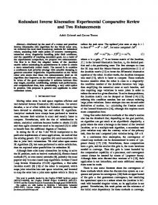
Figure 1: The link coordinates system of a five-axis articulated robot arm.
Table 1: Denavit-Hartenberg parameters for robot arm in Figure 1. Link 𝑖 1 2 3 4 5
𝑑𝑖 (mm) 𝑑1 = 275 0 0 0 𝑑5 = 195
𝑎𝑖 (mm) 0 𝑎2 = 275 𝑎3 = 255 0 0
𝛼𝑖 𝛼1 = −𝜋/2 0 0 𝛼4 = −𝜋/2 0
𝜃𝑖 𝜃1 𝜃2 𝜃3 𝜃4 𝜃5
0
2. Description of the Forward and Inverse Kinematics
0 0 1 0
0 cos 𝜃𝑖 − sin 𝜃𝑖 ] [ 0 ] [ sin 𝜃𝑖 cos 𝜃𝑖 ][ 0 𝑑𝑖 ] [ 0 1][ 0 0
0 0 1 0
0 0] ] ] 0] 1]
0 0] ] ] 0] 1]
3
0 0] ] ], 𝑑1 ] 1]
𝐴 2 = 𝑇 (𝑍, 0) 𝑇 (𝑍, 𝜃2 ) 𝑇 (𝑋, 𝑎2 ) 𝑇 (𝑋, 0) 0 𝑎2 cos 𝜃2 0 𝑎2 sin 𝜃2 ] ] ], 1 0 ] 0 1 ]
𝐴 3 = 𝑇 (𝑍, 0) 𝑇 (𝑍, 𝜃3 ) 𝑇 (𝑋, 𝑎3 ) 𝑇 (𝑋, 0) cos 𝜃3 − sin 𝜃3 [ sin 𝜃 cos 𝜃 [ 3 3 =[ [ 0 0 0 [ 0
0 𝑎3 cos 𝜃3 0 𝑎3 sin 𝜃3 ] ] ], 1 0 ] 0 1 ]
𝜋 𝐴 4 = 𝑇 (𝑍, 0) 𝑇 (𝑍, 𝜃4 ) 𝑇 (𝑋, 0) 𝑇 (𝑋, − ) 2 cos 𝜃4 [ sin 𝜃 [ 4 =[ [ 0 [ 0
4
0 1 0 0
0 − sin 𝜃1 0 cos 𝜃1 −1 0 0 0
cos 𝜃2 − sin 𝜃2 [ sin 𝜃 cos 𝜃 [ 2 2 =[ [ 0 0 0 [ 0 2
A typical five-axis articulated robot arm is studied in this paper. Figure 1 shows its link coordinate system by DenavitHartenberg convention. Table 1 illustrates the values of the kinematics parameters. The forward kinematics of the articulated robot arm is the transformation of joint space 𝑅5 (𝜃1 , 𝜃2 , 𝜃3 , 𝜃4 , 𝜃5 ) to Cartesian space 𝑅3 (𝑥, 𝑦, 𝑧). Conversely, the inverse kinematics of the articulated robot arm will transform the coordinates of robot manipulator from Cartesian space 𝑅3 (𝑥, 𝑦, 𝑧) to the joint space 𝑅5 (𝜃1 , 𝜃2 , 𝜃3 , 𝜃4 , 𝜃5 ). The computational procedure of forward and inverse kinematics is shown in Figure 1 and Table 1. A coordinate frame is assigned to each link based on Denavit-Hartenberg notation. The transformation matrix for each link from frame 𝑖 to 𝑖 − 1 is given by
1 [0 [ =[ [0 [0
1 0 0 𝑎𝑖 ] [ 0 ] [0 cos 𝛼𝑖 − sin 𝛼𝑖 ][ 0 ] [0 sin 𝛼𝑖 cos 𝛼𝑖 0 1 ] [0 0
𝜋 𝐴 1 = 𝑇 (𝑍, 𝑑1 ) 𝑇 (𝑍, 𝜃1 ) 𝑇 (𝑋, 0) 𝑇 (𝑋, − ) 2 cos 𝜃1 [ sin 𝜃 [ 1 =[ [ 0 [ 0
forward kinematics and inverse kinematics hardware. Some simulation results based on EDA simulator link will demonstrate the correctness and effectiveness of the forward and inverse kinematics.
𝐴 𝑖 = 𝑇 (𝑍, 𝑑) 𝑇 (𝑍, 𝜃) 𝑇 (𝑋, 𝑎) 𝑇 (𝑋, 𝛼)
0 0 1 0
where 𝑇(𝑍, 𝜃) and 𝑇(𝑋, 𝛼) present rotation and the 𝑇(𝑍, 𝑑) and 𝑇(𝑋, 𝛼) denote translation. Substituting the parameters in Table 1 into (1), the coordinate five matrixes respected with five axes of robot arm are shown as follows:
1
𝑖−1
0 1 0 0
cos 𝜃𝑖 − cos 𝛼𝑖 sin 𝜃𝑖 sin 𝛼𝑖 sin 𝜃𝑖 𝑎𝑖 cos 𝜃𝑖 [ sin 𝜃 cos 𝛼 cos 𝜃 − sin 𝛼 cos 𝜃 𝑎 sin 𝜃 ] [ 𝑖 𝑖 𝑖 𝑖 𝑖 𝑖 𝑖] =[ ], [ 0 sin 𝛼𝑖 cos 𝛼𝑖 𝑑𝑖 ] 0 0 1 ] [ 0 (1)
z5
y0
𝜃1
1 [0 [ ×[ [0 [0
a3
a2
0 − sin 𝜃4 0 cos 𝜃4 −1 0 0 0
0 0] ] ], 0] 1]
𝐴 5 = 𝑇 (𝑍, 𝑑5 ) 𝑇 (𝑍, 𝜃5 ) 𝑇 (𝑋, 0) 𝑇 (𝑋, 0) cos 𝜃5 − sin 𝜃5 [ sin 𝜃 cos 𝜃 [ 5 5 =[ [ 0 0 0 [ 0
0 0 1 0
0 0] ] ]. 𝑑5 ] 1] (2)
Mathematical Problems in Engineering
3
The forward kinematics of the end-effector with respect to the base frame is determined by multiplying five matrices from (2) as given above. An alternative representation of 0 𝐴5 can be written as 𝑅
0
0
1
2
3
𝑎𝑥 𝑎𝑦 𝑎𝑧 0
𝑝𝑥 𝑝𝑦 ] ] ]. 𝑝𝑧 ] 1]
of robot arm by always gripping from a top down position. Therefore, the matrix in (3) is set by the following form: 1 [ 0 𝑅 𝑇𝐻 = [ [0 [0
𝑇𝐻 = 𝐴 5 = 𝐴 1 ⋅ 𝐴 2 ⋅ 𝐴 3 ⋅ 𝐴 4 𝑛𝑥 [𝑛 [ 𝑦 ⋅ 4𝐴 5 Δ [ [𝑛𝑧 [0
𝑜𝑥 𝑜𝑦 𝑜𝑧 0
0 −1 0 0
0 0 −1 0
𝑥 𝑦] ]. 𝑧] 1]
(18)
Comparing the element (3,3) in (18) with (12), we obtained (3)
cos 𝜃234 = 1.
(19)
𝜃234 = 0.
(20)
Therefore, we can get
The (𝑛, 𝑜, 𝑎) are the orientation in the Cartesian coordinate system which is attached to the end-effector. Using the homogeneous transformation matrix to solve the kinematics problems, its transformation specifies the location (position and orientation) of the end-effector and the vector 𝑝 presents the position of end-effector of robot arm. By multiplying five matrices and substituting into (3) and then comparing all the components of both sides after that we can solve the forward kinematics of the five-axis articulated robot arm as follows:
Further, comparing the element (1,1) in (18) with (4), we obtained cos (𝜃1 − 𝜃5 ) = 1.
(21)
𝜃1 − 𝜃5 = 0 or 𝜃5 = 𝜃1 .
(22)
Therefore, we can get
Let us assume that 𝑏 = 𝑎2 cos 𝜃2 + 𝑎3 cos 𝜃23 ;
𝑛𝑥 = cos 𝜃1 cos 𝜃234 cos 𝜃5 + sin 𝜃1 sin 𝜃5 ,
(4)
𝑛𝑦 = sin 𝜃1 cos 𝜃234 cos 𝜃5 − cos 𝜃1 sin 𝜃5 ,
(5)
𝑛𝑧 = − sin 𝜃234 cos 𝜃5 ,
(6)
𝑜𝑥 = − cos 𝜃1 cos 𝜃234 sin 𝜃5 + sin 𝜃1 cos 𝜃5 ,
(7)
𝑜𝑦 = − sin 𝜃1 cos 𝜃234 sin 𝜃5 − cos 𝜃1 cos 𝜃5 ,
(8)
𝑜𝑧 = sin 𝜃234 sin 𝜃5 ,
(9)
𝑏 = ±√(𝑥2 + 𝑦2 ),
𝑎𝑥 = − cos 𝜃1 sin 𝜃234 ,
(10)
𝑎𝑦 = − sin 𝜃1 sin 𝜃234 ,
(11)
𝑦 𝜃1 = 𝜃5 = 𝑎 tan 2 ( ) . 𝑥
𝑎𝑧 = − cos 𝜃234 ,
(12)
𝑝𝑥 = cos 𝜃1 (𝑎2 cos 𝜃2 + 𝑎3 cos 𝜃23 − 𝑑5 sin 𝜃234 ) ,
(13)
𝑝𝑦 = sin 𝜃1 (𝑎2 cos 𝜃2 + 𝑎3 cos 𝜃23 − 𝑑5 sin 𝜃234 ) ,
(14)
𝑝𝑧 = 𝑑1 − 𝑎2 sin 𝜃2 − 𝑎3 sin 𝜃23 − 𝑑5 cos 𝜃234 ,
(15)
(23)
then substituting (19)∼(22) into (13)∼(15), we can get the sequence for computations inverse kinematics as follows: 𝑥 = cos 𝜃1 ⋅ 𝑏
(24)
𝑦 = sin 𝜃1 ⋅ 𝑏
(25)
𝑧 = 𝑑1 − 𝑎2 sin 𝜃2 − 𝑎3 sin 𝜃23 − 𝑑5 .
(26)
From (24) and (25), we can get
(27)
From (23) and (26), we can get 2
𝜃3 = arccos (
𝑏2 + (𝑑1 − 𝑑5 − 𝑧) − 𝑎22 − 𝑎32 ). 2𝑎2 𝑎3
(28)
Once 𝜃3 is obtained, substitute it to (23) and (26) to get 𝑏 = (𝑎2 + 𝑎3 cos 𝜃3 ) cos 𝜃2 + 𝑎3 sin 𝜃3 sin 𝜃2 , 𝑑1 − 𝑑5 − 𝑧 = (𝑎2 + 𝑎3 cos 𝜃3 ) sin 𝜃2 + 𝑎3 sin 𝜃3 cos 𝜃2 .
where
(29)
From (29), solve the linear equation in order to find the sin 𝜃2 and cos 𝜃2 as
𝜃23 = 𝜃2 + 𝜃3 ,
(16)
𝜃234 = 𝜃2 + 𝜃3 + 𝜃4 .
(17)
The position vector 𝑝 directs the location of the origin of the (𝑛, 𝑜, 𝑎) frame which is defined to let the end-effector
sin 𝜃2 = cos 𝜃2 =
(𝑎2 + 𝑎3 cos 𝜃3 ) (𝑑1 − 𝑑5 − 𝑧) − 𝑎3 𝑏 sin 𝜃3 𝑏2 + (𝑑1 − 𝑑5 − 𝑧)
2
,
(𝑎2 + 𝑎3 cos 𝜃3 ) 𝑏 + 𝑎3 sin 𝜃3 (𝑑1 − 𝑑5 − 𝑧) 𝑏2 + (𝑑1 − 𝑑5 − 𝑧)
2
(30) .
4
Mathematical Problems in Engineering
Therefore, 𝜃2 can be derived as follows: 𝜃2 = 𝑎 tan 2 [
(𝑎2 + 𝑎3 cos 𝜃3 ) (𝑑1 − 𝑑5 − 𝑧) − 𝑎3 𝑏 sin 𝜃3 ]. (𝑎2 + 𝑎3 cos 𝜃3 ) 𝑏 + 𝑎3 sin 𝜃3 (𝑑1 − 𝑑5 − 𝑧) (31)
Further, from (17) and (20), 𝜃4 is obtained as 𝜃4 = −𝜃2 − 𝜃3 .
(32)
Finally, the forward kinematics and inverse kinematics of the five-axis articulated robot arm, based on the assumption in (18) in which the end-effector of the robot arm is always toward the top down direction, can be summarized as follows. For computing the forward kinematics, consider the following steps. Step 1. Consider end 𝑥 = cos 𝜃1 (𝑎2 cos 𝜃2 + 𝑎3 cos 𝜃23 − 𝑑5 sin 𝜃234 ) .
(33)
Step 2. Consider end 𝑦 = sin 𝜃1 (𝑎2 cos 𝜃2 + 𝑎3 cos 𝜃23 − 𝑑5 sin 𝜃234 ) .
(34)
Step 3. Consider end 𝑧 = 𝑑1 − 𝑎2 sin 𝜃2 − 𝑎3 sin 𝜃23 − 𝑑5 cos 𝜃234 .
For computing the inverse kinematics, consider the following steps. Step 1. Consider (36)
Step 2. Consider 𝑏 = ±√end 𝑥2 + end 𝑦2 .
(37)
Step 3. Consider 2
𝜃3 = 𝑎 cos (
𝑏2 + (𝑑1 − 𝑑5 − end 𝑧) − 𝑎22 − 𝑎32 ). 2𝑎2 𝑎3
(38)
Step 4. Consider 𝑆2 = (𝑎2 + 𝑎3 cos 𝜃3 ) (𝑑1 − 𝑑5 − end 𝑧) − 𝑎3 𝑏 sin 𝜃3 .
(39)
Step 5. Consider 𝐶2 = (𝑎2 + 𝑎3 cos 𝜃3 ) 𝑏 + 𝑎3 sin 𝜃3 (𝑑1 − 𝑑5 − end 𝑧) .
Before performing the computation of the forward and inverse kinematics for five-axis articulated robot arm, some key trigonometric functions need to be built up as a component for being applied, and those are sine function, cosine function, arctangent function, and arccosine function. To increase the computing accuracy, LUT (look-up table) technique and Taylor series expanse technique are used to the computational algorithm design of the arctangent function and arccosine function. However, the computation algorithm used in these two functions is very similar; therefore, the detailed design methods, only sine/cosine function, and arctangent function are described as follows. 3.1. Computation Algorithm and Hardware Realization of Sine Function and Cosine Function. To compute sin(𝜃) and cos(𝜃) functions, the 𝜃 = 𝜃𝐼 + 𝜃𝐹 is firstly defined, in which 𝜃𝐼 and 𝜃𝐹 represented the integer part and fraction part of the 𝜃, respectively. Then the formulation of these two functions is expanded as follows: sin (𝜃𝐼 + 𝜃𝐹 ) = sin (𝜃𝐼 ) cos (𝜃𝐹 ) + cos (𝜃𝐼 ) sin (𝜃𝐹 )
(35)
In the previous steps, end 𝑥, end 𝑦, and end 𝑧 are the position of end point which are the same as 𝑥, 𝑦, and 𝑧 in (18).
𝜃1 = 𝜃5 = 𝑎 tan 2 (end 𝑦, end 𝑥) .
3. Computations of Trigonometric Function and Its Hardware Implementation
(40)
Step 6. Consider 𝜃2 = 𝑎 tan 2 (𝑆2 , 𝐶2 ) .
(41)
𝜃4 = −𝜃2 − 𝜃3 .
(42)
Step 7. Consider The parameters of robot arm 𝑎2 , 𝑎3 , 𝑑1 , 𝑑5 are shown in Table 1.
cos (𝜃𝐼 + 𝜃𝐹 ) = cos (𝜃𝐼 ) cos (𝜃𝐹 ) − sin (𝜃𝐼 ) sin (𝜃𝐹 ) .
(43)
In the hardware design, 𝜃 is adopted as 16-bit Q7 format. Therefore, if 𝜃 is 0000001001000000, it represents 4.5 degree. In addition, four LUTs (look-up tables) are built up to store the values of sin (𝜃𝐼 ), cos (𝜃𝐼 ), sin (𝜃𝐹 ), and cos (𝜃𝐹 ) functions. The LUT for sin (𝜃𝐼 ) and cos (𝜃𝐼 ) functions stores 360 pieces of data with 24-bit Q23 format and that for sin (𝜃𝐹 ) and cos (𝜃𝐹 ) functions stores 128 pieces of data with the same 24bit Q23 format. Therefore, according to (43), the results of sine and cosine with 16-bit Q15 format can be computed after looking up four tables. In the realization, finite state machine (FSM) is adopted and the example to compute the cosine function is shown in Figure 2. It presents four LUTs, two multipliers, and one adder in hardware which manipulates 6 steps to complete the overall computation. Due to the fact that the operation of each step is 20 ns (50 MHz) in FPGA, a total of 6 steps only need 120 ns operation time. In addition, the FPGA (Altera Cyclone IV) resource usage for the realization of the sine or cosine function needs 232 logic elements (LEs) and 30,720 RAM bits. 3.2. Computation Algorithm and Hardware Realization of Arctangent Function. The equation of arctangent function is shown as follows: 𝑦 (44) 𝜃 = 𝑎 tan 2 ( ) , 𝑥 where the inputs are 𝑥 and 𝑦 and the output is 𝜃. Herein, there are two steps to evaluate the arctangent function. (1) First Step. 𝜃1 = 𝑓(𝑥) = tan−1 (𝑥) is computed by using Taylor series expansion and the input values are defined within 1 ≤ 𝑥 ≤ 0 (or the output value: 45∘ ≤ 𝜃1 ≤ 0∘ ).
Mathematical Problems in Engineering
5 y
𝜃(15· ·7)
mult r1(46· ·23)
LUT (cos)
×
LUT (dcos) 𝜃(6· ·0)
−y 𝜃 = 180∘ − tan−1 ( ) x
+
LUT (sin)
−
−y 𝜃 = −180∘ + tan−1 ( ) −x
mult r2(46· ·23) S1
III
x 𝜃 = 90∘ − tan−1 ( ) y
y 𝜃 = tan−1 ( ) x
II I
IV
x
×
LUT (dsin) S0
Cos 16 = addr1(23· ·8)
−x 𝜃 = 90∘ + tan−1 ( ) y
S2
S3
S4
V
VIII VI
VII
−y 𝜃 = −tan−1 ( ) x
S5
Figure 2: FSM for computing the cosine function.
−x 𝜃 = −90∘ − tan−1 ( ) 𝜃 = −90∘ + tan−1 ( x ) −y −y
The third-order polynomial is considered and the expression within the vicinity of 𝑥0 is shown as follows:
Figure 3: Compute 𝜃 = 𝑎 tan 2(𝑦/𝑥) of each region in 𝑋-𝑌 coordinates.
2
3
𝑓 (𝑥) ≅ 𝑎0 + 𝑎1 (𝑥 − 𝑥0 ) + 𝑎2 (𝑥 − 𝑥0 ) + 𝑎3 (𝑥 − 𝑥0 ) , (45) with 𝑎0 = 𝑓 (𝑥0 ) = tan−1 (𝑥0 ) , 𝑎1 = 𝑓 (𝑥0 ) =
1 , 1 + 𝑥02
𝑎2 = 𝑓 (𝑥0 ) =
−2𝑥0
𝑎3 = 𝑓(3) (𝑥0 ) =
(1 +
(46)
,
2 𝑥02 )
−2 + 6𝑥02
3
(1 + 𝑥02 )
.
Actually, in realization, only third-order expansion in (44) is not enough to obtain an accuracy approximation due to the reason that the large error will occur when the input 𝑥 is far from 𝑥0 . To solve this problem, combining the LUT technique and Taylor series expanse technique is considered. To set up the LUT, several specific values for 𝑥0 within the range 1 ≤ 𝑥 ≤ 0 are firstly chosen; then the parameters from 𝑎0 to 𝑎3 in (46) are computed. Those data included 𝑥0 and 𝑎0 to 𝑎3 will be stored to LUT. Following that, when it needs to compute tan−1 (𝑥) in (45), the 𝑥0 which is the most approximate to input 𝑥 and its related 𝑎0 to 𝑎3 will be selected from LUT and then perform the computing task. (2) Second Step. After completing the computation of tan−1 (𝑥), we can evaluate 𝜃 = 𝑎 tan 2(𝑦/𝑥) further and let the output suitable to the range be within −180∘ ≤ 𝜃 ≤ 180∘ . The formulation for each region in 𝑋-𝑌 coordinate is shown in Figure 3. In hardware implementation, the inputs and output of the arctangent function are designed with 32-bit Q15 and 16bit Q15 format, respectively. It consists of one main circuit with FSM architecture and two components for computing the divider and tan−1 (𝑥) functions. However, the design and implementation of the tan−1 (𝑥) function is a major task. The input and output values of component tan−1 (𝑥) all belong
𝜃 = tan−1 (x) ≅ a0 + a1 (x − x0 ) + a2 (x − x0 )2 + a3 (x − x0 )3 xx addr = xx(14· · 11) dxx mult r1(30· · 15) − LUT + (x0 ) saa1 x0 × + saa2 a 1 LUT + a0 (a1 ) sita dxx a2 + × LUT a0 2 dxx (a0) × dxx3 LUT a2 × × (a2 ) dxx dxx mult r1(30· · 15) LUT a3 a3 (a3 ) S0 S1 S2 S3 S4 S5 S6
Figure 4: FSM to compute tan−1 (𝑥) function.
to 16-bit Q15 format. The FSM is employed to model the computation of tan−1 (𝑥) and is shown in Figure 4 which uses two multipliers and one adder in the design. The multiplier and adder apply Altera LPM (library parameterized modules) standard. In Figure 4, it manipulates 7-step machine to carry out the overall computations of tan−1 (𝑥). The steps 𝑠0 ∼ 𝑠1 execute to look up 5 tables and 𝑠2 ∼ 𝑠6 perform the computation of polynomial in (45). Further, according to the computation logic shown in Figure 3, it uses 16 steps to complete the 𝑎 tan 2(𝑦/𝑥) function. Due to the fact that the operation of each step is 20 ns (50 MHz) in FPGA, a total of 16 steps only need 320 ns operation time. In addition, the FPGA (Altera Cyclone IV) resource usage for the realization of the arctangent function needs 4,143 LEs and 1,280 RAM bits.
4. Design and Hardware Implementation of Forward/Inverse Kinematics and Its Simulation Results The block diagram of kinematics for five-axis articulated robot arm is shown in Figure 5. The inputs are the endpoint position by end 𝑥, end 𝑦, and end 𝑧 which is relative
6
Mathematical Problems in Engineering
𝜃1 (15 : 0) end x(31 : 0)
𝜃2 (15 : 0)
end y(31 : 0)
𝜃3 (15 : 0) end x(31 : 0)
𝜃4 (15 : 0)
𝜃1 (15 : 0)
end z(31 : 0)
𝜃2 (15 : 0)
end y(31 : 0)
𝜃5 (15 : 0)
𝜃3 (15 : 0)
end z(31 : 0) a2 (31 : 0) a3 (31 : 0)
a2 (31 : 0)
𝜃4 (15 : 0)
a3 (31 : 0)
𝜃5 (15 : 0)
d1 (31 : 0)
d1 (31 : 0)
d5 (31 : 0)
d5 (31 : 0) (a)
(b)
Figure 5: Block diagram for (a) forward kinematics and (b) inverse kinematics.
𝜃1
𝜃234
COM cos𝜃1 for cos
𝜃2 COM cos𝜃2 𝜃3 𝜃23 × for cos + 𝜃234 M1 𝜃2 A1 + a2 A1 𝜃4 𝜃1 COM sin𝜃1 a2 for sin 𝜃2 M2 COM × for sin sin𝜃 2 𝜃23
COM for cos
COM for cos
var1
cos𝜃234 var9 + × M1 A1 d5 var8
var89
d5 var4 end x var34 M2 × + COM × M1 − for sin sin𝜃 A2 234 cos𝜃1 var6 𝜃234
×
var1
cos𝜃23 var2 × M1 a3
+
var3
sin𝜃1 var89 var16 var6 − end z + − M1 + A2 d1
a3
𝜃23 COM M2 var8 × for sin sin𝜃23 S0
S1
S2∼
S7
S8∼
S15∼
S21
S22∼
end y
S28
S29
S30
S31
S32
S33
Figure 6: FSM for computing the forward kinematics.
to (𝑥, 𝑦, 𝑧), as well as the mechanical parameters by 𝑎2 , 𝑎3 , 𝑑1 , and 𝑑5 . The outputs are mechanical angles 𝜃1 ∼ 𝜃5 . In Figure 5, the parameters of mechanical length and the endpoint position are designed with 32-bit Q15 data format and the parameters of mechanical angle are designed with 16-bit Q7 data format. According to the formulations of forward and inverse kinematics which are described in Section 2, the finite state machine (FSM) method is applied to design the hardware for reducing the usage of hardware resource. Herein, the FSM designs to compute the forward kinematics and inverse kinematics are, respectively, shown in Figures 6 and 7. The FSM will generate sequential signals and will step-by-step compute the forward kinematics and inverse kinematics. The implementation of inverse kinematics is developed by VHDL.
In Figure 6, there are 34 steps to present the computations of forward kinematics, and the circuit includes two multipliers, two adders, one component for sine function, and one component for cosine function. In Figure 7, there are 47 steps to perform the inverse kinematics, and the circuit needs three multipliers, two dividers, two adders, one square root function, one component for arctangent function, one component for arccosine function, one component for sine function, and one component for cosine function. The notation “COM” in Figures 6∼7 is represented with “component.” For example, the “COM for cos” is the component of cosine function. The designs of the component regarded as trigonometric function are described in previous section. Due to the fact that the operation of each step is 20 ns (50 MHz) in FPGA,
Mathematical Problems in Engineering
7
d1 − d5 2 2 var12 a2 + a3 2a2 a3 end z − var1 + × M1 A1 end y ÷ + + end y2 × A1 A2 D2 var22 M2 + end x2 A1 √ end x × S1 M1
end y/end x
÷ D1
S0
S1
S2
a2
a3 var3 var6 × M3 COM for acos
+ A1
var5 𝜃3
var4
var2 𝜃1 , 𝜃5
COM for atan2
S4
S3
var2 var5 × C2 M1 var1 + var1 A1 var7 var5 × × M2 M1 S2 a3 var2 ÷ − var4 var7 D1 × × + M3 M2 A1 S23 S24 S25 S26 S27
sin𝜃3
COM for sin
S5∼
S2 /C2
S6
S7
S8∼
S16
𝜃3 𝜃2 −− +
COM for atan2
S28
S29
S20
S17∼
S40
∼
S44
S45
S23
𝜃4
S46
Figure 7: FSM for computing the inverse kinematics.
the executing time for the computation of forward and inverse kinematics is 680 ns and 940 ns, respectively. In addition, the FPGA (Altera Cyclone IV) resource usage for the realization of the forward kinematics IP and the inverse kinematics IP is 1,575 LEs and 30,720 RAM bits and 9,400 LEs and 84,224 RAM bits, respectively. The cosimulation architecture by ModelSim/SimuLink for the proposed forward kinematics is shown in Figure 8 and that for the inverse kinematics is shown in Figure 9, whose works in ModelSim execute the function of the computing the forward and inverse kinematics. The input values to ModelSim are provided from Simulink and, through the computation working in ModelSim, output responses are displayed to Simulink. To confirm the correctness, an embedded Matlab function for computing the forward and inverse kinematics is considered. Under the cosimulation of ModelSim and Simulink architecture, the simulation results are presented as follows. Mechanical parameters of the five-axis articulated robot arm are chosen by 𝑎2 = 275,
𝑎3 = 255,
In the second case, the inputs end 𝑥, end 𝑦, and end 𝑧 are chosen as end 𝑥 = 60,
end 𝑦 = 180,
end 𝑧 = 450.
Simulation results of forward kinematics with the following two cases are listed in Table 3. The inputs of forward kinematics are five joint angles presented by 𝜃1 , 𝜃2 , 𝜃3 , 𝜃4 , 𝜃5 (degree) and the outputs are end-effectors presented by end 𝑥, end 𝑦, and end 𝑧 (mm). In the first case, the inputs 𝜃1 , 𝜃2 , 𝜃3 , 𝜃4 , and 𝜃5 are chosen as 𝜃1 = 44.9043477, 𝜃3 = 49.1952721,
𝜃2 = 4.8948685, 𝜃4 = −54.0901472,
In the second case, the inputs 𝜃1 , 𝜃2 , 𝜃3 , 𝜃4 , and 𝜃5 are chosen as 𝜃1 = 71.5650511,
𝜃2 = −99.4939347,
Simulation results of inverse kinematics with the following two cases are listed in Table 2. The inputs of inverse kinematics are the end-effectors of robot arm presented by end 𝑥, end 𝑦, and end 𝑧 (mm) and the outputs are five joint angles presented by 𝜃1 , 𝜃2 , 𝜃3 , 𝜃4 , 𝜃5 (degree). In the first case, the inputs end 𝑥, end 𝑦, and end 𝑧 are chosen as end 𝑥 = 300, end 𝑦 = 299, (48) end 𝑧 = −150.
𝜃3 = 76.703125,
𝜃4 = 22.7812500,
𝑑5 = 195 (mm) .
(50)
𝜃5 = 44.9043477.
(47)
𝑑1 = 275,
(49)
(51)
𝜃5 = 71.5650511. From these two cases, the absolute difference of end-effectors end 𝑥, end 𝑦, and end 𝑧 which are calculated from ModelSim and from Matlab is less than 0.05 mm, and 𝜃1 to 𝜃5 are less than 0.01∘ . It shows that the proposed forward and inverse kinematics for the five-axis articulated robot arm are correct and effective.
8
Mathematical Problems in Engineering
71.5650511 𝜃1
Convert
𝜃1
−99.4939347 𝜃2
Convert
𝜃2
76.7060765 𝜃3
Convert
𝜃3
22.7878581 𝜃4
Convert
𝜃4
71.5650511
Convert
𝜃5
𝜃5 275 a2
Convert
a2
255 a3
Convert
a3
275 d1
Convert
d1
195 d5
Convert
d5
ModelSim
1965798
Q15 of x end x
K− Gain3
59.991394042969 end x − +
0.0086063533472114 Erorr of X
5897963 Q15 of y end y
K− Gain1
179.99154663086
end y − +
0.0084537509296467 Erorr of Y
14746840 Q15 of z end z
K− Gain2
450.03784179688 end z
− +
−0.037841604891696 Erorr of Z
Forward kinematics 𝜃1 𝜃2
end x
60.000000396316 end x
end y
180.00000038179
𝜃3 𝜃4 𝜃5 a2
fcn
end y
a3 d1
450.00000019198
end z
end z
d5 Embedded Matlab function
Figure 8: Cosimulation architecture of forward kinematics using ModelSim and SimuLink. Table 2: Two cases’ simulation results of inverse kinematics from ModelSim and Matlab. Input Output 𝜃1 𝜃2 𝜃3 𝜃4 𝜃5
The 1st case (end 𝑥, end 𝑦, end 𝑧)(1) ModelSim Matlab Error 44.8984375 44.9043477 0.0059702 4.8906250 4.8948685 0.0042435 49.1953125 49.1952721 −0.0000400 −54.0859375 −54.0901472 0.0042032 44.8984375 44.9043477 0.0059102
The 2nd case (end 𝑥, end 𝑦, end 𝑧)(2) ModelSim Matlab Error 71.5703125 71.5650511 −0.0052613 −99.4843750 −99.4939347 0.0095597 76.7060765 76.7031250 0.0029515 22.7878581 22.7812500 0.0066081 71.5703125 71.5650511 0.0052613
(1) denotes the case 1 shown in (48). (2) denotes the case 2 shown in (49).
Table 3: Two cases’ simulation results of forward kinematics from ModelSim and Matlab. Input Output end 𝑥 end 𝑦 end 𝑧
The 1st case (𝜃1 , 𝜃2 , 𝜃3 , 𝜃4 , 𝜃5 )(1) ModelSim Matlab Error 300.0321650 300.0000160 −0.0321490 299.0496215 299.0000160 −0.0496054 −149.9700920 −149.9999999 −0.0299906
(1) denotes the case 1 shown in (50). (2) denotes the case 2 shown in (51).
The 2nd case (𝜃1 , 𝜃2 , 𝜃3 , 𝜃4 , 𝜃5 )(2) ModelSim Matlab Error 59.9913940 60.0000000 0.0086063 179.9915466 180.0000000 0.0084537 450.0378417 450.0000000 −0.0378416
Mathematical Problems in Engineering
9
60 x
Convert
end x
180 y
Convert
end y
450 z
Convert
275 a2
Convert
a2
255 a3
Convert
a3
275 d1
Convert
d1
195
Convert
d5
ModelSim
𝜃1
𝜃2 end z
𝜃3
𝜃4
𝜃5
K− Gain1
K− Gain2
K− Gain3
− +
− +
K− Gain4
K− Gain5
d5
71.5703125 𝜃1
− +
− +
− +
−0.00526132292201
Erorr of 𝜃1
−99.484375 𝜃2
−0.0095597449695077 Erorr of 𝜃2
76.703125 𝜃3
0.0029515830817672 Erorr of 𝜃3
22.78125 𝜃4
0.0066081618877369 Erorr of 𝜃4
71.5703125 𝜃5
−0.00526132292201 Erorr of 𝜃5
Inverse kinematics end x
71.565051177078
𝜃1
𝜃1 m
end y
a2
−99.49393474497
𝜃2
end z
𝜃2 m fcn
76.706076583082
𝜃3
𝜃3 m a3
22.787858161888
𝜃4
𝜃4 m
d1
71.565051177078
𝜃5
d5
𝜃5 m Embedded Matlab function
Figure 9: Cosimulation architecture of inverse kinematics using ModelSim and SimuLink.
5. Conclusions
Conflict of Interests
The forward kinematics and inverse kinematics of five-axis articulated robot arm, in which the end-effector of the robot arm is always toward the top down direction, have been successfully demonstrated in this paper. Through the cosimulation of ModelSim and Simulink, the accuracy under two examples of forward and inverse kinematics with the results of error of the end-effectors end 𝑥, end 𝑦, and end 𝑧 is less than 0.05 mm and the error for 𝜃1 ∼ 𝜃5 is less than 0.01∘ . Further, the executing times for the computations of forward and inverse kinematics in FPGA are only 680 ns and 940 ns, respectively. The high speed computational power and reasonable accuracy apparently increase the motion performance of the five-axis articulated robot arm.
The authors declare that there is no conflict of interests regarding the publication of this paper.
Acknowledgment This work was supported by National Science Council of the R.O.C. under Grant no. NSC 100-2632-E-218 -001-MY3.
References [1] J. J. Craig, Introduction to Robotics, Mechanics & Control, Addison-Wesley, New York, NY, USA, 1986.
10 [2] W. Shen, J. Gu, and E. E. Milios, “Self-configuration fuzzy system for inverse kinematics of robot manipulators,” in Proceedings of the Annual Meeting of the North American Fuzzy Information Processing Society (NAFIPS ’06), pp. 41–45, June 2006. [3] P. Falco and C. Natale, “On the stability of closed-loop inverse kinematics algorithms for redundant robots,” IEEE Transactions on Robotics, vol. 27, no. 4, pp. 780–784, 2011. [4] S.-W. Park and J.-H. Oh, “Hardware realization of inverse kinematics for robot manipulators,” IEEE Transactions on Industrial Electronics, vol. 41, no. 1, pp. 45–50, 1994. [5] G.-S. Huang, C.-K. Tung, H.-C. Lin, and S.-H. Hsiao, “Inverse kinematics analysis trajectory planning for a robot arm,” in Proceedings of the 8th Asian Control Conference (ASCC ’11), pp. 965–970, twn, May 2011. [6] E. Monmasson, L. Idkhajine, M. N. Cirstea, I. Bahri, A. Tisan, and M. W. Naouar, “FPGAs in industrial control applications,” IEEE Transactions on Industrial Informatics, vol. 7, no. 2, pp. 224–243, 2011. [7] J. U. Cho, Q. N. Le, and J. W. Jeon, “An FPGA-based multipleaxis motion control chip,” IEEE Transactions on Industrial Electronics, vol. 56, no. 3, pp. 856–870, 2009. [8] Y.-S. Kung, K.-H. Tseng, C.-S. Chen, H.-Z. Sze, and A.-P. Wang, “FPGA-implementation of inverse kinematics and servo controller for robot manipulator,” in Proceedings of the IEEE International Conference on Robotics and Biomimetics (ROBIO ’06), pp. 1163–1168, December 2006. [9] S. S´anchez-Solano, A. J. Cabrera, I. Baturone, F. J. MorenoVelo, and M. Brox, “FPGA implementation of embedded fuzzy controllers for robotic applications,” IEEE Transactions on Industrial Electronics, vol. 54, no. 4, pp. 1937–1945, 2007. [10] C. C. Wong and C. C. Liu, “FPGA realisation of inverse kinematics for biped robot based on CORDIC,” Electronics Letters, vol. 49, no. 5, pp. 332–334, 2013. [11] The Mathworks, Matlab/Simulink Users Guide, Application Program Interface Guide, 2004. [12] Modeltech, ModelSim Reference Manual, 2004. [13] Y.-S. Kung, N. V. Quynh, C.-C. Huang, and L.-C. Huang, “Simulink/ModelSim co-simulation of sensorless PMSM speed controller,” in Proceedings of the IEEE Symposium on Industrial Electronics and Applications (ISIEA ’11), pp. 24–29, September 2011.
Mathematical Problems in Engineering
Advances in
Operations Research Hindawi Publishing Corporation http://www.hindawi.com
Volume 2014
Advances in
Decision Sciences Hindawi Publishing Corporation http://www.hindawi.com
Volume 2014
Journal of
Applied Mathematics
Algebra
Hindawi Publishing Corporation http://www.hindawi.com
Hindawi Publishing Corporation http://www.hindawi.com
Volume 2014
Journal of
Probability and Statistics Volume 2014
The Scientific World Journal Hindawi Publishing Corporation http://www.hindawi.com
Hindawi Publishing Corporation http://www.hindawi.com
Volume 2014
International Journal of
Differential Equations Hindawi Publishing Corporation http://www.hindawi.com
Volume 2014
Volume 2014
Submit your manuscripts at http://www.hindawi.com International Journal of
Advances in
Combinatorics Hindawi Publishing Corporation http://www.hindawi.com
Mathematical Physics Hindawi Publishing Corporation http://www.hindawi.com
Volume 2014
Journal of
Complex Analysis Hindawi Publishing Corporation http://www.hindawi.com
Volume 2014
International Journal of Mathematics and Mathematical Sciences
Mathematical Problems in Engineering
Journal of
Mathematics Hindawi Publishing Corporation http://www.hindawi.com
Volume 2014
Hindawi Publishing Corporation http://www.hindawi.com
Volume 2014
Volume 2014
Hindawi Publishing Corporation http://www.hindawi.com
Volume 2014
Discrete Mathematics
Journal of
Volume 2014
Hindawi Publishing Corporation http://www.hindawi.com
Discrete Dynamics in Nature and Society
Journal of
Function Spaces Hindawi Publishing Corporation http://www.hindawi.com
Abstract and Applied Analysis
Volume 2014
Hindawi Publishing Corporation http://www.hindawi.com
Volume 2014
Hindawi Publishing Corporation http://www.hindawi.com
Volume 2014
International Journal of
Journal of
Stochastic Analysis
Optimization
Hindawi Publishing Corporation http://www.hindawi.com
Hindawi Publishing Corporation http://www.hindawi.com
Volume 2014
Volume 2014