Computing Randomized Security Strategies in Networked Domains Joshua Letchford∗
Yevgeniy Vorobeychik
Department of Computer Science Duke University Durham, NC, 27708
[email protected]
Sandia National Laboratories Livermore, CA 94551-0969
[email protected]
Abstract Traditionally, security decisions have been made without explicitly accounting for adaptive, intelligent attackers. Recent game theoretic security models have explicitly included attacker response in computing randomized security policies. Techniques to date, however, generally fail to explicitly account for interdependence between the targets to be secured, which is of vital importance in a variety of domains, including cyber, supply chain, and critical infrastructure security. We introduce a novel framework for computing optimal randomized security policies in networked domains which extends previous approaches in two ways. First, we extend previous linear programming techniques for Stackelberg security games to incorporate benefits and costs of arbitrary security configurations on individual assets. Second, we offer a principled model of failure cascades that allows us to capture both the direct and indirect value of assets. Finally, we use our framework to analyze four models, two based on random graph generation models, a simple model of interdependence between critical infrastructure and key resource sectors, and a model of the Fedwire interbank payment network.
1
Introduction
Game theoretic approaches to security have received much attention in recent years. Most have attempted to distill various aspects of the problem into a model that could then be solved in closed form (see, for example, a recent survey of game theoretic techniques applied to network security (Roy et al. 2010)). Numerous others, however, offer techniques based on mathematical programming to solve actual instances of security problems. Approaches to network interdiction (Cormican, Morton, and Wood 1998), for example, offer (usually) an integer programming formulation solving for an location of sensors that optimally interdict traffic (such as drug traffic) through a network. The point of departure of our work is a different line of work that develops linear and integer programming methods for optimal randomized allocation of security resources among possible attack targets. In this work, the assumption is made that the defender is a Stackelberg leader, that is, he is able to commit ∗ This paper represents work done while at Sandia National Laboratories c 2011, Association for the Advancement of Artificial Copyright Intelligence (www.aaai.org). All rights reserved.
to a randomized policy, which is subsequently observed by the attacker who optimally responds to it. Initial work on the subject offered an approach relying on multiple linear programs to compute such an optimal commitment strategy in general two-player games (Conitzer and Sandholm 2006). Follow-up work focused on integer programming methods for Bayesian security settings (Paruchuri 2008), and much has attempted to exploit the special structure of security scenarios to build faster algorithms (Kiekintveld et al. 2009), with some of these finding use in actual security applications such as ARMOR for the allocation of canine patrols in LAX and IRIS for the scheduling of federal air marshalls (Jain et al. 2010). In this paper we introduce a novel framework for computing optimal randomized security policies in networked domains. First, in Section 2 we give some background on how security scenarios have previously been modeled as Stackelberg games. We then propose an extension to this line of work, where rather than having a hard constraint on the number of defense resources we have a soft constraint in the form of costs. In Section 3 we extend previous linear programming techniques for Stackelberg security games to incorporate benefits and costs of arbitrary security configurations on individual assets. In Section 4 we offer a principled model of failure cascades that allows us to capture both the direct and indirect value of assets. In Section 5 we illustrate our model with a simple supply chain example. Finally, in Section 6 we use our model to study security decisions in four types of networks, two based on models of random graph generation, a simple model of interdependence between critical infrastructure and key resource sectors and a model of the Fedwire interbank payment network.
2
Stackelberg Security Games
A Stackelberg security game (Kiekintveld et al. 2009) consists of two players, the leader (defender) and the follower (attacker), and a set of possible targets. The leader can decide upon a randomized policy of defending the targets, possibly with limited defense resources; we say that the leader thereby commits to a mixed strategy. The follower (attacker) is assumed to observe the randomized policy of the leader, but not the realized defense actions. Upon observing the leader’s strategy, the follower chooses a target so as to maximize its expected utility.
In past work, Stackelberg security game formulations focused on defense policies that were costless, but resource bounded. Specifically, it had been assumed that the defender has K fixed resources available with which to cover (subsets of) targets. Additionally, security decisions amounted to covering a set of targets, or not. While in numerous settings to which such work has been applied (e.g., airport security, federal air marshall scheduling) this formulation is very reasonable, in other settings one may choose among many security configurations for each valued asset, and, additionally, security resources are only available at some cost. For example, in cybersecurity, protecting computing nodes could involve setting anti-virus and/or firewall configuration settings, with stronger settings carrying a benefit of better protection, but at a cost of added inconvenience, lost productivity, as well as possible licensing costs. Indeed, costs on resources may usefully take place of resource constraints, since such constraints are often not hard, but rather channel an implicit cost of adding further resources. To formalize, suppose that the defender can choose from a finite set O of security configurations for each target t ∈ T , with |T | = n. A configuration o ∈ O for target t ∈ T incurs a cost co,t to the defender. If the attacker happens to attack t while configuration o is in place, the expected value to the defender is denoted by Uo,t , while the attacker’s value is Vo,t . A key assumption in Stackelberg security games is that the targets are completely independent: that is, a joint defender and attacker decision concerning one target has no impact on the values of others, and total defender and attacker utilities are additive over all targets. We revisit this assumption below when we turn to networked (and general interdependent) settings. We denote by qo,t the probability that the defender chooses o at target t, while at denotes the probability that the attacker attacks target t.
3
Computing Optimal Randomized Security Configurations
Kiekintveld et al. (2009) previously introduced the ERASER algorithm, which is a Mixed Integer Programming (MIP) formulation for computing optimal randomized security policies in Stackelberg security games. We first show how to extend this MIP formulation to arbitrary security configurations, as well as to incorporate costs of such configurations. We then proceed to offer an alternative formulation involving multiple linear programs (in the same vein as the initial multiple-LP formulation for general Stackelberg games (Conitzer and Sandholm 2006)) and, finally, formulate this problem as a single linear program.
3.1
Mixed Integer Programming Formulation
The MIP formulation is shown in Equations 1- 7. Equations 2 and 3 force the attack vector to attack a single target with probability 1. This captures the well-known observation that a deterministic choice of the best of n targets to attack is optimal for the attacker (Kiekintveld et al. 2009). Equations 4 and 5 force the configuration decision for each target to be a valid probability distribution over O. In Equations 6 and 7, Z is some constant which is larger than the highest util-
ity achievable in the game. Consequently, Equation 6 will only bind when at = 1. This, combined with the fact that u is maximizedPin the objective, implies that in an optimal solution, u = o Uo,t · qo,t for the target that is attacked. Consequently, u corresponds to the optimal expected utility of the defender. The right-hand-side of Equation 7 will similarly only bind when at = 1. Since v is forced by the left-hand-side of Equation 7 to be at least the expected attacker utility from attacking any target, and must be exactly equal to the expected utility of the attacked target, it must therefore be the attacker’s optimal expected utility given the defender’s mixed strategy commitment q. XX max u− co,t · qo,t (1) t
o
s.t. ∀t X
at ∈ {0, 1}
(2)
at = 1
(3)
t
∀o,t X
∀t
qo,t ∈ [0, 1]
(4)
qo,t = 1
(5)
o
∀t
u−
X
Uo,t · qo,t ≤ (1 − at ) · Z
(6)
Vo,t · qo,t ≤ (1 − at ) · Z
(7)
o
∀t
0≤v−
X o
3.2
Multiple-LP Formulation
In reformulating the MIP above as a collection of LPs, we note that the lone integer vector a in the MIP formulation does not have combinatorial structure. Rather, it chooses a single target from n possibilities. Considering each of these possibilities for attack separately then yields n linear programs, and the defender can simply choose the solution with the highest expected value (u) as the optimal mixed strategy commitment. The resulting formulation as n LPs is shown in Equations 8-11. ∀tˆ max
X
ˆ
t Uo,tˆqo, − tˆ
o
XX t
ˆ
t co,t qo,t
(8)
o
s.t. ˆ
t qo,t ∈ [0, 1]
∀o,t X
∀t
tˆ qo,t
(9)
=1
(10)
o
∀t
X o
ˆ
t Vo,t qo,t ≤
X
ˆ
t Vo,tˆqo, tˆ
(11)
o
Notice that since the potential target is identified in each of n linear programs, we are able to compress the set of constraints, removing the now-redundant variables u and v. Each program now has a clean interpretation, just as in the original multiple-LP formulation due to Conitzer and Sandholm: for each target, we force the attacker to prefer that target over all others. The intuition behind this is that in an
optimal solution, the attacker must (weakly) prefer to attack some target, and consequently, one of these LPs must correspond to an optimal defense policy.
3.3
t0
Single Linear Program Formulation
Starting with the multiple-LP formulation above, it is now not difficult to construct just a single LP that aggregates all of these. We cannot do so immediately, however, because some of the n LPs may actually be infeasible: some targets may not be optimal for the attacker for any defense policy. Consequently, we must prune out all such targets in order to ensure that the combined LP is feasible. Formally, it suffices to check, for each target tˆ that max Vo,tˆ ≥ max min Vo,t , o
t
(12)
o
that is, that tˆ is not strictly dominated for the attacker. Let Tˆ ⊂ T be the set of targets for which Equation 12 holds. The aggregate single-LP formulation is then shown in Equations 13-16. ! X X XX ˆ ˆ t t max Uo,tˆqo, − co,t qo,t (13) tˆ tˆ∈Tˆ
o
t
o
s.t. ˆ
∀tˆ,o,t X
∀tˆ,t
t qo,t ∈ [0, 1]
(14)
tˆ qo,t
(15)
=1
o
∀tˆ,t
X
ˆ
t ≤ Vo,t qo,t
o
X
ˆ
t Vo,tˆqo, tˆ
(16)
o
Notice that we can easily incorporate additional linear constraints in any of these formulations. For example, it is often useful to add a budget constraint: X tˆ ≤ B. ∀tˆ,t co,t qo,t o
Below we utilize this single-LP formulation, without the budget constraint.
4
additive in target-specific worths. The expected utility Uo,t is then X X Uo,t = E[ wo0 ,t0 (at = 1)] = E[wo0 ,t0 (at = 1)],
Incorporating Network Structure
Thus far, a key assumption has been that the utility of the defender and the attacker for each target depends only on the defense configuration for that target, as well as whether it is attacked or not. In many domains, such as cybersecurity and supply chain security, key assets are fundamentally interdependent, with an attack on one target having potential consequences for others. In this section, we show how to transform certain classes of problems with interdependent assets into a formulation in which targets become effectively independent, for the purposes of our solution techniques. To begin, let wo,t (a) be an intrinsic worth of a target t to the defender when it is protected by a security configuration o and the attacker employs a probability vector a with a0t specifying the probability of attacking target t0 . Suppose that the attacker chooses to attack a target t (and only t). Further, assume that the defender and attacker utilities are
t0
where o0 denotes the defense configuration at target t0 . From this expression, it is apparent that in general, Uo,t depends on defense configurations at other targets, and therefore targets cannot be readily decoupled. However, under the following assumption, we recover target independence: Assumption 1. For all t and t0 6= t, wo0 ,t0 (at = 1) = wt0 (at = 1). One way to interpret this assumption is that once a particular target is compromised, the fault may spread to others which depend on it even if these assets are very well protected. This hearkens back to the line of research on interdependent security (Kunreuther and Heal 2003) where this assumption was operational. One example of such interdependence given by Kunreuther and Heal (2003) is airline baggage screening: baggage that is transferred between airlines is rarely thoroughly screened, perhaps due to the expense. Thus, even while an airline may have very strong screening policies, it is poorly protected from luggage entering its planes via transfers. Cybersecurity has similar shortcomings: defense is often focused on external threats, with little attention paid to threats coming from computers internal to the network. Thus, once a computer on a network is compromised, the attacker may find it much easier to compromise others on the same network. Use of common operating environments exacerbates that further: once an exploit is found, it can often be reused to compromise other computing resources on a common network. Under the assumption above, X Uo,t = E[wo,t (at = 1)] + E[wt0 (at = 1)], t0 6=t
and thus Uo,t for all t do not depend on defense configurations at other targets t0 . By a similar argument and an analogous assumption for the attacker’s utility, we recover complete target independence required by the linear programming formulations above. In general, one may use an arbitrary model to compute or estimate E[wo0 ,t0 (at = 1)] above. Indeed, often simulation tools are available to perform the analysis of global consequences of attacks on particular pieces of the infrastructure (Dudenhoeffer, Permann, and Manic 2006). Nevertheless, we offer a specific model of interdependence between targets that is rather natural and applies across a wide variety of settings. Suppose that dependencies between targets are represented by a graph (T, E), with T the set of targets (nodes) as above, and E the set of edges (t, t0 ), where an edge from t to t0 (or an undirected edge between them) means that target t0 depends on target t (and, thus, a successful attack on t may have impact on t0 ). Each target has associated with it a worth, wt as above, although in this context this worth is incurred only if t is affected (compromised, affected by a flaw that spreads from one of its dependencies, etc). The security configuration determines the
probability zo,t that target t is compromised (affected) if the attacker attacks it directly and the defense configuration is o. We model the interdependencies between the nodes as independent cascade contagion, which has previously been used primarily to model diffusion of product adoption and ´ Tardos 2003; infectious disease (Kempe, Kleinberg, and Eva Dodds and Watts 2005). The contagion proceeds starting at an attacked node t, affecting its network neighbors t0 each with probability pt,t0 . The contagion can only occur once along any network edge (that is, the biased coin is only flipped once), and once a node is affected, it stays affected through the diffusion process. The simple way to conceive of this is to start with the network (T, E) and then remove each edge (t, t0 ) with probability (1 − pt,t0 ). The entire connected component of an attacked node is then deemed affected. The entire framework is illustrated in Figure 1.
as the product of probabilities of the edges on the path between t and t0 . Next, let us consider the set of paths generated by each pair of nodes in the tree. If we organize these paths by the edges they contain (and use linearity of expectation), we can express the expected utility of the contagion spreading across an edge (t, t0 ), E[U(t,t0 ) ], as: X E[U(t0 ,t00 ) ] . (17) E[U(t,t0 ) ] = pt,t0 wt0 + t00 ∈Nt0 ,t00 6=t
Thus, we can reason that for each node t: Uo,t = zo,t Ut , where Ut = wt +
X
E[U(t,t0 ) ]
(18)
t0 ∈Nt ;,
;*
!"#$%&'() 5-&"#6&1")
41*%')7)89:;