optimized by genetic algorithms, particle swarm optimization and the differential .... is that the optimization algorithm searches possible optimal phase excitations ...
Kenneth A. De Jong, William M. Spears and Diana F. Gordon. Naval Research Laboratory. Washington, D.C. 20375 and. George Mason University. Fairfax, VA ...
In this paper, we explore the use of genetic algorithms (GAs) as a key element in the design and implementation of robust concept learning systems.
A Comparison Study of Four Texture Synthesis Algorithms on. Near-regular Textures. Wen-Chieh Lin. â. James Hays. â. Carnegie Mellon University. â. Chenyu ...
A common need in machine vision is to compute the 3-D rigid transfor- mation that ... presents results of several experiments designed to determine the (1) ac-.
Robotics and Automation Department Department of Arti cial Intelligence. Tecnopolis CSATA Novus Ortus. University of Edinburgh. 70010 Valenzano - Bari - ...
Feb 23, 2006 ... What are genetic algorithms? (GAs). • A class of stochastic search strategies
modeled after evolutionary mechanisms. • a popular strategy to ...
16 Jul 2008 ... with Informed Initialization and Kuhn-Munkres Algorithm. For The Sailor
Assignment Problem. Dipankar Dasgupta, German Hernandez, Deon ...
optimization task, where a comparison is presented to the traditional genetic ...... (
1989), Genetic algorithms in search, optimization and machine learning,.
pete for resources that have to be allocated to satisfy the objectives in a highly .... types of schedules. Hart and Ross 1998] applied two methods to generate.
Iowa, or a lone saguaro in Tombstone, Arizona. Nonetheless, nearly all vegetation exhibits a characteristic feature in the V/NIR (Visible and Near Infrared); it is ...
Prabhu, Buckles, and Petry. 2. Background. 2.1. Sequential GAs. Genetic algorithms originated from the studies of cellular automata, conducted by John Holland ...
Apr 12, 2018 - Farley, M.; Trow, S. Losses in Water Distribution Networks; IWA: London, UK, 2003. 2. Puust, R.; Kapelan, Z.; Savic, D.A.; Koppel, T. A review of ...
Step 2. Step 2: Find out such a block as ... each individual to the total fitness such as the expected value se- .... Observe that these parameter values were found.
Optimizing Sorting with Genetic Algorithms. ∗. Xiaoming Li, Marıa Jesús
Garzarán and David Padua. Department of Computer Science. University of
Illinois at ...
Apr 29, 2017 - Genetic Algorithms with Python distills more than 5 years of experience using .... and see how they can a
Lasdon [24] and the primal decomposition method proposed by. Geoffrion [12] .... B. Fitness. In genetic algorithms, an individual is evaluated using some measure ..... GADS increase more rapidly than for GADP when increasing the number of ...
that the reader will have a good idea of options and trade-offs. Data from the use of these four algorithms on a disk drive enables ..... recover robustness.
has a probability density function (PDF) and a distribu- tion function given by ... detection is an efficient noncoherent integration method. However, integrating the ...
tively simple analysis and yields the worst case increase of the Pr, due to ... it sensitive to interference spikes; a single infinitely strong spike will guarantee a ...
Feb 12, 2007 - different types of EA, the two methods share a lot of commonalities in the ... programming, genetic algorithms, optimization methods. I. INTRODUCTION .... successful applications of EA in diverse fields such as. Engineering ...
1School of Control Science and Engineering, Shandong University, Jinan, China. 2School of data science and soft Engineering, Qingdao university, Qingdao, ...
Concept Location with Genetic Algorithms: A Comparison of Four ...
ness function among servers (slaves) over a TCP/IP network. To our surprise .... mentor is a dedicated Java bytecode modification tool imple- mented on top of ...
Concept Location with Genetic Algorithms: A Comparison of Four Distributed Architectures Fatemeh Asadi∗ , Giuliano Antoniol∗ , Yann-Ga¨el Gu´eh´eneuc† ´ Lab. – DGIGL, Ecole Polytechnique de Montr´eal, Qu´ebec, Canada † Ptidej Team – DGIGL, Ecole ´ Polytechnique de Montr´eal, Qu´ebec, Canada {fatemeh.asadi,yann-gael.gueheneuc}@polymtl.ca [email protected]
∗ SOCCER
Abstract—Genetic algorithms are attractive to solve many search-based software engineering problems because they allow the easy parallelization of computations, which improves scalability and reduces computation time. In this paper, we present our experience in applying different distributed architectures to parallelize a genetic algorithm used to solve the concept identification problem. We developed an approach to identify concepts in execution traces by finding cohesive and decoupled fragments of the traces. The approach relies on a genetic algorithm, on a textual analysis of source code using latent semantic indexing, and on trace compression techniques. The fitness function in our approach has a polynomial evaluation cost and is highly computationally intensive. A run of our approach on a trace of thousand methods may require several hours of computation on a standard PC. Consequently, we reduced computation time by parallelizing the genetic algorithm at the core of our approach over a standard TCP/IP network. We developed four distributed architectures and compared their performances: we observed a decrease of computation time up to 140 times. Although presented in the context of concept location, our findings could be applied to many other searchbased software engineering problems. Keywords-Concept location; dynamic analysis; information retrieval; distributed architectures.
I. I NTRODUCTION Genetic algorithms (GAs) are an effective technique to solve complex optimization problems. GAs are effective in finding approximate solutions when the search space is large or complex, when mathematical analysis or traditional methods are not available, and—in general—when the problem to be solved is NP-complete or NP-hard [1]. Informally, a GA may be defined as an iterative procedure that searches for the best solution to a given problem among a constant-size population, represented by a finite string of symbols, the genome. The search starts from an initial population of individuals, often randomly generated. At each evolutionary step, individuals are evaluated using a fitness function. Highly fit individuals have the highest probability to reproduce in the next generation. GAs have been applied to many software engineering problems; from library miniaturization [2], to project staffing [3], to test input data generation [4], to software refactorings [5].
One of the attractive feature of GAs is that the evaluation of the fitness function is often performed on each individual in isolation: to assign its fitness value to an individual, the GA only needs its genome representation because there are no interactions with other individuals in the population. Such an isolation in the evaluation of the fitness function leads naturally to parallelize computations of the fitness function to reduce computation time [6], [7], [8]. In this paper, we report our experience in distributing the computation of a fitness function to parallelize a GA to solve the concept location problem. To the best of our knowledge, this is the first time that GA parallelization via the distribution of the fitness function computation is applied to solve the concept location problem. Concept location approaches help developers perform their maintenance and evolution tasks by identifying abstractions (i.e., concepts or features) and the location of the implementation of these abstractions in source code. They aim at identifying code fragments, i.e., set of method calls in traces and the related method declarations in the source code, responsible for the implementation of domain concepts and–or user-observable features [9], [10], [11], [12], [13]. In [14], we presented an approach to identify cohesive and decoupled fragments in execution traces, which likely participate in implementing concepts related to some features. The approach builds upon previous concept location approaches [15], [16], [13], [12], [17] and uses a GA to automatically locate cohesive and decoupled fragments. Although promising, our approach is computationally intensive and suffers from scalability issues. To resolve the scalability issues of our approach, we developed, tested, and compared four different architectures where a client (master) distributes the computation of the fitness function among servers (slaves) over a TCP/IP network. To our surprise, the most effective architecture to reduce computation time defines servers that only use local data and do not share data and–or results with other servers. Consequently, the contribution of this paper is an application of GA parallelization to a software engineering problem and the comparison and discussion of our findings for four different architectures. Although presented in the context
of concept location, our findings could be applied to other search-based software engineering problems. The remainder of the paper is organized as follows: Section II presents related work followed by Section III where the concept location problem is summarized. Section IV describes the approach to speed up computation. Section V reports the results and some discussions. Section VI concludes the paper and outlines some future work. II. R ELATED W ORK This paper focuses on the parallelization of a GA using a distributed architecture to reduce the computation time of an approach to solve the concept location problem. Therefore, we focus in the following on previous work related to the concept location problem (i.e., feature identification), to the distribution of optimizations in software engineering, and to the parallelization of GAs in other domains. A. Feature Identification In their pioneering work, Wilde and Scully [16] presented the first approach to identify features by analyzing execution traces. They used two sets of test cases to build two execution traces, one where a feature is exercised and another where the feature is not. They compared the execution traces to identify the feature in the system. Similarly, Wong et al. [18] analyzed execution slices of test cases to identify features in source code. Wilde’s original idea was later extended in several works [9], [12], [19], [20] to improve its accuracy by introducing new criteria on selecting execution scenarios and by analyzing the execution traces differently. Search based techniques have been used by Gold et al. [21] for concept binding, the work extends a previous contribution [22] and uses hill climbing and GA to locate (possibly overlapping) concepts in the source code. More recent works focused on a combination of static and dynamic data [17], [12], in which, essentially, the problem of features identification from multiple execution traces is modelled as an information-retrieval (IR) problem, which has the advantage to simplify the identification process and, often, improves its accuracy [12]. Yet, Liu et al. [23] showed that a single trace suffices to build an IR system and identify useful features. Execution traces were also used to mine aspects by Tonella and Ceccato [13]. We share with this previous work the use of dynamic data and IR techniques to identify features. In our approach, we determine, in an execution trace the cohesive and decoupled fragments likely to be relevant to a feature using the values of the conceptual cohesion and coupling [24], [25] metrics of the methods participating in each fragment. The computational costs of conceptual cohesion and coupling together with the size of the execution traces are at the root of the scalability issues of our approach.
B. GA Parallelization in Software Engineering A limited number of works in software engineering addressed complex optimization problems by distributing computations among several servers. Mitchal et al. [26] proposed an approach to remodularize large systems by grouping together related components by means of clustering techniques. They used different search strategies based on hill-climbing and GAs. To improve the performance of their approach, they distributed the hill-climbing computations. More recently, Mahdavi et al. [27] used a distributed hill-climbing for software module clustering. The fitness function clusters together modules that are cohesive and decoupled from the other clusters. The algorithm was parallelized on 23 processing units running Linux. C. GA Parallelization in Other Domains The literature on the parallel implementation of GAs reports that parallelization does not influence the quality of results but makes GA execution much faster. Parallel GAs have been to solve problems in different domains. For example, parallel GAs were used for shortestpath routing [28], multi-objective optimization [29], finding roots of complex functional equation [30], image restoration [31], service restoration in electric power distribution [32], and rule discovery in large databases [33]. The scalability of a parallel system refers to its ability to use an increasing number of processors (and–or computers) in an effective way. Rivera [7] discussed the scalability of parallel GAs based on their iso-efficiency, which is defined according to the problem size, number of processors, and the execution time of the parallel algorithm. A parallel system is scalable iff it uses an iso-efficient fitness function. Stender et al. [6] classified parallel GAs into three categories, each one using a different parallelization strategy. In the category of global parallelization, only the evaluation of the individuals’ fitness is parallelized: a computer acting as master applies the genetic operators on the individuals’ genomes and distributes the individuals among slave computers, which compute the fitness values of the individuals. In the category of coarse-grained parallelization (island model), a computer divides a population into subpopulations and assigns each sub-population to another computer. A GA is executed on each sub-population. When it is needed, the computers exchange data related to the subpopulations using a migration process. This model inspired Zorman et al. [34]: they used a Java service-oriented architecture to implement the island model using a migration process to solve the knapsack problem. In the category of fine-grained parallelization, each individual is assigned to a computer and all the GA operations are performed in parallel. Our approach to GA parallelization of the concept location problem falls under this category: it is essentially a global parallelization where servers are in charge of computing fitness values. Moreover,
our work is the first to presents four distributed architectures and their related trade-offs for the computation of the fitness function to parallelize the concept location problem. III. BACKGROUND This section summarizes our approach [14] to locate concepts by analyzing execution traces. We provide details of our approach for the sake of completeness and because they are necessary to understand the rationale behind the four different architectures that we implemented. Our concept location approach consists of five steps. First, the system under analysis is instrumented. Second, it is exercised to collect execution traces. Third, the collected traces are compressed to reduce the search space that must be explored to identify concepts. Fourth, each method of the system is represented by means of the text that it contains. Fifth, a GA-based technique is used to identify, within execution traces, sequences of method invocations that are related to a concept. A. Steps 1 and 2 – System Instrumentation and Trace Collection First, the software system is instrumented using the instrumentor of MoDeC. MoDeC is a tool to extract and model sequence diagrams from Java systems [35]. MoDeC instrumentor is a dedicated Java bytecode modification tool implemented on top of the Apache BCEL bytecode transformation library1 . It inserts appropriate and dedicated method invocations in the system to trace method/constructor entries/exits, taking care of exceptions and system exits. It also allows the user to add tags containing meta-information to the traces, e.g., tags delimiting and labelling sequences of method calls related to some specific features being exercised. Resulting traces are text files listing method invocations and including the class of the object caller, the unique ID of the caller, the class of the receiver, the unique ID of the callee, and the complete signature of the method. B. Step 3 – Pruning and Compressing Traces Usually, execution traces contain methods invoked in most scenarios, e.g., methods related to logging or startup and shut-down. In the execution trace of a system with a graphical user interface, mouse tracking methods will largely exceed all other method invocations. Yet, it is likely that such methods are not related to any particular concept, i.e., they are utility methods. We filter out these utility methods using the distributions of the frequencies of their occurrences. Moreover, traces often contain repetitions of one or more method invocations, for example m1(); m1(); m1(); or m1(); m2(); m1(); m2();. A repetition does not introduce a new concept and makes a trace longer that necessary to locate concepts. Consequently, we compress traces using the Run Length Encoding (RLE) algorithm to remove 1 http://jakarta.apache.org/bcel/
Table I E XAMPLE OF GA INDIVIDUAL REPRESENTATION ( SECOND COLUMN ). Method Invocations TextTool.deactivate() TextTool.endEdit() FloatingTextField.getText() TextFigure.setText-String() TextFigure.willChange() TextFigure.invalidate() TextFigure.markDirty() TextFigure.changed() TextFigure.invalidate() TextFigure.updateLocation() FloatingTextField.endOverlay() CreationTool.activate() JavaDrawApp.setSelectedToolButton() ToolButton.reset() ToolButton.select() ToolButton.mouseClickedMouseEvent() ToolButton.updateGraphics() ToolButton.paintSelectedGraphics() TextFigure.drawGraphics() TextFigure.getAttributeString()
Repr. 0 0 0 0 0 0 1 0 0 0 0 1 0 0 0 0 0 0 0 1
Segments
1
2
3
repetitions and keep one occurrence of any repetition only. The previous examples would become m1() and m1(); m2(), respectively. We compression any sub-sequences of method invocations having an arbitrary length.
C. Step 4 – Textual Analysis of Method Source Code To determine the conceptual cohesion and coupling of invoked methods, our approach uses the metrics defined by Marcus et al. [24], [25]. We extract a set of terms from each method by tokenizing the method source code and comments, pruning out special characters, programming language keywords, and terms belonging to a stop-word list for the English language. (We assume that comments appearing on top of the method declaration belong to the following method.) We then split compound terms based on the Camel Case naming convention at each capitalized letter, e.g., getBook is split into get and book. Then, we stem the obtained simple terms using a Porter stemmer [36]. Once terms belonging to each method extracted, we index these terms using the tf-idf indexing mechanisms [37]. We thus obtain a term–document matrix, where documents are all methods of all classes belonging to the system under study and where terms are all the terms extracted (and split) from the method source code. Finally, we apply Latent Semantic Indexing (LSI) [38] to reduce the term–document matrix into a concept–document matrix. We follow previous process and suggestion [24], [25] when computing the conceptual cohesion and coupling of methods in a class in the LSI subspace to deal with synonymy, polysemy, and term dependency. We choose a size of 50 for the LSI subspace.
D. Step 5 – Search-based Concept Location We now have all the data to segment execution traces into conceptually-cohesive and -decoupled segments related to a feature being exercised and, thus, to a specific concept. 1) Problem Definition: Suppose that the collected trace contains N methods; determining a (near) optimal solution (splitting a trace into segments) means exploring a search space of all possible binary strings, of length N , that do not contain two consecutive 1. In other words, the order of the problem search space is 2N and, therefore, we use a GA to perform the splitting. At each step of the GA, individuals are evaluated using a fitness function and selected using a selection mechanism. Highly fit individuals have the highest reproduction probability. The evolution (i.e., the generation of a new population) is affected by the crossover operator and the mutation operator. 2) Problem Representation: Our representation of an individual is a bit-string of the length of the compressed execution trace in which we want to identify some featurerelated concepts. Each method invocation is represented as a “0”, except the last method invocation in a segment, which is represented as a “1”. For example, the bit-string 00010010001 | {z } 11
means that the trace, containing 11 method invocations, is split into three segments (i.e., concepts) composed by the first four method invocations, the next three, and the last four. Table I shows an example of a real segment splitting2 . Other representations could be more compact, for example, a book keeping of segments beginnings and ends. The disadvantage of such representation is that mutation and crossover would be more complex and costly in time. Among different representations, we found that the bit-string representation is suitable to large traces: even for a trace of one million method calls and hundreds of individuals, memory requirement is still manageable on a standard PC. Moreover, the bit-string representation allows to easily understand the size of the search space, which is roughly related to the number of bit strings. 2 The segment splitting shown in Table I has been obtained randomly and does not correspond to actual concepts.
3) Mutation: The mutation operator prevents the convergence to a local optimum: it randomly modifies an individual’s genome (e.g., by flipping some of its symbols). The mutation operator randomly chooses one bit in the representation and flips it over. Flipping a “0” into a “1” means splitting an existing segment into two segments, while flipping a “1” into a “0” means merging two consecutive segments. Mutation operator is thus implemented with constant time complexity. 4) Crosssover: The crossover operator takes two individuals (the parents) of one generation and exchanges parts of their genomes, producing one or more new individuals (the offspring) in the new generation. The crossover operator is the standard 2-point crossover. Given two individuals, two random positions x, y with x < y are chosen in one individual’s bit-string and the bits from x to y are swapped between the two individuals to create two new offsprings. Crossover operator is thus implemented with linear time complexity in the length of the bit-string individual representation. 5) Fitness Function: A fitness function drives the GA to produce individuals that represent a splitting of the trace into segments that are related to some concepts. We use the software design principles of cohesion and coupling, already adopted in the past to identify modules in systems [39]. However, instead of structural cohesion and coupling measures, we use conceptual (i.e., textual) cohesion and coupling measures [24], [25]. Segment cohesion is the average (textual) similarity between any pair of methods in a segment k and is computed using the formulas in Equation 1 where begin(k) is the position (in the individual’s bit-string) of the first method invocation of the k th segment and end(k) the position of the last method invocation in that segment. The similarity between two methods is computed using the cosine similarity measure over the LSI matrix extracted in the previous step. Thus, it is the average of the similarity [24], [25] to all pairs of methods in a given segment. Segment coupling is the average similarity between a segment and all other segments in the trace, computed using Equation 2, where l is the trace length. Segment coupling represents, for a given segment, the average similarity between methods in that segment and those in different ones. Cohesion and coupling have quadratic costs in the trace
length, plus each similarity computation between a pair of methods involves a scalar product in the LSI subspace, with a cost proportional to d, the number of retained LSI dimensions. Thus, when compared with the bit operations required to perform mutation (constant time) and crossover (linear time), it is evident that the main source of complexity and computation costs come from Equations 1 and 2 that have polynomial time complexity in the bit-string individual representation, i.e., number of methods in the trace. For a trace split into n segments, the fitness function is shown in Equation 3. 6) GA Parameters: We use a simple GA with no elitism, i.e., it does not guarantee to retain best individuals across subsequent generations; the selection operator is the roulettewheel selection. We set the population size to 200 individuals and a number of generations of 2,000. Crossover and mutation are respectively performed on each individual of the population with probability pcross and pmut respectively, where pmut pcross. The crossover probability was set to 70% and the mutation to 5%, which are values widely used in many GA applications.
Chromosome
Fitness
Calculating Server
Chromosome
Fitness
Calculating Server
Client
Chromosome
Fitness
Calculating Server
Figure 1.
Baseline Client Server Configuration.
Chromosome
IV. GA AND D ISTRIBUTED A RCHITECTURE We started our experiments with a basic GA implementation running on a single computer. We found that computations were overly time consuming, impairing the possibility to actually obtain results in a reasonable amount of time. As an example, running an experiment with a compressed trace from JHotDraw v5.4b2, and the scenario Start-DrawRectangle-Quit, that contains 240 method calls, with a number of iterations equal to 2,000, took about 12 hours. We could expect a substantial improvement by parallelizing computations on several computers. However, according to Amdahl’s law [40], the performance increase is not linear with the number of computers due to the sequential code, e.g., mutation and crossover. In addition, network latency, available bandwidth between computers and, in general, available resources complicate performance prediction and could lessen time reduction. A detailed study of performance in function of network latency, number of computers, and speed-up is out of scope of this paper and will be treated in a future work. Yet, we report the user-experienced speed-up obtained with different architectures. Table II E XAMPLE OF INDIVIDUAL CODING AND SEGMENT REDUNDANCY Id1 Id2 Id3 Id4 Id5
To reduce computation time, we decided to resort on the client–server architectural style [41], customized into more
Fitness Value
Fitness
Calculating Server
Fitness Value
Chromosome
Fitness
Database Server
Calculating Server
Client
Chromosome
Fitness Value
Fitness
Calculating Server
Figure 2.
DBMS Client Server Configuration.
specific architectures detailed in the following. The rationale behind the different architectures comes from the illustrative population shown in Table II: several individuals share some segments. For example, the first two segments of individuals Id1, Id2, and Id5 are identical (i.e., beginning and end are the same); Id1 and Id5 are almost identical but for their last segments. Thus, once Id1’s fitness value is calculated, if segment cohesion and coupling were stored, they could be reused to compute the fitness values of Id2 and Id5. In the following, we minimally define that a client computer (master in Stender’s work [6]), performing mutation, crossover, and population evolution, distributes fitness computation to multiple servers, which compute the received individual’s fitness value and return it to the client.
Chromosome
Fitness Value
Chromosome
Hashtable
Fitness Hashtable
Fitness
Calculating Server
Calculating Server
Fitness Value
Chromosome Hashtable
Fitness
Chromosome Hashtable
Database Server
Calculating Server
Client
Chromosome
Fitness
Fitness Value Hashtable
Fitness
Chromosome
Calculating Server
Figure 3.
Calculating Server
Client
Fitness
Database-Hash table Configuration for GA-Concept Identifier
Start fitness calculation for a chromosom
Hashtable
Calculating Server
Figure 5.
Hash Table Client Server Configuration.
Calculate fitness for next segment
Yes Return the fitness
Store the fitness into hash table
No
Hashtable contains the fitness of current segment
Yes
Connct To the database
Database contains the fitness of current segment
No Calculte the fitness
Store the fitness into database
Figure 4.
Flow chart of Database-Hash table configuration process
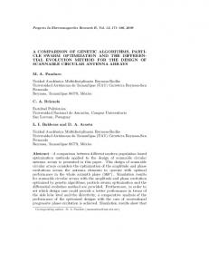
A. A Simple Client Server Architecture The simplest distributed client–server architecture is shown in Figure 1. The servers have no local memory, do not communicate among themselves or store data locally or on a global and shared device. The client sends the individuals’ encodings to the servers and waits for the fitness values to be returned. Each server has only its own local LSI matrix and computes fitness values based on the equations presented in the previous section. B. A Database Client Server Architecture Figure 2 shows the architecture of a client–server in which a database server stores global shared storage device. When a segment cohesion or coupling value is required, a server
first queries the database before computing it if missing. The database holds two tables: a cohesion table and a coupling table, each with three columns. Each record in these tables keeps a similarity/coupling value for one segment. The first column, called beginning, keeps the index of the first method invocation in a segment and the second column keeps the index of the last method invocation in the same segment. The third column contains the cohesion/coupling value of that segment. Whenever the fitness value for a new individual must be computed, the responsible server checks first the database. If it can find the needed values (already calculated in the last iterations or by other servers for other individuals), it uses these to compute the fitness value using a simple division. Else, it computes cohesion and coupling for the new segment and stores the values in the database. Thus, computation is performed if and only if the values can not be retrieved from the database: as much data as possible is shared between servers to reduce computation times. There is an extra cost due to database queries and network communication. A central database implies that all servers write in and read from the same database. Yet, we would expected that using a database reduces the computation times by caching already-calculated values. However, sending data over the network, acquiring and releasing locks, and performing queries are also time consuming operations. C. A Hash-database Client Server Architecture To limit the possible communication between servers and the database, the architecture shown in Figure 3 was devised.
The goal of this architecture is to further reduce computation time by decreasing the number of accesses to the central database using a local cache on each server, implemented with a hash table. The architecture works as follows: whenever a server wants to compute the fitness value of a segment, it searches its hash table. If the required data does not exist in its local hash table, then the server queries the central database. If the server finds the required data in the database, it uses it to compute the fitness value and and stores it in its hash table, else it computes the required data and stores the results in both its hash table for its future use and in the central database for the other servers use. Figure 4 reports the flowchart of the process of this architecture. D. A Hash Client Server Architecture This last architecture is a compromise between the two previous ones: only local data is stored in the local hash table of servers. No data is shared among servers. As shown in Figure 5, servers only communicate with the client and no global data is kept and available. Each server has two hash tables: one for similarity cohesion and the other for coupling values for each segment. The key of the hash tables is a combination of the indexes of the first and last method invocations of a segment. Each server uses its own hash tables and thus cannot benefit from the computation results of others. However, because all the data is stored locally and there is no access policy using locking algorithms, the access to the already-calculated data as well as their storage is efficient. V. R ESULTS AND D ISCUSSION We now report the typical timing obtained with the different architectures on two compressed traces from JHotDraw. JHotDraw3 is a Java framework for drawing 2D graphics. JHotDraw started in October 2000 with the main purpose of illustrating the use of design patterns in a real context. Version v5.4b2 used in our previous work [14] has a size of about 413 KLOCs. The traces were collected by instrumenting JHotDraw and executing the scenarios Start-DrawRectangle-Quit and StartSpawn-Window-Draw-Circle-Stop. These scenarios generated respectively traces of 6,668 and 16,366 method calls; once utility methods were removed their sizes are reduced to 447 and 670 calls. Finally RLE compression brought down the numbers of distinct calls to 240 and 432. In our experiments, we distributed computations over a sub-network of 14 workstations. Five high-end workstations, the most powerful ones, are connected in a Gigabit Ethernet LAN; low-end workstations are connected to a LAN segment at 100 MBit/s and talk among themselves at 100 Mbit/s. Each experience was run on a subset of ten computers: nine servers and one client. 3 http://www.jhotdraw.org
Workstations run CentOS v5 64 bits; memory varies between four to 16 Gbytes. Workstations are based on Athlon X2 Dual Core Processor 4400; the five high-end workstations are either single or dual Opteron. Workstations run basic Unix services (e.g., network file system, SAMBA, mySQL) and user processes. User processes are typically editing and compilation of programs, e-mail clients, Web browsers, and so on. No special care was taken to ensure a specific network condition (e.g., priorities were not altered) and thus times and ratios between times can be considered typical of a industrial or research environment. However, the sizes of the GA processes never exceeded the physical memory of the workstations to avoid paging; workstations were managed to ensure that each computationally-intensive user processes had a dedicated CPU. The client computer was also responsible to measure execution times and to verify the liveness of connections; connections to servers as well as connections to the database were implemented on top of TCP/IP (AF INET) sockets. All components have been implemented in Java 1.5 64bits. The database server, shown in Figures 2 and 3, was MySQL server v5.0.77. Table III C OMPUTATION TIMES FOR DESKTOP SOLUTION AND THE DIFFERENT ARCHITECTURES OF F IGURES 1, 2, AND 5 WITH THE Start-DrawRectangle-Quit SCENARIO – C OMPRESSED TRACE LENGTH OF 240 METHODS Time Measurement Runs # Measures 1 12:09 h 2 11:39 h Desktop 3 12:21 h 4 11:50 h 5 12:38 h 1 1:44 h 2 2:36 h Client–server 3 1:53 h 4 1:40 h 5 2:13 h 1 16:36 h Database 2 15:3 h 3 9:52 h 1 5:13 m 2 5:19 m Hash Table 3 5:20 m 4 5:27 m 5 5:10 m Architectures
Average
12:07 h
2:01 h
13:50 h
5:17 m
Table III reports computation times for the different architectures. The times reported for the single-computer architecture come from an optimized implementation of our approach. In our first implementation, we reused the Java GALib library, which is freely available from SourceForge and implements a simple GA. GALib makes no assumptions on crossover and mutation operators and assumes that the fitness of an individual must be recomputed even if it was passed unchanged from the old generation to the new one. This recomputation resulted in about 30% of computationtime increase because between 20% and 30% of individuals
Table IV C OMPUTATION TIMES FOR DESKTOP SOLUTION AND THE ARCHITECTURE OF F IGURE 5 WITH THE Start-Spawn-Window-Draw-Circle-Stop SCENARIO – C OMPRESSED TRACE LENGTH OF 432 METHODS
Architectures Desktop
Hash Table
Time Measurement Runs # Measures 1 45:38 h 2 41:28 h 3 45:07h 1 7:21 m 2 7:21 m 3 7:32 m
Average 44:07
7:24 m
are not subject to mutation or crossover between generations. Thus, to reduce computation time, we modified GALib to compute only the fitness values of individuals that have changed between the last generation and the current one. Distributing the computation, shown in Figure 1, clearly results in an important reduction of computation time; as shown in the second row of Table III. Computation time went from 12 hours to about two hours; however, the gain in terms of time reduction is considerably lower than expected as we had nine computers available (excluding the client) and, thus, expected computation times close to one hour. We felt that there was still room for improvement and Amdahl’s law [40] was only partially the reason for the reduced gain. We observed that the nature of our problem was such that crossover and mutation preserve a large fraction of segments unchanged and that for those segments, previous cohesion and coupling values could be reused. Thus, we tested the two architectures in Figures 2 and 3. Table III in its third row reports results for such database client–server architecture: to our surprise, sharing data among servers via a central database increased computation times. Finally, Table III, in its last row, reports the computation times for the architecture in Figure 5, which is the fastest architectures. The gain in computation times obtained is of about 140 times. The implementation of this GA parallelization is moreover relatively simple. We obtained similar gains with other traces. For example, the trace generated by the scenario Start-Spawn-WindowDraw-Circle-Stop, with the desktop architecture, was split in about 44 hours while, with the fastest architecture, the client–server with the hash table, computation time is of about 7 minutes. Table IV reports the results of splitting the trace with two architectures. A. Discussion We conjecture that poor performance of the database architecture, in Figure 2, is mainly due to the database accesses (reading, writing, and locking) for the computation of each coupling and cohesion values. These frequent accesses are responsible for the increase in computation times. To limit
the number of database accesses, we introduced the hybrid architecture in Figure 3. Results have not been reported in Table III because they are not substantially different (better) then those of the database. We are investigating the reason of this unexpected behavior to locate the bottleneck cause. Indeed, in our current implementation, accesses to the local hash table and the database are managed serially. Performance could improve by parallelizing writing in the database and access to the hash table and by loading the hash table only once at the beginning of each computation. Unfortunately, given the size of the search space and the huge number of possible segments, the probability that in two consecutive runs a relevant number of the segments will be exactly the same is very low. This fact makes the architecture in Figure 3 interesting from a theoretical point of view but not practical. Despite the decrease in computation time, the very definition of the concept location problem makes it hard to obtain acceptable computation times for traces longer than few thousands of methods even with the fastest architecture, unless a higher number of servers is available. The definition of this problem is tied to the size of the search space, Equations 1 and 2, and the bit-string representation. Indeed, the longer the trace, the higher the number of methods contributing to the segment coupling. However, we believe that if concepts are indeed implemented in cohesive and decoupled segments, then computing coupling with Equation 2 is overly conservative and redefining the problem could substantially reduce computation time. We are currently working to restate the concept location problem in using audio digital signal processing and time windowing. We have reported data of two traces of one software system, namely JHotDraw, therefore we cannot generalize to other traces though the performance issue is likely to be non-specific to JHotDraw or the used traces. Indeed, we experienced similar results with traces of different lengths of ArgoUML. Much in the same way, we cannot generalize to other search-based software engineering problems. However, we observed that the trade-off between the complexity of the fitness function and the local and global knowledge representations; similar trade-offs are known to be general and common to many application of optimization techniques to software engineering. VI. C ONCLUSION AND F UTURE W ORK GAs have been successfully applied to many complex software engineering problems. To the best of our knowledge, no previous work distributed fitness computation on several servers to exploit the intrinsic parallel nature of GAs to reduce computation times for concept location. This paper presented and discussed four client–server architectures conceived to improve performance and reduce GA computation times to resolve the concept location problem. To our surprise, we discovered that on a standard
TCP/IP network, the overhead of database accesses, communication, and latency may impair a dedicated solutions. Indeed, in our experiments, the fastest solution was an architecture where each server kept track only of its computations without exchanging data with other servers. This simple architecture reduced GA computation by about 140 times when compared to a simple implementation, in which all GA operations are performed on a single machine. Future work will follow different directions. First, we are working on reformulating the concept location problem. Also, we want to experiment different communication protocols (e.g., UDP) and synchronization strategies. We will carry out other empirical studies to evaluate the approach on more traces, obtained from different systems, to verify the generality of our findings. Finally, we will reformulate other search-based software engineering problems to exploit parallel computation to verify further our findings. VII. ACKNOWLEDGEMENTS This research was partially supported by the Natural Sciences and Engineering Research Council of Canada (Research Chair in Software Evolution and in Software Patterns and Patterns of Software) and by G. Antoniol’s Individual Discovery Grant. R EFERENCES [1] M. Garey and D. Johnson, Computers and Intractability: a Guide to the Theory of NP-Completeness. W.H. Freeman, 1979. [2] G. Antoniol and M. D. Penta, “Library miniaturization using static and dynamic information,” in Proceedings of IEEE International Conference on Software Maintenance. Amsterdam The Netherlands: IEEE Press, Sep 22-26 2003, pp. 235–244. [3] G. Antoniol, A. Cimitile, A. D. Lucca, and M. D. Penta, “Assessing staffing needs for a software maintenance project through queuing simulation,” IEEE Transactions on Software Engineering, vol. 30, no. 1, pp. 43–58, Jan 2004.
[9] G. Antoniol and Y.-G. Gu´eh´eneuc, “Feature identification: An epidemiological metaphor,” Transactions on Software Engineering (TSE), vol. 32, no. 9, pp. 627–641, September 2006, 15 pages. [10] T. Biggerstaff, B. Mitbander, and D. Webster, “The concept assignment problem in program understanding,” in Proceedings of the International Conference on Software Engineering, IEEE Computer Society Press, May 1993, pp. 482–498. [11] V. Kozaczynski, J. Q. Ning, and A. Engberts, “Program concept recognition and transformation,” IEEE Transactions on Software Engineering, vol. 18, no. 12, pp. 1065–1075, Dec 1992. [12] Denys Poshyvanyk, Y.-G. Gu´eh´eneuc, A. Marcus, G. Antoniol, and V. Rajlich, “Feature location using probabilistic ranking of methods based on execution scenarios and information retrieval,” Transactions on Software Engineering (TSE), vol. 33, no. 6, pp. 420–432, June 2007, 14 pages. [13] P. Tonella and M. Ceccato, “Aspect mining through the formal concept analysis of execution traces,” in Proceedings of IEEE Working Conference on Reverse Engineering, 2004, pp. 112– 121. [14] F. Asadi, M. D. Penta, G. Antoniol, and Y.-G. Gueheneuc, “A heuristic-based approach to identify concepts in execution traces,” in European Conference on Software Maintenance and Reengineering, Madrid (Spain), Mar 15-18 2010, pp. 31– 40. [15] A. Nicolas and L. Timothy, “Extracting concepts from file names; a new file clustering criterion,” in Proceedings of the International Conference on Software Engineering, April 1998, pp. 84–93. [16] N. Wilde and M. Scully, “Software reconnaissance: Mapping program features to code,” Journal of Software Maintenance - Research and Practice, vol. 7, no. 1, pp. 49–62, Jan 1995. [17] M. Eaddy, A. Aho, G. Antoniol, and Y.-G. Gueheneuc, “Cerberus: Tracing requirements to source code using information retrieval dynamic analysis and program analysis,” in ICPC ’08: Proceedings of the 2008 The 16th IEEE International Conference on Program Comprehension. Washington DC USA: IEEE Computer Society, 2008, pp. 53–62.
[4] P. McMinn and M. Holcombe, “Evolutionary testing using an extended chaining approach,” Evol. Comput., vol. 14, no. 1, pp. 41–64, 2006.
[18] W. E. Wong, S. S. Gokhale, and J. R. Horgan, “Quantifying the closeness between program components and features,” Journal of Systems and Software, vol. 54, no. 2, pp. 87 – 98, 2000, special Issue on Software Maintenance.
[5] M. O’Keeffe and M. O. Cinn´eide, “Search-based refactoring: an empirical study,” J. Softw. Maint. Evol., vol. 20, no. 5, pp. 345–364, 2008.
[19] D. Edwards, S. Simmons, and N. Wilde, “An approach to feature location in distributed systems,” Software Engineering Research Center, Tech. Rep., 2004.
[6] J. Stender, Parallel Genetic Algorithm: Theory and Applications, 1993, vol. 14 Frontiers in Artificial Intelligence and Applications.
[20] A. D. Eisenberg and K. D. Volder, “Dynamic feature traces: Finding features in unfamiliar code,” in proceedings of the 21s t International Conference on Software Maintenance. IEEE Press, September 2005, pp. 337–346.
[7] W. Rivera, “Scalable parallel genetic algorithms,” Artif. Intell. Rev., vol. 16, no. 2, pp. 153–168, 2001. [8] E. Alba, Parallel Metaheuristics. John Wiley and Sons Inc, 2005.
[21] N. Gold, M. Harman, Z. Li, and K. Mahdavi, “Allowing overlapping boundaries in source code using a search based approach to concept binding,” Proceedings of the 22nd IEEE International Conference on Software Maintenance (ICSM ’06), pp. 310–319, 2006.
[22] N. Gold, “Hypothesis-based concept assignment to support software maintenance,” 17th IEEE International Conference on Software Maintenance (ICSM’01), pp. 545–548, 2001. [23] L. Dapeng, M. Andrian, P. Denys, and R. Vaclav, “Feature location via information retrieval based filtering of a single scenario execution trace,” in ASE ’07: Proceedings of the twenty-second IEEE/ACM international conference on Automated software engineering. New York NY USA: ACM, 2007, pp. 234–243. [24] A. Marcus, D. Poshyvanyk, and R. Ferenc, “Using the conceptual cohesion of classes for fault prediction in objectoriented systems,” IEEE Transactions on Software Engineering, vol. 34, no. 2, pp. 287–300, 2008. [25] D. Poshyvanyk and A. Marcus, “The conceptual coupling metrics for object-oriented systems,” in Proceedings of 22nd IEEE International Conference on Software Maintenance. Philadelphia Pennsylvania USA: IEEE CS Press, 2006, pp. 469 – 478. [26] B. S. Mitchell, M. Traverso, and S. Mancoridis, “An architecture for distributing the computation of software clustering algorithms,” Proceedings of the Working IEEE/IFIP Conference on Software Architecture (WICSA ’01), pp. 181–190, 2001. [27] K. Mahdavi, M. Harman, and R. M. Hierons, “A multiple hill climbing approach to software module clustering,” Proceedings of the International Conference on Software Maintenance (ICSM ’03), pp. 315–324, 2003. [28] S. Yussof, R. A. Razali, and O. H. See, “A parallel genetic algorithm for shortest path routing problem,” Proceedings of the 2009 International Conference on Future Computer and Communication, pp. 268–273, 2009. [29] W. Zhi-xin and J. Gang, “A parallel genetic algorithm in multi-objective optimization,” Control and Decision Conference, 2009. CCDC ’09. Chinese, pp. 3497–3501, 2009. [30] F. Liu, X. Chen, and Z. Huang, “Parallel genetic algorithm for finding roots of complex functional equation,” 2nd International Conference on Pervasive Computing and Applications, 2007. ICPCA, pp. 542–545, 2007. [31] Y.-W. Chen, Z. Nakao, and X. Fang, “A parallel genetic algorithm based on the island model for image restoration,” Proceedings of the 1996 IEEE Signal Processing Society Workshop on Neural Networks for Signal Processing [1996] VI., pp. 109 – 118, 1996. [32] Y. Fukuyama and H.-D. Chiang, “A parallel genetic algorithm for service restoration in electric power distribution systems,” In Proceedings of the 1995 IEEE International Conference on Fuzzy Systems, pp. 275–282, 1995. [33] D. L. A. de Araujo, H. S. Lopes, and A. A. Freitas, “A parallel genetic algorithm for rule discovery in large databases,” 1999 IEEE International Conference on Systems, Man, and Cybernetics, 1999 (IEEE SMC99), vol. 3, pp. 940–945, 1999.
[34] B. Zorman, G. M. Kapfhammer, and R. Roos, “Creation and analysis of a javaspace-based distributed genetic algorithm,” Proceedings of the International Conference on Parallel and Distributed Processing Techniques and Applications, vol. 3, pp. 1107 – 1112, 2002. [35] Janice Ka-Yee Ng, Y.-G. Gu´eh´eneuc, and G. Antoniol, “Identification of behavioral and creational design motifs through dynamic analysis,” Journal of Software Maintenance and Evolution: Research and Practice (JSME), December 2009, under publication. [36] M. F. Porter, “An algorithm for suffix stripping,” Program, vol. 14, no. 3, pp. 130–137, 1980. [37] R. Baeza-Yates and B. Ribeiro-Neto, Modern Information Retrieval. Addison-Wesley, 1999. [38] S. Deerwester, S. T. Dumais, G. W. Furnas, T. K. Landauer, and R. Harshman, “Indexing by latent semantic analysis,” Journal of the American Society for Information Science, vol. 41, no. 6, pp. 391–407, 1990. [39] B. S. Mitchell and S. Mancoridis, “On the automatic modularization of software systems using the bunch tool.” IEEE Trans. Software Eng., vol. 32, no. 3, pp. 193–208, 2006. [40] G. M. Amdahl, “Validity of the single processor approach to achieving large scale computing capabilities,” in AFIPS ’67: Proceedings of the spring joint computer conference. New York, NY, USA: ACM, 1967, pp. 483–485. [41] D. Garlan and M. Shaw, “An introduction to software architecture,” in Advances in Software Engineering and Knowledge Engineering, vol. 1. New York: World Scientific, 1993.