Using Genetic Algorithms for Concept Learning - CiteSeerX

Using Genetic Algorithms for Concept Learning

Kenneth A. De Jong, William M. Spears and Diana F. Gordon Naval Research Laboratory Washington, D.C. 20375 and George Mason University Fairfax, VA 22030

Abstract In this paper, we explore the use of genetic algorithms (GAs) as a key element in the design and implementation of robust concept learning systems. We describe and evaluate a GA-based system called GABIL that continually learns and refines concept classification rules from its interaction with the environment. The use of GAs is motivated by recent studies showing the effects of various forms of bias built into different concept learning systems, resulting in systems that perform well on certain concept classes (generally, those well matched to the biases) and poorly on others. By incorporating a GA as the underlying adaptive search mechanism, we are able to construct a concept learning system that has a simple, unified architecture with several important features. First, the system is surprisingly robust even with minimal bias. Second, the system can be easily extended to incorporate traditional forms of bias found in other concept learning systems. Finally, the architecture of the system encourages explicit representation of such biases and, as a result, provides for an important additional feature: the ability to dynamically adjust system bias. The viability of this approach is illustrated by comparing the performance of GABIL with that of four other more traditional concept learners (AQ14, C4.5, ID5R, and IACL) on a variety of target concepts. We conclude with some observations about the merits of this approach and about possible extensions. Key words: concept learning, genetic algorithms, bias adjustment

-21. Introduction An important requirement for both natural and artificial organisms is the ability to acquire concept classification rules from interactions with their environment. In this paper, we explore the use of an adaptive search technique, namely, genetic algorithms (GAs), as the central mechanism for designing such systems. The motivation for this approach comes from an accumulating body of evidence that suggests that, although concept learners require fairly strong biases to induce classification rules efficiently, no a priori set of biases is appropriate for all concept learning tasks. We have been exploring the design and implementation of more robust concept learning systems which are capable of adaptively shifting their biases when appropriate. What we find particularly intriguing is the natural way GA-based concept learners can provide this capability. As proof of concept we have implemented a system called GABIL with these features and have compared its performance with four more traditional concept learning systems (AQ14, C4.5, ID5R, and IACL) on a set of target concepts of varying complexity. We present these results in the following manner. We begin by showing how concept learning tasks can be represented and solved by traditional GAs with minimal implicit bias. We illustrate this by explaining the GABIL system architecture in some detail. We then compare the performance of this minimalist GABIL system with AQ14, C4.5, ID5R, and IACL on a set of target concepts of varying complexity. As expected, no single system is best for all of the presented concepts. However, a posteriori one can identify the biases that were largely responsible for each system’s superiority on certain classes of target concepts. We then show how GABIL can be easily extended to include these biases, which improves system performance on various classes of concepts. However, the introduction of additional biases raises the problem of how and when to apply them to achieve the bias adjustment necessary for more robust performance. Finally, we show how a GA-based system can be extended to dynamically adjust its own bias in a very natural way. We support these claims with empirical studies showing the improvement in robustness of GABIL with adaptive bias, and we conclude with a discussion of the merits of this approach and directions for further research.

2. GAs and Concept Learning Supervised concept learning involves inducing descriptions (i.e., inductive hypotheses) for the concepts to be learned from a set of positive and negative examples of the target concepts. Examples (instances) are represented as points in an ndimensional feature space which is defined a priori and for which all the legal values of the features are known. Concepts are therefore represented as subsets of points in the given n-dimensional space. A concept learning program is presented with both a description of the feature space and a set of correctly classified examples of the concepts, and is expected to generate a reasonably accurate description of the (unknown) concepts.

-3The choice of the concept description language is important in several respects. It introduces a language bias which can make some classes of concepts easy to describe while other class descriptions become awkward and difficult. Most of the approaches have involved the use of classification rules, decision trees or, more recently, neural networks. Each such choice also defines a space of all possible concept descriptions from which the "correct" concept description must be selected using a given set of positive and negative examples as constraints. In each case the size and complexity of this search space requires fairly strong additional heuristic pruning in the form of biases towards concepts which are "simpler", "more general", and so on. The effects of adding such biases in addition to the language bias is to produce systems that work well on concepts that are well-matched to these biases, but perform poorly on other classes of concepts. What is needed is a means for improving the overall robustness and adaptability of these concept learners in order to successfully apply them to situations in which little is known a priori about the concepts to be learned. Since genetic algorithms (GAs) have been shown to be a powerful adaptive search technique for large, complex spaces in other contexts, our motivation for this work is to explore their usefulness in building more flexible and effective concept learners. 1 In order to apply GAs to a concept learning problem, we need to select an internal representation of the space to be searched. This must be done carefully to preserve the properties that make the GAs effective adaptive search procedures (see (DeJong, 1987) for a more detailed discussion). The traditional internal representation of GAs involves using fixed-length (generally binary) strings to represent points in the space to be searched. However, such representations do not appear well-suited for representing the space of concept descriptions that are generally symbolic in nature, that have both syntactic and semantic constraints, and that can be of widely varying length and complexity. There are two general approaches one might take to resolve this issue. The first involves changing the fundamental GA operators (crossover and mutation) to work effectively with complex non-string objects. Alternatively, one can attempt to construct a string representation that minimizes any changes to the GA. Each approach has certain advantages and disadvantages. Developing new GA operators which are sensitive to the syntax and semantics of symbolic concept descriptions is appealing and can be quite effective, but also introduces a new set of issues relating to the precise form such operators should take and the frequency with which they should be applied. The alternative approach, using a string representation, puts the burden on the system designer to find a mapping of complex concept descriptions into linear strings which has the property that the traditional GA operators that manipulate these strings preserve the syntax and semantics of the underlying concept descriptions. The advantage of this approach is that, if an effective mapping can be defined, a standard "off the shelf" GA can be used with few, if any, changes. In this paper, we illustrate the latter approach and develop a system which uses a traditional GA with minimal changes. For examples of the other approach see (Rendell, 1985; Grefenstette, 1989; Koza, 1991; Janikow, 1991). The decision to adopt a minimalist approach has immediate implications for the choice of concept description languages. We need to identify a language that can be _______________ 1

Excellent introductions to GAs can be found in (Holland, 1975) and (Goldberg, 1989).

-4effectively mapped into string representations and yet retains the necessary expressive power to represent complex concept descriptions efficiently. As a consequence, we have chosen a simple, yet general rule language for describing concepts, the details of which are presented in the following sections.

2.1. Representing the search space A natural way to express complex concepts is as a disjunctive set of possibly overlapping classification rules, i.e., in disjunctive normal form (DNF). The left-hand side of each rule (i.e., disjunct or term) consists of a conjunction of one or more tests involving feature values. The right-hand side of a rule indicates the concept (classification) to be assigned to the examples that are matched (covered) by the left-hand side of the rule. Collectively, a set of such rules can be thought of as representing the unknown concept if the rules correctly classify the elements of the feature space. If we allow arbitrarily complex terms in the conjunctive left-hand side of such rules, we will have a very powerful description language that will be difficult to represent as strings. However, by restricting the complexity of the elements of the conjunctions, we are able to use a string representation and standard GAs, with the only negative side effect that more rules may be required to express the concept. This is achieved by restricting each element of a conjunction to be a test of the form: If the value of feature i of the example is in the given value set, return true else, return false. For example, a rule might take the following symbolic form: If (F1 = large) and (F2 = sphere or cube) then it is a widget. Since the left-hand sides are conjunctive forms with internal disjunction (e.g., the disjunction within feature F2), there is no loss of generality by requiring that there be at most one test for each feature (on the left hand side of a rule). The result is a modified DNF that allows internal disjunction. (See (Michalski, 1983) for a discussion of internal disjunction.) With these restrictions we can now construct a fixed-length internal representation for classification rules. Each fixed-length rule will have N feature tests, one for each feature. Each feature test will be represented by a fixed-length binary string, the length of which will depend on the type of feature (nominal, ordered, etc.). Currently, GABIL only uses features with nominal values. The system uses k bits for the k values of a nominal feature. So, for example, if the set of legal values for feature F1 is {small, medium, large}, then the pattern 011 would represent the test for F1 being medium or large. Further suppose that feature F2 has the values {sphere, cube, brick, tube} and there are two classes, widgets and gadgets. Then, a rule for this 2 feature problem would be represented internally as:

-5-

F1 F2 Class 111 1000 0 This rule is equivalent to: If (F1 = small or medium or large) and (F2 = sphere) then it is a widget. Notice that a feature test involving all 1s matches any value of a feature and is equivalent to "dropping" that conjunctive term (i.e., the feature is irrelevant for that rule). So, in the example above, only the values of F2 are relevant and the rule is more succinctly interpreted as: If (F2 = sphere) then it is a widget. For completeness, we allow patterns of all 0s which match nothing. This means that any rule containing such a pattern will not match any points in the feature space. While rules of this form are of no use in the final concept description, they are quite useful as storage areas for GAs when evolving and testing sets of rules. The right-hand side of a rule is simply the class (concept) to which the example belongs. This means that our rule language defines a "stimulus-response" system with no message passing or any other form of internal memory such as those found in (Holland, 1986). In many of the traditional concept learning contexts, there is only a single concept to be learned. In these situations there is no need for the rules to have an explicit right-hand side, since the class is implied. Clearly, the string representation we have chosen handles such cases easily by assigning no bits for the right-hand side of each rule.

2.1.1. Sets of classification rules Since a concept description will consist of one or more classification rules, we still need to specify how GAs will be used to evolve sets of rules. There are currently two basic strategies: the Michigan approach exemplified by Holland’s classifier system (Holland, 1986), and the Pittsburgh approach exemplified by Smith’s LS-1 system (Smith, 1983). Systems using the Michigan approach maintain a population of individual rules that compete with each other for space and priority in the population. In contrast, systems using the Pittsburgh approach maintain a population of variable-length rule sets that compete with each other with respect to performance on the domain task. There is still much to be learned about the relative merits of the two approaches. In this paper we report on results obtained from using the Pittsburgh approach.2 That is, each individual in the population is a variable-length string representing an unordered set of fixed-length _______________ 2 (Greene & Smith, 1987) and (Janikow, 1991) have also used the Pittsburgh approach. See (Wilson, 1987) and (Booker, 1989) for examples of the Michigan approach.

-6rules. The number of rules in a particular individual can be unrestricted or limited by a user-defined upper bound. To illustrate this representation more concretely, consider the following example of a rule set with 2 rules: F1 F2 Class 100 1111 0

F1 F2 Class 011 0010 0

This rule set is equivalent to: If (F1 = small) then it is a widget. or If ((F1 = medium or large) and (F2 = brick)) then it is a widget. 2.1.2. Rule Set Execution Semantics In choosing a rule set representation for use with GAs, it is also important to define simple execution semantics which encourage the development of rule subsets and their subsequent recombination with other subsets to form new and better rule sets. One important feature with this property is that there is no order-dependency among the rules in a rule set. When a rule set is used to predict the class of an example, the left-hand sides of all rules in a rule set are checked to see if they match (cover) a particular example. This "parallel" execution semantics means that rules perform in a locationindependent manner. It is possible that an example might be covered by more than one rule. There are a number of existing approaches for resolving such conflicts on the basis of dynamically calculated rule strengths, by measuring the complexity of the left-hand sides of rules, or by various voting schemes. It is also possible that there are no rules that cover a particular example. Unmatched examples could be handled by partial matching and/or covering operators. How best to handle these two situations in the general context of learning multiple concepts (classes) simultaneously is a difficult issue which we have not yet resolved to our satisfaction. However, these issues are considerably simpler when learning single concepts. In this case it is quite natural to view the rules in a rule set as a union of (possibly overlapping) covers of the concept to be learned. Hence, an example which matches one or more rules is classified as a positive example of the concept, and an example which fails to match any rule is classified as a negative example. In this paper, we focus on the simpler case of single-concept learning problems (which have also dominated the concept-learning literature). We have left the extension to multi-concept problems for future work.

-72.1.3. Crossover and mutation Genetic operators modify individuals within a population to produce new individuals for testing and evaluation. Historically, crossover and mutation have been the most important and best understood genetic operators. Crossover takes two individuals and produces two new individuals, by swapping portions of genetic material (e.g., bits). Mutation simply flips random bits within the population, with a small probability (e.g., 1 bit per 1000). One of our goals was to achieve a concept learning representation that could exploit these fundamental operators. We feel we have achieved that goal with the variable-length string representation involving fixed-length rules described in the previous sections. Our mutation operator is identical to the standard one and performs the usual bitlevel mutations. We are currently using a fairly standard extension of the traditional 2point crossover operator in order to handle variable-length rule sets. 3 With standard 2point crossover on fixed-length strings, there are only two degrees of freedom in selecting the crossover points since the crossover points always match up on both parents (e.g., exchanging the segments from positions 12-25 on each parent). However, with variable length strings there are four degrees of freedom since there is no guarantee that, having picked two crossover points for the first parent, the same points exist on the second parent. Hence, a second set of crossover points must be selected for it. As with standard crossover, there are no restrictions on where the crossover points may occur (i.e., both on rule boundaries and within rules). The only requirement is that the corresponding crossover points on the two parents "match up semantically". That is, if one parent is being cut on a rule boundary, then the other parent must be cut on a rule boundary. Similarly, if one parent is being cut at a point 5 bits to the right of a rule boundary, then the other parent must be cut in a similar spot (i.e., 5 bits to the right of some rule boundary). For example consider the following two rule sets: F1

F2

Class

F1 F2

Class

10|0 0100| 0 011 0010 0 | | | ------------------------| | 01|0 0001 0 110 0011| 0 We use a "|" to denote a crossover cut point. Note that the left cut point is offset 2 bits from the rule boundary, while the right cut point is offset 1 bit from the rule boundary. The bits within the cut points are swapped, resulting in a rule set of 3 rules and a rule set of 1 rule: _______________ 3

We are also investigating the use of a uniform crossover operator that has been recently shown to be more effective in certain contexts than 2-point crossover.

-8-

F1 F2

Class F1 F2 Class F1 F2 Class

100 0001 0

110 0011 0

011 0010 0

010 0100 0

2.2. Choosing a fitness function In addition to selecting a good representation, it is important to define a good fitness function that rewards the right kinds of individuals. In keeping with our minimalist philosophy, we selected a fitness function involving only classification performance (ignoring, for example, length and complexity biases). The fitness of each individual rule set is computed by testing the rule set on the current set of training examples (which is typically a subset of all the examples - see Section 2.6) and letting: fitness (individual i) = (percent correct )2 This provides a bias toward correctly classifying all the examples while providing a non-linear differential reward for imperfect rule sets. This bias is equivalent to one that encourages consistency and completeness of the rule sets with respect to the training examples. A rule set is consistent when it covers no negative examples and is complete when it covers all positive examples.

2.3. GABIL: A GA-based concept learner We are now in a position to describe GABIL, our GA-based concept learner. At the heart of this system is a GA for searching the space of rule sets for ones that perform well on a given set of positive and negative examples. Figure 1 provides a pseudo-code description of the GA used. -----------------------------------------------------------------------Insert Figure 1 about here -----------------------------------------------------------------------P(t) represents a population of rule sets. After a random initialization of the population, each rule set is evaluated with the fitness function described in section 2.2. Rule sets are probabilistically selected for survival in proportion to their fitness (i.e., how consistent and complete they are). Crossover and mutation are then applied probabilistically to the surviving rule sets, to produce a new population. This cycle continues until as consistent and complete a rule set as possible has been found within the time/space constraints given. Traditional concept learners differ in the ways examples are presented. Many systems presume a batch mode, where all instances are presented to the system at once. Others work in an incremental mode, where one or a few of the instances are presented to the system at a time. In designing a GA-based concept learner, the simplest approach

-9involves using batch mode, in which a fixed set of training examples is presented and the GA must search the space of variable-length strings described above for a set of rules with high fitness (100% implies completeness and consistency on the training set). However, in many situations learning is a never-ending process in which new examples arrive incrementally as the learner explores its environment. The examples themselves can in general contain noise and are not carefully chosen by an outside agent. These are the kinds of problems that we are most interested in, and they imply that a concept learner must evolve concept descriptions incrementally from non-optimal and noisy instances. The simplest way to produce an incremental GA concept learner is as follows. The concept learner initially accepts a single example from a pool of examples and searches for as perfect a rule set as possible for this example within the time/space constraints given. This rule set is then used to predict the classification of the next example. If the prediction is incorrect, the GA is invoked (in batch mode) to evolve a new rule set using the two examples. If the prediction is correct, the example is simply stored with the previous example and the rule set remains unchanged. As each new additional instance is accepted, a prediction is made, and the GA is re-run in batch mode if the prediction is incorrect. We refer to this mode of operation as batch-incremental and we refer to the GA batch-incremental concept learner as GABIL. Although batch-incremental mode is more costly to run than batch, it provides a much more finely-grained measure of performance that is more appropriate for situations in which learning never stops. Rather than measure an algorithm’s performance using only a small training subset of the instances for learning, batch-incremental mode measures the performance of this algorithm over all available instances. Therefore, every instance acts as both a testing instance and then a training instance. Our ultimate goal is to achieve a pure incremental system which is capable of responding to even more complex situations such as when the environment itself is changing during the learning process. In this paper, however, we report on the performance of GABIL, our batch-incremental concept learner.

3. Empirical System Comparisons The experiments described in this section are designed to compare the predictive performance of GABIL and four other concept learners as a function of incremental increases in the size and complexity of the target concept.

3.1. The domains The experiments involve two domains: one artificial, and one natural. Domain 1, the artificial domain, was designed to reveal trends that relate system biases to incremental increases in target concept complexity. For this domain, we invented a 4 feature world in which each feature has 4 possible distinct values (i.e., there are 256 instances in this world).

- 10 Within Domain 1, we constructed a set of 12 target concepts. We varied the complexity of the 12 target concepts by increasing both the number of rules (disjuncts) and the number of relevant features (conjuncts) per rule required to correctly describe the concepts. The number of disjuncts ranged from 1 to 4, while the number of conjuncts ranged from 1 to 3. Each target concept is labeled as nDmC, where n is the number of disjuncts and m is the number of conjuncts (see Appendix 2 for the definition of these target concepts). For each of the target concepts, the complete set of 256 instances were labeled as positive or negative examples of the target concept. The 256 examples were randomly shuffled and then presented sequentially in batch-incremental mode. This procedure was repeated 10 times (trials) for each concept and learning algorithm pair. For Domain 2, we selected a natural domain to further test our conjectures about system biases. Domain 2 is a well-known natural database for diagnosing breast cancer (Michalski et. al., 1986). This database has descriptions of cases for 286 patients, and each case (instance) is described in terms of 9 features. There is a small amount of noise of unknown origin in the database manifested as cases with identical features but different classifications. The target concept is considerably more complex than any of the concepts in the nDmC world. For example, after seeing all 286 instances, the AQ14 system (also known as NEWGEM, described below) develops an inductive hypothesis having 25 disjuncts and an average of 4 conjuncts per disjunct. Since GABIL and ID5R can only handle nominals, and the breast cancer instances have features in the form of numeric intervals, we converted the breast cancer (BC) database to use nominal features. This conversion necessarily loses the inherent ordering information associated with numeric intervals. For example, the feature age is defined to have numeric interval values {10-19, 20-29, ..., 90-99} in the original database, and is represented as the set {A1, A2, ..., A9} of nominals in the converted database. When using the BC database, we again randomly shuffled the instances and averaged over 10 runs. It should be noted that all the problems in these two test domains are single-class problems. As discussed earlier, evaluating this approach on multi-class problems is part of our future plans.

3.2. The systems The performance of the GABIL system described in section 2.3 was evaluated on both domains. Standard GA settings of 0.6 for 2-pt crossover and 0.001 for mutation were used. The choice of population size was more difficult. With large, complex search spaces, larger population sizes are preferable, but generally require more computation time. With our unoptimized batch-incremental version of GABIL, we were able to use a population size of 1000 for the artificial domain. However, for the BC domain, a population size of 100 was used in order to keep the experimental computation time reasonable.4 _______________ 4 Our unoptimized batch-incremental version of GABIL is somewhat slower than C4.5, AQ, and IACL. It is substantially slower than ID5R. One should not conclude from this, however, that GA concept learners are inherently slower. See Janikow (1991) for details.

- 11 To better assess the GABIL system, four other concept learners were also evaluated on the target concept domains. We selected four systems to represent all four combinations of batch and incremental modes, and two popular hypothesis forms (DNF and decision trees). The chosen systems are AQ14 (Mozetic, 1985), which is based on the AQ algorithm described in (Michalski, 1983), C4.5 (Quinlan, unpublished), ID5R (Utgoff, 1988), and Iba’s Algorithm Concept Learner (IACL) (Gordon, 1990), which is based on Iba’s algorithm described in (Iba, 1979). AQ14 and IACL form modified DNF hypotheses. The C4.5 and ID5R systems are based on the ID algorithm described in (Quinlan, 1986), and form decision tree hypotheses. AQ14 and C4.5 are run in batchincremental mode since they are batch systems. ID5R and IACL are incremental. AQ14, like AQ, generates classification rules from instances using a beam search. This system maintains two sets of classification rules for each concept: one set, which we call the positive hypothesis, is for learning the target concept and the other set, which we call the negative hypothesis is for learning the negation of the target concept. (Note that GABIL currently uses only a positive hypothesis.) AQ14, like GABIL, generates classification rules in a modified DNF that allows internal disjunction of feature values. Internal disjunction allows fewer external disjuncts in the hypotheses. AQ14’s learning method guarantees that its inductive hypotheses will be consistent and complete with respect to all training examples. The learning method, called the Star Algorithm, generates a hypothesis for each class C. Potential rules for this hypothesis are formed from a randomly-chosen example, called a seed, by maximally generalizing the description of the seed without covering any examples of the wrong class. One rule is chosen from the set of potential rules, using a user-specified set of criteria, and this rule is added to the hypothesis for C. This procedure repeats to generate more rules for the hypothesis until all examples of class C are covered by the hypothesis. AQ14’s criteria for hypothesis preferences (biases) influences its learning behavior. This system’s performance depends on these criteria, as well as on other parameter settings. The particular parameter settings that we chose for AQ14 implement a preference for simpler inductive hypotheses, e.g., inductive hypotheses having shorter rules.5 C4.5 uses a decision tree representation rather than a rule representation for its inductive hypotheses. Each decision tree node is associated with an instance feature. Each node represents a test on the value of the feature. Arcs emanating from a feature node correspond to values of that feature. Each leaf node is associated with a classification (e.g., positive or negative if one concept is being learned). To view a decision tree as a positive DNF hypothesis, one would consider this hypothesis to be the disjunction of all paths (a conjunction of feature values) from the root to a positive leaf. The negative hypothesis is simply the disjunction of all paths from the root to a negative leaf. _______________ 5

The precise criteria used are: the positive and negative inductive hypotheses are allowed to intersect provided the intersection covers no instances, noisy examples are considered positive, the maximum beam width is set to 20, and the minimum number of features and values are preferred in each rule. Other settings, which have less impact on system performance, are left at default values.

- 12 An information theoretic measure biases the search through the space of decision trees. Trees are constructed by first selecting a root node, then the next level of nodes, and so on. Those tree nodes, or features, that minimize entropy and therefore maximize information gain are selected first. The result is a preference for simpler (i.e., shorter) decision trees. C4.5 does not require completeness or consistency. Two configurations of C4.5 are available: pruned and unpruned. Pruning is a process of further simplifying decision trees. This process, which occurs after the decision tree has been generated, consists of testing the tree on previously seen instances and replacing subtrees with leaves or branches whenever this replacement improves the classification accuracy.6 Pruning is designed for both tree simplification (which increases the simplicity preference) and for improved prediction accuracy. Since it was not obvious to us when either configuration is preferable, we used both versions in our experiments. ID5R learns with the same basic algorithm as C4.5. However, this system learns incrementally. Other than the incremental learning, ID5R’s biases are nearly identical to those of C4.5 unpruned. One minor difference is that, unlike C4.5, ID5R does not predict the class of a new instance when it cannot make a prediction, e.g., when the instance is not covered by the decision tree. We have modified ID5R to make a random prediction in this case.7 The fourth system to be compared with GABIL is IACL (Gordon, 1990), a system similar to AQ14. IACL is not as well-known as the other systems described above and, therefore, we describe it in slightly more detail. IACL maintains two DNF hypotheses, one for learning the target concept, and one for learning the negation of that concept. Internal disjunction is permitted, and consistency and completeness is required. Unlike AQ14, though, IACL learns incrementally and prefers hypotheses that are more specific (i.e., less general) rather than simpler. A merging process maintains completeness. The merging process incorporates each new instance not already covered by a hypothesis into the hypothesis of the same class as that instance by performing a small amount of generalization. This is done by forming new hypothesis rules using a most specific generalization (MSG) operator. From every rule in the hypotheses, IACL forms a new rule that has feature values equal to the most specific generalization of the feature values of the new instance and those of the original rule. Each new rule is kept only if it is consistent with previous instances. Otherwise, the original rule is kept instead. If the instance cannot merge with any existing rule of the hypothesis, a description of it is added as a new rule. When the features are nominals, as is the case for our experiments, the most specific generalization is the internal disjunction of the feature values of the rule and those of the new instance. For example, suppose the system receives its first instance, which is positive and is a small sphere. Then the initial positive hypothesis is: _______________ 6

The type of pruning in C4.5 is a variant of pessimistic pruning described in (Quinlan, 1987) that prunes a tree to either a subtree or a leaf node (Quinlan, personal communication). 7 ID5R, like GABIL, is a research tool and therefore does not handle some of the realistic data characteristics (e.g., missing feature values) that can be handled by sophisticated systems such as C4.5.

- 13 -

if ((F1 = small) and (F2 = sphere)) then it is a widget. If the second instance is a medium cube, and it is positive, the positive hypothesis becomes: if ((F1 = small or medium) and (F2 = sphere or cube)) then it is a widget Note that this new hypothesis matches medium spheres and small cubes, though they have not been seen yet. IACL’s splitting process maintains consistency. If the system incorrectly predicts the class of a new instance, the system uses previously saved instances to relearn the hypotheses correctly. Let us continue with our example to illustrate the splitting process. Suppose the system now receives a new negative example that is a medium sphere. The current positive hypothesis matches this example, thereby violating the consistency requirement. After the splitting process, the positive hypothesis becomes: if ((F1 = small) and (F2 = sphere)) then it is a widget or if ((F1 = medium) and (F2 = cube)) then it is a widget,

and the negative hypothesis is: if (F1 = medium) and (F2 = sphere) then it is not a widget. New instances can be merged with these rules to generalize the hypotheses whenever merging preserves consistency with respect to previous instances.

3.3. Performance criteria We feel that learning curves are an effective means for assessing performance in the context of incremental concept learning. In the experiments reported here, each curve represents an average performance over 10 independent trials for learning a single target concept. During each trial, we keep track of a small window of recent outcomes, counting the correct predictions within that window. The value of the curve at each time step represents the percent correct achieved over the most recent window of instances. A window size of 10 was used for the artificial domain and one of size 50 for the BC domain. The sizes were chosen experimentally to balance the need for capturing recent behavior and the desire to smooth short term variations in the learning curves. After generating learning curves for each target concept, we collapsed the information from these curves into two performance criteria. The first, called the prediction accuracy (PA) criterion, is the average over all values on a learning curve, from the

- 14 beginning to the end of learning a target concept. We distilled the learning curves into a single average value to simplify the presentation of our results. The second performance criterion, called convergence (C), is the number of instances seen before a 95% prediction accuracy is maintained. If a 95% prediction accuracy can not be achieved (e.g., on the BC database), then C is not defined. The finely-grained measure obtainable with batch-incremental and incremental modes facilitates this performance criterion as well. The criteria just described are local in the sense that they apply to a single target concept. For each local criterion there is a corresponding global criterion that considers all target concepts in a domain. The global prediction accuracy criterion is the average of the PA criteria values on every target concept within a domain. Likewise, the global convergence criterion is the average of the C criteria values on all the target concepts of a domain. Since the global criteria are based on far more data than the local criteria, we base most of our conclusions from the experiments on the former.

3.4. Results Table 1 shows the results of the PA and global PA (denoted ‘‘Average’’ in the tables) criteria for measuring the performance of all systems on the nDmC and BC target concepts, while Table 2 shows the results of applying the C and global C (denoted ‘‘Average’’ in the tables) criteria to measure performance on the nDmC concepts only (since no system achieves 95% prediction accuracy on the BC database). Although there are differences between Tables 1 and 2, the general trend is similar. From these tables we can see that AQ14 is the best performer overall. In particular, AQ14 is the top or close to the top performer on the nDmC concepts. This system does not, however, perform as well as the other systems on the BC target concept (except IACL). These results are due to the fact that AQ14, when using our chosen parameter settings, is a system that is well tuned to simpler DNF target concepts.8 -----------------------------------------------------------------------Insert Table 1 about here ----------------------------------------------------------------------------------------------------------------------------------------------Insert Table 2 about here -----------------------------------------------------------------------IACL does not perform as well as the other systems on the BC target concept. We consider this to be a result of IACL’s sensitivity to our conversion of numeric intervals to nominals (as discussed earlier). IACL’s MSG operator is well-suited for learning when _______________ 8

AQ14 does not use flexible (partial) matching of hypotheses to instances. Flexible matching tends to improve the performance of the AQ systems (Michalski 1990). The newest version of AQ (AQTT-15), which uses flexible matching, was unavailable at the time of this study. In the future, we plan to run AQTT-15 on our suite of target concepts.

- 15 the instance features are structured nominals (i.e., have generalization trees to structure their values) or numeric, but is not well-suited for learning when the features are nominals. According to (Gordon, 1990), IACL performs very well on the numeric form of the BC database.9 Other experiments (not reported here) indicate that the conversion of the BC data to a nominal form does not adversely affect performance for AQ14 and C4.5. C4.5 pruned (abbreviated C4.5P in the tables) performs well on all but the target concepts that have many short disjuncts. On 4D1C, which has the most short disjuncts of any target concept in the artificial domain, all ID-based systems (C4.5 pruned and unpruned, as well as ID5R), perform poorly.10 Based on the global performance criteria, C4.5 unpruned (abbreviated C4.5U in the tables) performs the best of the ID-based systems on the artificial domain, whereas C4.5 pruned performs the best on the BC domain. GABIL appears to be a good overall performer. It does not do superbly on any particular concept, but it also does not have a distinct region of the space of concepts on which it clearly degrades. Furthermore, GABIL is quite competitive on the difficult BC target concept. The statistical significance of these results is presented in Appendix 1. It is clear from these results that none of the systems under evaluation is superior to all others on all the target concepts. The dominance of one technique on a certain class of concepts appears to be due in large part to the built-in forms of bias it embodies, and these can have a negative impact on other classes of concepts.

4. A More Robust Concept Learner The GABIL system evaluated above incorporates a "pure" GA as its search mechanism in the sense that there were no specific changes made to the internal representation or genetic operators relating to the task of concept learning. As in other application tasks, this generally results in a good overall GA-based problem solver, but one that can be outperformed by task-specific approaches particularly on simpler problems (see, for example, (De Jong & Spears, 1989)). However, one of the nice properties of a GA-based system is that it is not difficult to augment GAs with task-specific features to improve performance on that task. After obtaining the performance comparisons described in the previous section, we felt that extending GABIL with a small set of features appropriate to concept learning would significantly enhance its overall performance and robustness. Our approach was as follows. Each of the traditional concept learners evaluated above appeared to contain one or more biases that we considered to be largely responsible for that system’s success on a particular class of target concepts. We selected a subset of these biases to be implemented as additional "genetic" operators to be used by GABIL’s GA search procedure (see Figure 2). The virtue of this approach is the simple and unified way GABIL’s _______________ 9

When run in batch mode on the numeric BC database, with 70% of the instances in the training set and 30% in the test set, 72% of the predictions made on the test set were correct predictions (see Gordon, 1990). 10 An explanation of the difficulty of systems based on ID3 on target concepts of this type is in (De Jong & Spears, 1991).

- 16 underlying search process can be extended to include various traditional forms of concept learning bias. -----------------------------------------------------------------------Insert Figure 2 about here -----------------------------------------------------------------------Since AQ14 seemed to be the best overall performer, we selected it as our initial source of additional operators for GABIL. As we have described above, the AQ14 system used in our experiments has preferences for simpler and more general rules. After studying the results of our initial evaluation, we hypothesized that this is one of the biases largely responsible for AQ14’s superior performance on the nDmC concepts. This analysis led to the addition of two new GABIL operators which add biases for simpler and more general descriptions.

4.1. The adding alternative operator One of the mechanisms AQ uses to increase the generality of its inductive hypotheses is the "adding alternative" generalization operator of (Michalski, 1983). This operator generalizes by adding a disjunct (i.e., alternative) to the current classification rule. The most useful form of this operator, according to (Michalski, 1983), is the addition of an internal disjunct. For example, if the disjunct is (F1 = small) and (F2 = sphere) then the adding alternative operator might create the new disjunct (F1 = small) and (F2 = sphere or cube). This operator, which we call AA (the adding alternative operator), is easily implemented in GABIL by including an additional mutation that, unlike the normal mutation operator, has an asymmetric mutation rate. In particular, in the studies reported here, this operator incorporates a 75% probability of mutating a bit to a 1, but a 25% probability of mutating it to a 0. Therefore, the AA operator in GABIL has a strong preference for adding internal disjuncts. To illustrate, the adding alternative operator might change the disjunct F1 F2 100 100 to F1 F2 100 110

- 17 Note that feature F2 has been generalized in this disjunct. As with the other genetic operators, the adding alternative operator is applied probabilistically to a subset of the population each generation. In the studies reported here it was applied at a rate of 0.01 (1%). 11 For clarity in reporting the experimental results, we call the version of GABIL with the adding alternative operator ‘‘GABIL+A’’.

4.2. The dropping condition operator A second, and complementary, generalization mechanism leading to simpler hypotheses involves removing what appear to be nearly irrelevant conditions from a disjunct. This operator, which we call DC (the dropping condition operator), is based on the generalization operator of the same name described in (Michalski, 1983). For example, if the disjunct is (F1 = small or medium) and (F2 = sphere) then the DC operator might create the new disjunct (F2 = sphere). The DC operator is easily added to GABIL in the following manner. When this operator is applied to a particular member of the population (i.e., a particular rule set), each disjunct is deterministically checked for possible condition dropping. The decision to drop a condition is based on a criterion from (Gordon, 1990) and involves examining the bits of each feature in each disjunct. If more than half of the bits of a feature in a disjunct are 1s, then the remaining 0 bits are changed to 1s. By changing the feature to have all 1 values, this operator forces the feature to become irrelevant within that disjunct and thereby simulates the effect of a shortened disjunct. To illustrate, suppose this operator is applied to the following disjunct: F1 F2 110 100 Then the dropping condition operator will result in a new disjunct as follows: F1 F2 111 100 Note that feature F1 is now irrelevant within this disjunct. _______________ 11

Note that this is in addition to the standard mutation operator, which continues to fire with a probability of .001.

- 18 As with the other genetic operators, this new operator is applied probabilistically to a subset of the population each generation. In the experiments reported here, a rate of 0.60 (60%) was used. We make no claim that the rates used for either of these new operators are in any sense optimal. In these studies we selected a rate which seemed reasonable on the basis of a few informal experiments. Our preference (see section 5) is that such things be self-adaptive. We call GABIL with the DC operator ‘‘GABIL+D’’. When both task-specific operators are added to GABIL, the resulting system is called ‘‘GABIL+AD’’ (see Figure 3). Note that there is an interesting complementary relationship between these two operators in that adding alternatives can set the stage for dropping a condition altogether. -----------------------------------------------------------------------Insert Figure 3 about here -----------------------------------------------------------------------These augmented forms of GABIL do not change in any way the overall structure of the GA-based system described earlier (compare Figures 1 & 3). The only difference is that the set of "genetic" operators has been expanded. The result is that, after the traditional crossover and mutation operators have been used in the normal manner to produce new offspring (rule sets) from parents, the two new operators are (probabilistically) applied to each offspring, producing additional task-specific changes.

4.3. Results To study the effects of adding these bias operators to GABIL, GABIL+A, GABIL+D, and GABIL+AD have been run on the same concept domains used earlier. Table 3 shows the results of system performance measured using the PA and global PA criteria. Table 4 shows the results of system performance measured using the C and global C criteria. GABIL is abbreviated ‘‘G’’ in the tables. -----------------------------------------------------------------------Insert Table 3 about here ----------------------------------------------------------------------------------------------------------------------------------------------Insert Table 4 about here -----------------------------------------------------------------------According to the global criteria in Tables 3 and 4, GABIL+A does not perform as well as GABIL+D or GABIL+AD. On the BC target concept, the combination of both operators (GABIL+AD) is the best. It is interesting to note, however, that on the nDmC domain, GABIL+AD does not perform as well as GABIL+D. These results indicate that one can improve GABIL’s performance on certain classes of concepts by the addition of an appropriate set of bias operators. On the other

- 19 hand, it is not possible in general to know beforehand which set of biases is best. These results also point out the danger of indiscriminately including multiple biases as a strategy for overcoming this lack of a priori knowledge since multiple simultaneous biases can in fact interfere with one another, leading to a degradation in performance. These results, which confirm similar bias problems exhibited in other contexts, motivated us to focus on a more sophisticated way of improving GABIL’s overall robustness, namely, by having it dynamically adjust its own task-specific biases.

5. An Adaptive GA Concept Learner Although genetic algorithms themselves represent a robust adaptive search mechanism, most GA implementations involve static settings for such things as the population size, the kind of representation and operators used, and the operator probabilities. There have been a number of attempts to make these aspects of GAs more adaptive. We provide a brief overview of this work in the next section. 5.1. Adaptive GAs There have been two approaches to building more adaptive GAs, which we refer to as the within-problem approach and the across-problem approach. The within-problem approach adapts a GA dynamically, as it solves one problem. In contrast, the acrossproblem approach adapts GAs over the course of many problems. One good example of the across-problem approach is provided by (Grefenstette, 1986). In this paper, a separate meta-GA is used to adapt a GA as it solves a suite of problems. The advantage of such an approach is that the resulting system performs robustly on a suite of problems. Unfortunately, the approach is also time consuming, since each problem must be solved a large number of times. Furthermore, the adaptation is coarse, in the sense that the system is not necessarily optimal on any given problem. Within-problem adaptation provides a finer-grained approach, since the GA is adapted while one problem is solved. Furthermore, since the problem is solved only once, the approach can require much less time. We concentrate on the within-problem approach, since we wish to adapt the GA as it solves each concept learning problem. Within-problem approaches can be further divided into two categories, coupled and uncoupled, based on the observation that an adaptive GA is in effect searching two spaces: the original problem space, and the space of adaptations to the underlying GA itself. The relationship of these two search processes is an important design consideration for adaptive GAs. In a coupled approach, both searches are handled simultanously by a single GA search procedure. This is accomplished by using the underlying population to store information relevant to the adaptive mechanism as well as the standard information regarding the original problem space being searched. This approach is elegant and straightforward, since no new adaptive mechanism is required (see (Schaffer, 1987) for examples of this approach). Unfortunately, this coupling also means that the additional search can be hindered by the same issues that hinder the search of the problem space. For example, one possible concern is that this mechanism may only work well with large

- 20 population sizes. As with any other statistical sampling algorithm, small populations (samples) may be misleading and lead to wrong conclusions. This issue will be raised again later in this paper. An uncoupled approach does not rely upon the GA for the adaptive mechanism. Rather, the behavior of the underlying GA is adjusted by a separate control mechanism (see (Davis, 1989) and (Janikow, 1991) for examples). While this may alleviate the problems associated with coupling, such mechanisms appear to be difficult to construct, and involve complicated bookkeeping. Although we may explore this route in future work, we concentrate on the conceptually simpler coupled approach in this paper. We next consider how to implement a coupled within-problem approach within GABIL.

5.2. Adaptive GABIL Recall that the task-specific operators added to GABIL (DC and AA) were added in a static way. That is, they were either present or not present for an entire experiment. If they were present, they were applied via fixed probabilities to all new individuals. The simplest coupled way to make the selection and application of these operators more adaptive is to have each individual specify which operators can be applied to it. The intuition here is that those individuals which enable the "correct" operators will be more fit from a survival point of view. The result should be a system capable of performing the search for the best set of operators (biases) and the search for the best hypotheses in parallel (see (Baeck et. al., 1991) for related work). Such an approach is easily implemented by adding to each individual additional control bits (one for each adaptive operator). Each bit determines whether the corresponding operator can be used on that individual. If the control bit is 0, the associated operator is not permissible, and can not be fired (thus ignoring the operator probability). If the control bit is 1, the associated operator is permissible, and fires according to the relevant operator probability. These control bits act as added Boolean preconditions for the operators. The values of the control bits are evolved in the normal way through selection, crossover, and mutation.12 As an initial test of this approach, GABIL was modified to include two extra control bits, one for each of the task-specific operators introduced earlier. For example, consider the following rule set: F1 F2 Class F1 F2 Class D A 010 001 0 110 011 0 1 0 The two added control bits are indicated with the letters "D" and "A" (for dropping condition and adding alternative, respectively). For this rule set the dropping condition operator is permissible, while the adding alternative operator is not. So, for example, the DC operator would change the rule set to: _______________ 12

The dropping condition and adding alternative operators do not alter these control bits.

- 21 -

F1 F2 Class F1 F2 Class D A 010 001 0 111 111 0 1 0 We call this modified system ‘‘adaptive GABIL’’, and have begun to explore its potential for effective dynamic bias adjustment. To get an immediate and direct comparison with the earlier results, adaptive GABIL was run on the nDmC and BC target concepts. The results are presented in Tables 5 and 6. -----------------------------------------------------------------------Insert Table 5 about here ----------------------------------------------------------------------------------------------------------------------------------------------Insert Table 6 about here -----------------------------------------------------------------------The results of the global criteria, shown at the bottom of Tables 5 and 6, highlight a couple of important points. First, on the nDmC domain, the adaptive GABIL outperforms the original GABIL, GABIL+A, and GABIL+AD. Furthermore, the adaptive GABIL performs almost as well as GABIL+D from a prediction accuracy criterion, and better from a convergence criterion. Adaptive GABIL outperforms GABIL+AD, particularly from the standpoint of the global C criterion. This shows the danger of indiscriminately including multiple fixed biases, which can interfere with each other, producing lower performance. These results demonstrate the virtues of adaptive GABIL in selecting the appropriate biases. On the BC target concept, adaptive GABIL performs better than GABIL and GABIL+A, but is worse than GABIL+D and GABIL+AD. This suggests that adaptive GABIL’s advantage is diminished when smaller population sizes (e.g., population sizes of 100) are involved. To address this issue, future versions of GABIL will have to adapt the population size, as well as operator selection. In comparison to the other systems, the new adaptive GABIL is much better than C4.5 on the nDmC domain, and close on the BC target concept. Also, adaptive GABIL is competitive with AQ14 on the nDmC domain, and is much better on the BC target concept. We have tested the statistical significance of these results (see Appendix 1), and found that when adaptive GABIL outperforms other systems, the results are generally significant (at a 90% level). Furthermore, when other systems outperform adaptive GABIL, the results are generally not significant (i.e., significance is 80% or lower). The only two notable exceptions are on the BC database. Both C4.5 and GABIL+AD outperform adaptive GABIL at a 95% level of significance. We believe that the latter exception is due to the small population size (100). The former exception will be addressed when we incorporate C4.5’s information theoretic biases into GABIL. This bias can be quite easily implemented as a "genetic" operator by making features with higher entropy values more likely to have 1s (since higher entropy values imply less relevance).

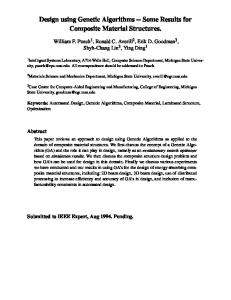
- 22 An interesting question at this point is whether the improved performance of adaptive GABIL is the result of any significant bias adjustment during a run. This is easily monitored and displayed. Figures 4 and 5 illustrate the frequency with which the dropping condition (DC) and adding alternative (AA) operators are used by adaptive GABIL for two target concepts: 3D3C and 4D1C. Since the control bits for each operator are randomly initialized, roughly half of the initial population contain positive control bits resulting in both operators starting out at a rate of approximately 0.5. As the search progresses towards a consistent and complete hypothesis, however, these frequencies are adaptively modified. For both target concepts, the DC operator is found to be the most useful, and consequently is fired with a higher frequency. This is consistent with Table 5, which indicates that GABIL+D outperforms GABIL+A. Furthermore, note the difference in predictive accuracy between GABIL and GABIL+D on the two target concepts. The difference is greater for the 4D1C target concept, indicating the greater importance of the DC operator. This is reflected in Figures 4 and 5, in which the DC operator evolves to a higher firing frequency on the 4D1C concept, in comparison with the 3D3C concept. Similar comparisons can be made with the AA operator. -----------------------------------------------------------------------Insert Figures 4 and 5 about here -----------------------------------------------------------------------Considering that GABIL is now clearly performing the additional task of selecting appropriate biases, these results are very encouraging. We are in the process of extending and refining GABIL as a result of the experiments described here. We are also extending our experimental analysis to include other systems which attempt to dynamically adjust their bias.

6. Related Work on Bias Adjustment Adaptive bias, in our context, is similar to dynamic preference (bias) adjustment for concept learning (see (Gordon, 1990) for related literature). The vast majority of concept learning systems that adjust their bias focus on changing their representational bias. The few notable exceptions that adjust the algorithmic bias include the Competitive Relation Learner and Induce and Select Optimizer combination (CRL/ISO) (Tcheng et. al., 1989), Climbing in the Bias Space (ClimBS) (Provost, 1991), PEAK (Holder, 1990), the Variable Bias Management System (VBMS) (Rendell et. al., 1987), and the Genetic-based Inductive Learner (GIL) (Janikow, 1991). We can classify these systems according to the type of bias that they select. Adaptive GABIL shifts its bias by dynamically selecting generalization operators. The set of biases considered by CRL/ISO includes the strategy for predicting the class of new instances and the method and criteria for hypothesis selection. The set of biases considered by ClimBS includes the beam width of the heuristic search, the percentage of the positive examples a satisfactory rule must cover, the maximum percentage of the negative examples a satisfactory rule may cover, and the rule complexity. PEAK’s

- 23 changeable algorithmic biases are learning algorithms. They are rote learning, empirical learning (with a decision tree), and explanation-based generalization (EBG). GIL is most similar to GABIL, since it also selects between generalization operators. However, it does not use a GA for that selection and only uses a GA for the concept learning task. We can also classify these systems according to whether or not their searches through the space of hypotheses and the space of biases are coupled. GABIL is unique along this dimension because it is the only system that couples these searches. The advantages and disadvantages of a coupled approach were presented in Section 5. We summarize these comparisons in Table 7. -----------------------------------------------------------------------Insert Table 7 about here -----------------------------------------------------------------------The VBMS system is different from the others mentioned above. The primary task of this system is to identify the concept learner (which implements a particular set of algorithmic biases) that is best suited for each problem along a set of problem characteristic dimensions. Problem characteristic dimensions that this system considers are the number of training instances and the number of features per instance. Three concept learners are tested for their suitability along these problem characteristic dimensions. VBMS would be an ideal companion to any of the above-mentioned systems. This system could map out the suitability of biases to problems, and then this knowledge could be passed on to the other systems to use in an initialization procedure for constraining their bias space search.

7. Discussion and Future Work We have presented a method for using genetic algorithms as a key element in designing robust concept learning systems and used this approach to implement a system that compares favorably with other concept learning systems on a variety of target concepts. We have shown that, in addition to providing a minimally biased yet powerful search strategy, the GABIL architecture allows for adding task-specific biases in a very natural way in the form of additional "genetic" operators, resulting in performance improvements on certain classes of concepts. However, the experiments in this paper highlight that no one fixed set of biases is appropriate for all target concepts. In response to these observations, we have shown that this approach can be further extended to produce a concept learner that is capable of dynamically adjusting its own bias in response to the characteristics of the particular problem at hand. Our results indicate that this is a promising approach for building concept learners which do not require a "human in the loop" to adapt and adjust the system to the requirements of a particular class of concepts. The current version of GABIL adaptively selects between two forms of bias taken from a single system (AQ14). In the future, we plan to extend this set of biases to include additional biases from AQ14 and other systems. For example, we would like to implement in GABIL an information theoretic bias, which we believe is primarily responsible for C4.5’s successes.

- 24 The results presented here have all involved single-class learning problems. An important next step is to extend this method to multi-class problems. We have also been focusing on adjusting the lower level biases of learning systems. We believe that these same techniques can also be applied to the selection of higher level mechanisms such as induction and analogy. Our final goal is to produce a robust learner that dynamically adapts to changing concepts and noisy learning conditions, both of which are frequently encountered in realistic environments.

Acknowledgements We would like to thank the Machine Learning Group at NRL for their useful comments about GABIL, J. R. Quinlan for C4.5, and Zianping Zhang and Ryszard Michalski for AQ14.

References Baeck, T., Hoffmeister, F., & Schwefel, H. (1991). A survey of evolution strategies. Proceedings of the Fourth International Conference on Genetic Algorithms (pp. 2 9). La Jolla, CA: Morgan Kaufmann. 1991. Booker, L. (1989). Triggered rule discovery in classifier systems. Proceedings of the Third International Conference on Genetic Algorithms (pp. 265 - 274). Fairfax, VA: Morgan Kaufmann. Braudaway, W. & Tong, C. (1989). Automated synthesis of constrained generators. Proceedings of the Eleventh International Joint Conference on Artificial Intelligence (pp. 583 - 589). Detroit, MI: Morgan Kaufmann. Davis, L. (1989). Adapting operator probabilities in genetic algorithms. Proceedings of the Third International Conference on Genetic Algorithms (pp. 61 - 69). Fairfax, VA: Morgan Kaufmann. De Jong, K. (1987). Using genetic algorithms to search program spaces. Proceedings of the Second International Conference on Genetic Algorithms (pp. 210 - 216). Cambridge, MA: Lawrence Erlbaum. De Jong, K. & Spears, W. (1989). Using genetic algorithms to solve NP-complete problems. Proceedings of the Third International Conference on Genetic Algorithms (pp. 124 - 132). Fairfax, VA: Morgan Kaufmann. De Jong, K. & Spears, W. (1991). Learning concept classification rules using genetic algorithms. Proceedings of the Twelfth International Joint Conference on Artificial Intelligence (pp. 651 - 656). Sydney, Australia: Morgan Kaufmann. Goldberg, D. (1989). Genetic algorithms in search, optimization, and machine learning.

- 25 New York: Addison-Wesley. Gordon, D. (1990). Active bias adjustment for incremental, supervised concept learning. Doctoral dissertation, Computer Science Department, University of Maryland, College Park, MD. Greene, D. & Smith, S. (1987). A genetic system for learning models of consumer choice. Proceedings of the Second International Conference on Genetic Algorithms (pp. 217 - 223). Cambridge, MA: Lawrence Erlbaum. Grefenstette, John J. (1986). Optimization of control parameters for genetic algorithms. IEEE Transactions on Systems, Man, and Cybernetics, Vol. SMC-16, No. 1. Grefenstette, John J. (1989). A system for learning control strategies with genetic algorithms. Proceedings of the Third International Conference on Genetic Algorithms (pp. 183 - 190). Fairfax, Virginia: Morgan Kaufmann. Holder, L. (1990). The general utility problem in machine learning. Proceedings of the Seventh International Conference on Machine Learning (pp. 402 - 410). Austin, Texas: Morgan Kaufmann. Holland, J. (1975). Adaptation in natural and artificial systems. Ann Arbor, MI: The University of Michigan Press. Holland, J. (1986). Escaping brittleness: The possibilities of general-purpose learning algorithms applied to parallel rule-based systems. In R. Michalski, J. Carbonell, T. Mitchell (Eds.), Machine Learning: An Artificial Intelligence Approach. Los Altos: Morgan Kaufmann. Iba, G. (1979). Learning disjunctive concepts from examples. Massachusetts Institute of Technology A.I. Memo 548, Cambridge, MA. Janikow, C. (1991). Inductive learning of decision rules from attribute-based examples: A knowledge-intensive genetic algorithm approach. TR91-030, The University of North Carolina at Chapel Hill, Dept. of Computer Science, Chapel Hill, NC. Koza, J. R. (1991). Concept formation and decision tree induction using the genetic programming paradigm. In H. P. Schwefel and R. Maenner (Eds.), Parallel Problem Solving from Nature. Berlin: Springer-Verlag. Michalski, R. (1983). A theory and methodology of inductive learning. In R. Michalski, J. Carbonell, T. Mitchell (Eds.), Machine Learning: An Artificial Intelligence Approach. Palo Alto: Tioga. Michalski, R. (1986). Learning flexible concepts: Fundamental ideas and a method based on two-tiered representation. In Y. Kodratoff, R. Michalski (Eds.), Machine Learning: An Artificial Intelligence Approach. San Mateo: Morgan Kaufmann.

- 26 Michalski, R., Mozetic, I., Hong, J., & Lavrac, N. (1986). The AQ15 inductive learning system: An overview and experiments. University of Illinois Technical Report Number UIUCDCS-R-86-1260, Urbana-Champaign, ILL. Mozetic, I. (1985). NEWGEM: Program for learning from examples, program documentation and user’s guide. University of Illinois Report Number UIUCDCS-F-85-949, Urbana-Champaign, ILL. Provost, F. (1991). Navigation of an extended bias space for inductive learning, Ph.D. thesis proposal, University of Pittsburgh, Pittsburgh, PA. Quinlan, J. (1986). Induction of decision trees. Machine Learning, 1(1), 81-106. Quinlan, J. (1989). Documentation and user’s guide for C4.5. (unpublished). Rendell, L. (1985). Genetic plans and the probabilistic learning system: Synthesis and results. Proceedings of the First International Conference on Genetic Algorithms (pp. 60 - 73). Pittsburgh, PA: Lawrence Erlbaum. Rendell, L., Seshu, R., & Tcheng, D. (1987). More robust concept learning using dynamically-variable bias. Proceedings of the Fourth International Workshop on Machine Learning (pp. 66 - 78). Irvine, CA: Morgan Kaufmann. Schaffer, J. David & Morishima, A. (1987). An adaptive crossover distribution mechanism for genetic algorithms. Proceedings of the Second International Conference on Genetic Algorithms (pp. 36 - 40). Cambridge, MA: Lawrence Erlbaum. Smith, S. (1983). Flexible learning of problem solving heuristics through adaptive search. Proceedings of the Eighth International Joint Conference on Artificial Intelligence (pp. 422 - 425). Karlsruche, Germany: William Kaufmann. Tcheng, D., Lambert, B., Lu, S., & Rendell, R. (1989). Building robust learning systems by combining induction and optimization. Proceedings of the Eleventh International Joint Conference on Artificial Intelligence (pp. 806 - 812). Detroit, MI: Morgan Kaufmann. Wilson, S. (1987). Quasi-Darwinian learning in a classifier system. Proceedings of the Fourth International Workshop on Machine Learning (pp. 59 - 65). Irvine, CA: Morgan Kaufmann. Utgoff, P. (1988). ID5R: An incremental ID3. Proceedings of the Fifth International Conference on Machine Learning (pp. 107 - 120). Ann Arbor, Michigan: Morgan Kaufmann.

- 27 Appendix 1: Statistical Significance The following three tables give statistical significance results. Table 8 compares adaptive GABIL with all other systems on the nDmC domain (using predictive accuracy). Table 9 makes the same comparison with the convergence criterion. Table 10 compares adaptive GABIL with all other systems on the BC target concept. The column Sig denotes the level of significance of each comparison. The Wins column is "Yes" if adaptive GABIL outperformed the other system; otherwise it is "No". In comparison with all other systems, adaptive GABIL has 19 wins, 7 losses, and 1 tie. At the 90% level of significance, 11 wins and 2 losses are significant. In comparison with the non-GA systems, adaptive GABIL has 10 wins, 4 losses, and 1 tie. Again, at the 90% level of significance, 6 wins and 1 loss are significant. -----------------------------------------------------------------------Insert Table 8 about here ----------------------------------------------------------------------------------------------------------------------------------------------Insert Table 9 about here ----------------------------------------------------------------------------------------------------------------------------------------------Insert Table 10 about here ------------------------------------------------------------------------

- 28 Appendix 2: Artificial Domain Target Concepts This appendix fully describes the target concepts of the artificial domain. There are four features, denoted as F1, F2, F3, and F4. Each feature has four values {v1, v2, v3, v4}. All the target concepts have the following form: 4DmC == d1 v d2 v d3 v d4 3DmC == d1 v d2 v d3 2DmC == d1 v d2 1DmC == d1 For the nD3C target concepts we have: d1 == (F1 = v1) & (F2 = v1) & (F3 = v1) d2 == (F1 = v2) & (F2 = v2) & (F3 = v2) d3 == (F1 = v3) & (F2 = v3) & (F3 = v3) d4 == (F1 = v4) & (F2 = v4) & (F3 = v4) For the nD2C target concepts: d1 == (F1 = v1) & (F2 = v1) d2 == (F1 = v2) & (F2 = v2) d3 == (F1 = v3) & (F2 = v3) d4 == (F1 = v4) & (F2 = v4) Finally, we define the nD1C target concepts: d1 == (F1 = v1) d2 == (F1 = v2) d3 == (F1 = v3) d4 == (F1 = v4)

- 29 -

procedure GA; begin t = 0; initialize population P(t); fitness P(t); until (done) t = t + 1; select P(t) from P(t-1); crossover P(t); mutate P(t); fitness P(t); end. Figure 1. The GA in GABIL.

- 30 -

procedure GA; begin t = 0; initialize population P(t); fitness P(t); until (done) t = t + 1; select P(t) from P(t-1); crossover P(t); mutate P(t); new_op1 P(t); /* additional operators */ new_op2 P(t); ... fitness P(t); end. Figure 2. Extending GABIL’s GA Operators.

- 31 -

procedure GA; begin t = 0; initialize population P(t); fitness P(t); until (done) t = t + 1; select P(t) from P(t-1); crossover P(t); mutate P(t); add_altern P(t); /* +A */ drop_cond P(t); /* +D */ fitness P(t); end. Figure 3. Extended GABIL.

- 32 -

1

1 DC DC

Rate 0.5

Rate 0.5 AA

AA

0 0

200

0 400

0

10

20

30

Generations

Generations

Figure 4: 3D3C.

Figure 5: 4D1C.

- 33 Table 1. Prediction accuracy. __________________________________________________________ Prediction Accuracy __________________________________________________________ TC AQ14 C4.5P C4.5U ID5R IACL GABIL __________________________________________________________ 1D1C 99.8 98.5 99.8 99.8 98.1 95.2 __________________________________________________________ 1D2C 98.4 96.1 99.1 99.0 96.7 95.8 __________________________________________________________ 1D3C 97.4 98.5 99.0 99.1 90.4 95.7 __________________________________________________________ 2D1C 98.6 93.4 98.2 97.9 95.6 92.0 __________________________________________________________ 2D2C 96.8 94.3 98.4 98.2 94.5 92.7 __________________________________________________________ 2D3C 96.7 96.9 97.6 97.9 95.3 94.6 __________________________________________________________ 3D1C 98.0 78.8 92.4 91.2 93.2 90.4 __________________________________________________________ 3D2C 95.5 92.2 97.4 96.7 92.1 90.3 __________________________________________________________ 3D3C 95.3 95.4 96.6 95.6 94.9 92.8 __________________________________________________________ 4D1C 95.8 66.4 77.0 70.2 92.3 89.6 __________________________________________________________ 4D2C 93.8 90.5 95.2 81.3 89.5 87.4 __________________________________________________________ 4D3C 93.5 93.8 95.1 90.3 94.2 88.9 __________________________________________________________ Average 96.6 91.2 95.5 93.1 93.9 92.1 __________________________________________________________ BC 60.5 72.4 65.9 63.4 60.1 68.7 __________________________________________________________

- 34 Table 2. Convergence to 95%. _____________________________________________________ Convergence _____________________________________________________ TC AQ14 C4.5P C4.5U ID5R IACL GABIL _____________________________________________________ 1D1C 13 37 14 12 33 87 _____________________________________________________ 1D2C 28 155 24 26 91 100 _____________________________________________________ 1D3C 57 0 0 0 96 96 _____________________________________________________ 2D1C 28 100 37 44 61 109 _____________________________________________________ 2D2C 43 126 32 40 139 148 _____________________________________________________ 2D3C 86 181 86 75 134 249 _____________________________________________________ 3D1C 34 253 149 137 203 103 _____________________________________________________ 3D2C 78 122 45 52 141 125 _____________________________________________________ 3D3C 195 253 135 123 125 225 _____________________________________________________ 4D1C 82 253 253 255 222 131 _____________________________________________________ 4D2C 78 113 55 255 188 142 _____________________________________________________ 4D3C 154 253 134 224 138 229 _____________________________________________________ Average 73 154 80 104 131 145 _____________________________________________________

- 35 Table 3. Prediction accuracy. _________________________________________ Prediction Accuracy _________________________________________ TC GABIL G+A G+D G+AD _________________________________________ 1D1C 95.2 96.1 97.7 97.7 _________________________________________ 1D2C 95.8 96.2 97.4 97.3 _________________________________________ 1D3C 95.7 95.7 96.7 96.7 _________________________________________ 2D1C 92.0 93.1 97.4 97.0 _________________________________________ 2D2C 92.7 95.0 96.3 96.9 _________________________________________ 2D3C 94.6 94.5 95.8 95.0 _________________________________________ 3D1C 90.4 91.9 96.0 96.6 _________________________________________ 3D2C 90.3 91.6 94.5 94.6 _________________________________________ 3D3C 92.8 92.7 94.2 92.9 _________________________________________ 4D1C 89.6 90.9 95.1 95.2 _________________________________________ 4D2C 87.4 89.7 93.0 92.7 _________________________________________ 4D3C 88.9 89.2 92.3 90.0 _________________________________________ Average 92.1 93.1 95.5 95.2 _________________________________________ BC 68.7 69.1 71.5 72.0 _________________________________________

- 36 Table 4. Convergence to 95%. ______________________________________ Convergence ______________________________________ TC GABIL G+A G+D G+AD ______________________________________ 1D1C 87 58 28 32 ______________________________________ 1D2C 100 85 59 68 ______________________________________ 1D3C 96 97 94 97 ______________________________________ 2D1C 109 90 42 42 ______________________________________ 2D2C 148 93 82 55 ______________________________________ 2D3C 249 250 136 250 ______________________________________ 3D1C 103 104 54 39 ______________________________________ 3D2C 125 127 76 62 ______________________________________ 3D3C 225 240 161 240 ______________________________________ 4D1C 131 120 67 62 ______________________________________ 4D2C 142 133 75 75 ______________________________________ 4D3C 229 253 166 248 ______________________________________ Average 145 138 87 106 ______________________________________

- 37 Table 5. Prediction accuracy. ___________________________________________________ Prediction Accuracy ___________________________________________________ TC GABIL G+A G+D G+AD Adaptive ___________________________________________________ 1D1C 95.2 96.1 97.7 97.7 97.6 ___________________________________________________ 1D2C 95.8 96.2 97.4 97.3 97.4 ___________________________________________________ 1D3C 95.7 95.7 96.7 96.7 96.5 ___________________________________________________ 2D1C 92.0 93.1 97.4 97.0 96.1 ___________________________________________________ 2D2C 92.7 95.0 96.3 96.9 96.2 ___________________________________________________ 2D3C 94.6 94.5 95.8 95.0 95.4 ___________________________________________________ 3D1C 90.4 91.9 96.0 96.6 95.9 ___________________________________________________ 3D2C 90.3 91.6 94.5 94.6 94.0 ___________________________________________________ 3D3C 92.8 92.7 94.2 92.9 94.7 ___________________________________________________ 4D1C 89.6 90.9 95.1 95.2 95.8 ___________________________________________________ 4D2C 87.4 89.7 93.0 92.7 92.8 ___________________________________________________ 4D3C 88.9 89.2 92.3 90.0 92.1 ___________________________________________________ Average 92.1 93.1 95.5 95.2 95.4 ___________________________________________________ BC 68.7 69.1 71.5 72.0 70.3 ___________________________________________________

- 38 Table 6. Convergence to 95%. _______________________________________________ Convergence _______________________________________________ TC GABIL G+A G+D G+AD Adaptive _______________________________________________ 1D1C 87 58 28 32 34 _______________________________________________ 1D2C 100 85 59 68 58 _______________________________________________ 1D3C 96 97 94 97 97 _______________________________________________ 2D1C 109 90 42 42 50 _______________________________________________ 2D2C 148 93 82 55 80 _______________________________________________ 2D3C 249 250 136 250 120 _______________________________________________ 3D1C 103 104 54 39 53 _______________________________________________ 3D2C 125 127 76 62 70 _______________________________________________ 3D3C 225 240 161 240 128 _______________________________________________ 4D1C 131 120 67 62 55 _______________________________________________ 4D2C 142 133 75 75 80 _______________________________________________ 4D3C 229 253 166 248 130 _______________________________________________ Average 145 138 87 106 80 _______________________________________________

- 39 Table 7. Comparison of system characteristics. ___________________________________________________________ System Bias Space Searches GA ___________________________________________________________ CRL/ISO hypothesis selection criteria uncoupled no prediction strategy ___________________________________________________________ ClimBS beam width uncoupled no hypothesis coverage ___________________________________________________________ PEAK learning strategy uncoupled no ___________________________________________________________ VBMS concept learners uncoupled no ___________________________________________________________ GIL generalization operators uncoupled yes ___________________________________________________________ Adaptive GABIL generalization operators coupled yes ___________________________________________________________

- 40 Table 8. Predictive Accuracy on nDmC. _______________________ System Sig Wins _______________________ AQ14 80% No _______________________ C4.5P 80% Yes _______________________ C4.5U < 80% No _______________________ ID5R < 80% Yes _______________________ IACL 80% Yes _______________________ GABIL 95% Yes _______________________ G+A 95% Yes _______________________ G+D < 80% No _______________________ G+AD < 80% Yes _______________________

- 41 Table 9. Convergence on nDmC. _______________________ System Sig Wins _______________________ AQ14 < 80% No _______________________ C4.5P 95% Yes _______________________ C4.5U < 80% Tie _______________________ ID5R < 80% Yes _______________________ IACL 95% Yes _______________________ GABIL 95% Yes _______________________ G+A 95% Yes _______________________ G+D < 80% Yes _______________________ G+AD < 80% Yes _______________________

- 42 Table 10. Predictive Accuracy on BC. _____________________ System Sig Wins _____________________ AQ14 95% Yes _____________________ C4.5P 95% No _____________________ C4.5U 95% Yes _____________________ ID5R 95% Yes _____________________ IACL 95% Yes _____________________ GABIL 90% Yes _____________________ G+A 80% Yes _____________________ G+D 80% No _____________________ G+AD 95% No _____________________