Concepts and Methods in Fault-tolerant Control Tutorial at American Control Conference, June 2001
Mogens Blanke1 , Marcel Staroswiecki2 and N. Eva Wu3 1
Oersted-DTU, Department of Automation, Technical University of Denmark, 2 3
LAIL-CNRS, EUDIL, University of Lille, France
Deptartment of Electrical Engineering, Binghamton University, NY, USA
[email protected],
[email protected],
[email protected]
Abstract Faults in automated processes will often cause undesired reactions and shut-down of a controlled plant, and the consequences could be damage to technical parts of the plant, to personnel or the environment.Faulttolerant control combines diagnosis with control methods to handle faults in an intelligent way. The aim is to prevent that simple faults develop into serious failure and hence increase plant availability and reduce the risk of safety hazards. Fault-tolerant control merges several disciplines into a common framework to achieve these goals. The desired features are obtained through on-line fault diagnosis, automatic condition assessment and calculation of appropriate remedial actions to avoid certain consequences of a fault. The envelope of the possible remedial actions is very wide. Sometimes, simple re-tuning can suffice. In other cases, accommodation of the fault could be achieved by replacing a measurement from a faulty sensor by an estimate. In yet other situations, complex reconfiguration or online controller redesign is required. This paper gives an overview of recent tools to analyze and explore structure and other fundamental properties of an automated system such that any inherent redundancy in the controlled process can be fully utilized to maintain availability, even though faults may occur. 1 .
1 Introduction Automated systems are vulnerable to faults. Defects in sensors, actuators, in the process itself, or within the controller, can be amplified by the closed-loop control systems, and faults can develop into malfunction of the loop. The closed-loop control action may hide a fault from being observed. A situation is reached in which a fault eventually develops into a state where loop-failure is inevitable. A control-loop failure will easily cause 1 The authors wish to acknowledge support from the following organizations: M. Blanke and M. Staroswiecki obtained support by the European Science Foundation under the COSY network grant, N. E. Wu obtained support by the NSF (Grant ECS-9615956), the Xerox Corporation (Grant HE 1321-98), and NASA (Cooperative Agreement NCC-1-336)
production to stop or system malfunction at a plant level. With economic demand for high plant availability, and an increasing awareness about the risks associated with system malfunction, dependability is becoming an essential concern in industrial automation. A costeffective way to obtain increased dependability in automated systems is to introduce fault-tolerant control (FTC). This is an emerging area in automatic control where several disciplines and system-theoretic issues are combined to obtain a unique functionality. A key issue is that local faults are prevented from developing into failures that can stop production or cause safety hazards. Automation for safety-critical applications, where no failure could be tolerated, requires redundant hardware to facilitate fault recovery. Fail-operational systems are made insensitive to any single point component failure. Fail-safe systems make controlled shut-down to a safe state when a sensor measurement indicates a critical fault. In contrast, fault-tolerant control systems, employ redundancy in the plant and its automation system to make ”intelligent” software that monitors behavior of components and function blocks. Faults are isolated, and appropriate remedial actions taken to prevent that faults develop into critical failures. The overall FTC strategy is to keep plant availability and accept reduced performance when critical faults occur. One way of achieving fault-tolerance is to employ fault diagnosis schemes on-line. A discrete event signal to a supervisor-agent is generated when a fault is detected. This, in turn activates accommodation actions [4], which can be pre-determined for each type of critical fault or obtained from real-time analysis and optimization. Systematic analysis of fault propagation [1], [6] was shown to be an essential tool for determination of severity of fault effects and for assessment of remedial actions early in the design phase. A semantics for services based on generic component models was developed in [35], [15] and a graphic analysis was found to be very
useful. The properties of combined fault diagnosis and control were treated in [29]. [36] focus on the use of fault estimation within a reliable control framework, using the definitions given by [39]. The methods for re-configuration design are comparatively new within the FTC domain. A few schemes have come into real application. Predetermined design for accommodation was demonstrated for a satellite in [7], and [6]. Techniques using logic inference on qualitative models were used in [26] and [27]. A related area is the control of discrete-event dynamic systems (DEDS) which have a known structure with pre-determined events that occur with unknown instants and sequence [41]. Diagnosis for DEDS was treated in [30] and [25]. DEDS is a sub-class of FTC, where events are not pre-determined and system structure can change when faults occur. Concerning implementation, a correct and consistent control system analysis should always be followed by equally correct software implementation. This is particularly relevant for the supervisory parts of an FTC scheme [20]. Testing of the FTC elements is difficult since it is difficult to replicate the real conditions under which faults occur. Well planned software architecture and implementation are thus crucial issues for FTC implementation. A study of the use of object-oriented programming architectures was described by [24]. The FTC area is hence very wide and involves several areas of system theory. One overview [29] emphasized many algorithmic essentials and the role of FDI. Another [4] presented an engineering view of the means to obtain FTC. Formal definitions were introduced in [3]. Analysis of structure was covered in [15], [31], [20]. Measures of recoverability were discussed in [14], [15] and [44]. Quantitative techniques to assess the reliability of FTC implementations was the subject of [43], [42]. This tutorial paper focus on the methodological issues in analysis for FTC. The severity of faults is first addressed through analysis of fault propagation, which provides a list of faults that should be stopped from developing into failure due to the severity of their end effects. The possibilities to detect and stop propagation of particular faults are then dealt with. A structural analysis technique is introduced, which uses graph theory to determine which redundancy exists in the system and thus shows the possibilities to diagnose and handle particular faults. The reliability of fault-tolerant systems is furthermore treated. Next, implementation of a fault-tolerant control scheme is proposed as a layered structure where an autonomous supervisor implements detection and reconfiguration using the necessary logic. The overall development strategy is finally summarized and an example illustrates features of the methods.
2 Basic Definitions As this is a new engineering field, it is particularly important to define the terminology carefully. A short list is enclosed with the main terms. A longer list can be found in the IFAC - SAFEPROCESS terminology definition [19]. In addition to terminology, different control methods should be clearly distinguished. Definitions are included to specify explicitly what should be understood by the term fault-tolerant control. 2.1 Terminology • Constraint: a functional relation between variables and parameters of a system. Constraints may be specified in different forms, including linear and nonlinear differential equations, and tabular relations with logic conditions between variables. • Coverage: the conditional probability that the failure of a subsystem that would have otherwise caused the system failure has been detected, identified, and predicted to be recoverable through accommodation or reconfiguration, given that the subsystem failure has occurred. • Controlled system: a physical plant under consideration with sensors and actuators used for control • Fail-operational : a system, which is able to operate with no change in objectives or performance despite of any single failure. • Fail-safe: a system, which fails to a state that is considered safe in the particular context. • Fault-tolerance: the ability of a controlled system to maintain control objectives, despite the occurrence of a fault. A degradation of control performance may be accepted. Fault-tolerance can be obtained through fault accommodation or through system and /or controller reconfiguration. • Fault-accommodation: change in controller parameters or structure to avoid the consequences of a fault. The input-output between controller and plant is unchanged. The original control objective is achieved although performance may degrade. • Reconfiguration: change in input-output between the controller and plant through change of controller structure and parameters. The original control objective is achieved although performance may degrade. • Supervision: the ability to monitor whether control objectives are met. If not, obtain/calculate a
revised control objective and a new control structure and parameters that make a faulty closed loop system meet the new modified objective. Supervision should take effect if faults occur and it is not possible to meet the original control objective within the fault-tolerant scheme. • Structure graph: A bi-partite graph representing the general dynamic equations (constraints) that describe the system. Constraints that are isomorphic mappings are denoted by double arrows on arcs. Non-isomorphic mappings are indicated by unidirectional arcs in the graph. 2.2 The control problem A standard control problem is defined by a control objective O, a class of control laws U, and a set of constraints C. Constraints are functional relations that describe the behavior of a dynamic system. Linear or nonlinear differential equations constitute very useful representations of constraints for many physical systems. Other types of models are necessary in other cases. The constraints define a structure S and parameters θ of the system. Solving the control problem means to find in U a control law U that satisfies C while achieving O . Some performance indicator J could be associated with a control objective O. When several solutions exist, the best one is selected according to J. The control problem is defined as: Definition 1 The control problem: Solve the problem < O, S, θ, U > . Now suppose that we only know the set to which the actual value belongs, e.g. due to time-varying parameters or uncertainty, the control problem is now to achieve O under constraints whose structure is S and whose parameters belong to a set Θ. Two solution approaches can be defined: robust control minimizes the discrepancy over Θ of the achieved results, while adaptive conˆ trol first estimates the ”true” parameter θ. Definition 2 The robust control problem : Solve < O, S, Θ, U > where Θ stands for a set of possible θ values. The robust control problem is illustrated in Figure 1. Definition 3 The adaptive control problem : Solve < ˆ U > where θˆ ∈ Θ is estimated as part of the O, S, θ, adaptation. The next problem extension is < O, S, Θ, U > where S stand for a given set of constraint structures. Define some deterministic automaton Γ, which shifts from
Robust control Plant sp Control Design
qc: qp
x& c = fc (x c , qc , y) u = hc (x c , qc , y)
y
u
x& p = fp (x p , q p , u )
Gp xp
y = hp (x p , q p , u )
Figure 1: Robust control illustrated in the hybrid system framework. Robust control deals with the estimated uncertainty of the plant parameters θ
one pair (S, θ) ∈ S × Θ to another one (hybrid control). The problem is to achieve O under a sequence of constraints which is defined by Γ. When O itself is decomposed into a sequence of goals, the problem becomes < O, S, Θ, U > with Γ shifting from one quadruple (O, S, θ, U ) ∈ O × S × Θ × U to another. Next, consider < O, S, Θ, U > with uncertain knowledge about (S, θ). O has to be achieved under constraints whose structure and parameters are partly or fully unknown, except that (S, θ) belongs to S ×Θ. Let a control objective O and a nominal system (S ∗ , θ∗ ) be ˆ ˆ θ) given. Let (S, θ) be the actual constraints and (S, the estimated ones. Nominal control obviously solves < O, S ∗ , θ∗ , U >. When a fault occurs, (S, θ) 6= (S ∗ , θ∗ ) and nominal control is no longer suitable. This is a generalization of the robust and adaptive control problems. Both the parameters and the structure of constraints may change when faults occur. Definition 4 The fault-tolerant ³ ´control problem: ˆ Θ, ˆ U > where S, ˆΘ ˆ is the set of posSolve < O, S, sible structures and parameters of the³ faulty ´ system. ˆΘ ˆ could be Where diagnosis is available, the set S, provided by a diagnosis task. The architecture of a fault-tolerant control system is illustrated in Figure 2. A fault is a discrete event that acts on a system and by that changes some of the properties of the system. The goal of fault-tolerant control is in turn to respond to the occurrence of a fault such that the faulty system still is well behaved. Due to these discrete nature of fault occurrence and reconfiguration, FTC systems are hybrid in nature ([14],[13]). In the Figure, σf denotes fault events, σa are control events reconfiguring the system and qc the control mode, which selects a control law. The actual physical mode qp of the plant my be viewed as the discrete state of an automaton which is driven by plant inter-
nal events σp , the fault events σf and the control events σa . Many different approaches can be used to solve the ˆ Θ, ˆ U > [29]. However, robust FTC problem < O, S, approaches, which achieve the goal for any pair (S, θ) are clearly unrealistic in the general case.
Diagnosis
Supervisor automaton
Gd sf - fault
sa
sc
Plant sp
Control
qc x&c = fc (xc , qc , u) y = hc (xc , qc , u)
qp y
u
Gp
x& p = fp (x p , qp , u)
xp
y = hp (x p , qp , u)
y
Figure 2: The plant can change in a discrete way through change in states, a plant fault can cause a discrete event. Plant architecture can be changed by switch-over functions. Parameters or structure of the controller can be changed by logic in a supervisor automaton. The automaton gets its input from fault diagnosis.
We define two subsets of fault-tolerant control, one is accommodation, the other reconfiguration. Definition 5 Fault accommodation : Solve the control ˆ U > where (S, ˆ is the estimate of ˆ θ, ˆ θ) problem < O, S, the actual constraints, e.g. provided by fault diagnosis algorithms. The fault(s) can thus be accommodated if < ˆ U > has a solution. If accommodation is not ˆ θ, O, S, possible, another problem has to be stated, by finding a pair (Σ, τ ) among all feasible pairs S × Θ, such that < O, Σ, τ, U > has a solution. A pair (Σ, τ ) is considered feasible if it belongs to the fault-free parts of the ³ faulty ´ system. Fault diagnosis may identify a ˆ ˆ set S, Θ to give an estimate of the constraints of the faulty system. This is not a necessary prerequisite but the availability of such estimate will improve the possibility of finding said solution. This procedure is an active approach, the control is changed as a consequence of our knowledge of the new control problem. Reconfiguration is hence defined as follows, a new set of sysDefinition 6 Reconfiguration : Find ¯ ¯ ˆ ˆ tem constraints (Σ, τ ) ∈ (S, Θ) ¯(S, Θ) such that the control problem < O, Σ, τ, U > has a solution. Activate
this solution. The choice of a new set of constraints will imply that input-output relations between controller and plant are changed. The difference between accommodation and reconfiguration whether input-output (I/O) between controller and plant is changed. Reconfiguration implies use of different I/O relations between the controller and the system. Switch of the system to a different internal structure, to change its mode of operation, is an example of such I/O switching. Accommodation does not use such means. Both fault accommodation and system reconfiguration strategies may need new control laws in response to faults. They also have to manage transient behavior, which result from the change of control law or change of the constraints’ structure. It is noted that the set of feasible pairs S × Θ may depend on the fault(s). If such a pair does not exist, this means that O can be achieved neither by fault accommodation nor by system reconfiguration. The only possibility is thus to change the objective O. The most general problem is defined by the triple < O, S, Θ, U > where O is a set of possible control objectives. In view of its practical interpretation, < O, S, Θ, U > is defined as a supervision problem in which the system goal is not pre-defined, but has to be determined at each time taking into account the actual system possibilities. A supervision problem is thus an FTC problem associated with a decision problem: when faults are such that fault-tolerance cannot be achieved, the system goal itself has to be changed [33]. When far-reaching decisions with respect to the system goal have to be taken, human operators are generally involved. Definition 7 Supervision: Monitor the triple (O, S, θ) to determine whether the control objective is achieved. If this is not the case, and the fault tolerant problem does not have a solution, then find a relaxed objective Γ ∈ O and a pair (Σ, τ ) ∈ S×Θ, such that the relaxed control problem < Γ, Σ, τ, U > has a solution. If no such triple exists, failure is unavoidable. This can be a design error or a deliberate choice to accept certain failure scenarios, e.g. for reasons of cost/benefit or small likelihood for a certain event. The choice of a new objective can be made autonomously in rare cases only. Most commonly, human intervention is needed, using decision support from the diagnosis and overall goals for the plant [23], [34]. It should be noted that the choice of Γ could be made to include the fail-to-safe
condition where control is no longer active but plant safety is not at stake. Definition 8 A system is recoverable from a fault iff a solution exists to at least one of the problems < ˆ U > and < O, Σ, τ, U > . ˆ θ, O, S, Definition 9 A system is weakly recoverable if a solution exists to < Γ, Σ, τ, U >.
Definition 10 Fault propagation matrix: boolean mapping of component faults fc ∈ F onto effects ec ∈ E, M : F × E y {0, 1} ; ½ 1 if fcj = 1 =⇒ eci = 1 mij = 0 otherwise An FMEA scheme can be expressed as eci ← Mfi ⊗ fci
3 Analysis of Fault Propagation The first step in a fault-tolerant design is to determine which failure modes could severely affect the safety or availability of a plant. Analysis of failure of parts of a system is a classical discipline and the failure mode and effects analysis (FMEA) is widely used and appreciated in industry. The traditional FMEA does not support analysis of the handling of faults, only of their propagation. In automated systems, when the goal of fault-tolerance is to continue operation, if this is at all possible. An extended method for fault propagation analysis (FPA) was hence suggested in [1] using an algebraic approach for propagation analysis. The aim is to show end effects of faults, and assist in designing for fault tolerance such that end effects with severe consequences are stopped if the system structure makes this possible. If the FPA analysis finds that serious failure can occur due to certain faults, these are included in a list of fault effects to be detected. Whether this is possible is disclosed in a later analysis of structure that shows which redundant information is available in the system [35], [9], [10]. The final step will then be to find actions, preferably within the software of the controller, that can accommodate the fault and prevent the serious end effects from occurring. Analysis of the quality measures of recovery were treated in [14], [31], 3.1 Fault propagation For the reasons given above, fault analysis needs to incorporate analysis throughout a system. In order to do this a component-based method was introduced [1], in which possible component faults are identified at an early stage of design. The method uses the FMEA description [22], [17] of components as a starting point. In this context components are sensors, valves, motors, programmable functions etc.. Programmable parts are considered as consisting of separate function blocks that can be treated similarly to physical components in the analysis, bearing in mind that their properties may be changed by software modifications if so desired. An FMEA scheme shows how fault effects out of the component relate to faults at inputs, outputs, or parts within the components.
(1)
where Mfi is a Boolean matrix representing the propagation. The operator ⊗ is the inner product disjunction operator that performs the boolean operation ecik ← (mik1 ∧ fci1 ) ∨ (mik2 ∧ fci2 ) ... ∨ (mikn ∧ fcin ) (2) When effects propagate from other components, we get, at level i: · ¸ fci eci ← Mfi ⊗ (3) ec(i−1) This is a surjective mapping from faults to effects: there is a unique path from fault to end effect, but several different faults may cause the same end effect. System descriptions are obtained from interconnection of component descriptions. Merging three levels gives the end effects at the third level, I µ fc3 ·0 ¸¶ ⊗ fc2 (4) I 0 ec3 ← 0 Af2 ⊗ fc1 0 Af1 Eventually, end effects at the system level are reached. A mapping of observed effects to possible faults are ob¡ ¢−1 ¡ ¢−1 tained through fc = Mf ec . And Mf = MT f since M is Boolean. Analysis of the system matrix can easily show where in the system the propagation should be detected and stopped. When there is no logical feedback involved, the result is the capability of isolation of fault effects at any level. If feedback is involved, we have a principal difficulty: if a cut in the graph of a boolean loop is stable - the two sides of the cut remain equal after one propagation around the loop - then the loop is a tautology and can be eliminated. If not, no boolean solution exists. A ”dedicated loop treatment” was employed in [2] to define the two sides of a loop cut as additional input and output, and leave the further judgement to the designer. This shortcoming is shared by several methods in reliability engineering. The principal difficulty is caused by the binary modelling of faults and their propagation.
With this obstacle in mind, fault propagation analysis should be the first step in a fault-tolerant design. The systematic approach forced upon the designer should not be underestimated, and might even be an asset as an essential part of the safety assessment needed in many industrial designs. Experience from applying fault propagation analysis to larger systems show that we might need to include occurrence of one fault and the non-occurrence of another in the description [6]. This means extending fi £ ¤T to fi , ¯ fi in the above expressions.
4 Analysis of Structure The structural model of a system, see [32] and [11], is a bi-partite graph that represents the relations between system variables and parameters (known and unknown), and the dynamic equations (constraints) that describe the system behavior. Analysis of the systemstructure graph will reveal any system redundancy, and particular sub-systems can be identified which can be exploited to obtain fault-tolerance. 4.1 Structural model Let F = {f1 , f2 , ..fm } be the set of the constraints which represent the system model and Z = {z1 , z2 , ..zn } the set of the variables and parameters. With K the subset of the known and X the subset of the unknown elements in Z, Z = K ∪ X. Z is allowed to contain time derivatives, so that dynamic systems as well as static ones can be described by their structure. Definition 11 The structure graph of a system is a bipartite graph (F, Z, A) where elements in the set of arcs A ⊂ F × Z are defined by : (fi , zj ) ∈ A iff the constraint fi applies to the variable or parameter zj , ( fi ∈ F with i = 1, ...m and zj ∈ Z with j = 1, ...n). The structure-graph is hence a bi-partite. A graph is bipartite (see [16]) if its vertices can be separated into two disjoint sets F and Z in such a way that every edge has one endpoint in F and the other in Z. Definition 12 A sub-system is a pair (φ, Q(φ)), where φ ∈ P(F ) is a subset of F, and Q is defined by Q:
P(F ) → P(Z); φ → Q(φ) = {zj |
∃fi ∈ φ such that (fi , zj ) ∈ A}
In this definition, a sub-system is any subset of the system constraints φ along with the related variables Q( φ) ∈ Z. There are no specific requirements to the choice of the elements in φ. P(F ) is the set of the
subsets of F and it contains all possible sub-systems. The sub-graph that is related to a sub-system is the structure of the sub-system, (φ, Q(φ)). Sub-systems are used to find alternate paths through a structure-graph. When a fault has occurred we need to exploit alternative ways to access variable(s) xf ∈ X affected by the fault. The design task is to express xf through alternative subsystem(s) and eventually through associated known variable(s), in K. This means to exploit analytic redundancy relations in the system. 4.2 Matching on a structure-graph and canonical decomposition The set of constraints is separated in FK , those that apply only to known variables, and FX , which apply to unknown elements in Z, F = FK ∪ FX . We are interested in the analysis of the sub-graph G(FX , X, AX ) in order to determine which analytic redundancy relations exist that can help access a particular unknown variable. If redundant sub-graphs are available, then the particular variable could be observed or controlled via the redundant path should a fault occur in the other.
Definition 13 Let a ∈ AX , F (a) ∈ FX and X(a) ∈ X, such that a = (F (a), X(a)). A matching M is a subset of AX such that : ∀a and b ∈ M, F (a) 6= F (b) and X(a) 6= X(b). A complete matching on FX : ∀f ∈ FX ∃x ∈ X such that (f, x) ∈ M A complete matching on X: ∀x ∈ X ∃f ∈ FX such that (f, x) ∈ M .
4.3 Interpretation From the matching definition, each pair a = (F (a), X(a)) can be interpreted as follows : X(a) is a consequence of the constraint F (a) in which all the variables Q(F (a)) except X(a) would have values imposed from the rest of the system and the environment. However, not all matching can receive this nice interpretation, and the set of the possible causality assignments (causal matching) is only a sub-set of the possible matching. Using causal matching, the analytic redundancy relations appear on the structural graph as alternated chains, making it easy to design the parity relations used for fault diagnosis. Moreover, a causal graph can be associated with each causal matching on a structural graph, providing structural tools for alarm filtering and reconfigurability analysis [31]. The structural approach can thus treat the all issues of principal interest regarding redundancy for sensing and actuation possibilities in a plant.
5 Example: Propulsion Control To illustrate the methods of analysis, we consider a propulsion system , which was defined as a COSY benchmark on fault detection and fault-tolerant control [21], [20]. This example is taken from the marine area but applies in principle to aeroplane propulsion as well. 5.1 Constraints Developed thrust and torque are functions of pitch u2 , shaft speed x1 and ship speed x2 .
f4
y1
f1
x1
y2
f2
x2
u2
f8
Qprop f7 f12
Qeng
f6
.
x1
f9c Tprop
f10
f14
It,nom
Ky
f5
Ky,nom
u1
f3
u1 m
R(x2)
f15
Rnom
.x
2
f13
f11
Figure 3: The system-structure graph for vessel propul-
Measurements are f1 f2 f3 f4
: : : :
y1 = x1 y2 = x2 u1m = u1 u2m = u2
sion example. Constraints are functional relations between parameters and variables
(5) 5.2 Analysis of Structure We first observe which variables belong to the sets F (15 elements), X(12 elements) and K(7 elements):
Engine and dynamic shaft equation f5 : Ky = Ky,nom f6 : Qeng = Ky u1 f7 : It x˙ 1 = −Qprop + Qeng
(6)
f8 : Qprop = Qn|n||ϑ| |u2 | |x1 | x1 + Q|n|uϑ u2 |x1 | x2 f9 : Tprop = T|n|nϑ u2 |x1 | x1 + Tnu x1 x2 (7) Vessel speed and resistance, mx˙ 2 = −R(x2 ) + (1 − t)Tprop R(x2 ) = X|u|u |x2 | x2
(8)
The differentials x˙ 1 and x˙ 2 are the integrals of x1 and x2 , respectively. Since integration of the derivative can not determine the related state variable, due to unknown initial value, the arrows in the structure diagram are unidirectional. f12 : f13 :
x˙ 1 = x˙ 2 =
d dt x1 d dt x2
(9)
This illustrates the difference between observability and calculability, as defined in structure analysis. Finally, parameters are assumed known. All such parameters should have identity constraints associated with them. For brevity, only two are shown in the Figure, f14 : f15 :
It = It,nom R(·) = R (·)nom
F = {f1 , f2 ...f15 } K = {y1 , y2 , um1 , um2 , Ky,nom , It,nom , Rnom }
Propeller
f10 : f11 :
u2m
It
(10)
The control objective is to obtain desired cruising speed while meeting constraints on the shaft’s angular speed. The system’s structure graph is shown in Figure 3 The ship benchmark deals with several faults. One of those is a sensor fault in shaft speed measurement. This means constraint f1 is violated. This example investigates which redundancy relations exist to reconstruct this measurement.
(11) (12)
X = {x1 , x˙ 1 , x2 , x˙ 2 , u1 , u2 , Qeng , Qprop , Tprop , Ky , It , R(·)} (13) It is noted that FK = ∅ as there is no direct redundancy in this system. A structural analysis of the system gives that the set A of Definition 11 could be ordered as one matrix of dimension (dim(F ), (dim(X) + dim(K))). Alternatively, individual entries are listed, and sparse matrix techniques could be used in the analysis, A = {(f 1 , y 1 ), (f 1 , x1 ), (f 2 , y 2 ), (f 2 , x2 ), (f3 , u1m ), (f3 , u1 ), (f 4 , u2m ), (f 4 , u2 ), (f 5 , K y ), (f 5 , K y,nom ), (f 6 , Qeng ), (f 6 , K y ), (f 6 , u1 ), (f 7 , Qprop ), (f 7 , Qeng ), (f7 , I t ), (f7 , n1 ), (f 8 , u2 ), (f 8 , x1 ), (f 8 , x2 ), (f 8 , Qprop ), (f 9 , x2 ), (f 9 , u2 ), (f 9 , x1 ), (f 9 , T prop ), (f 10 , x˙ 2 ), (f 10 , R(x2 )), (f 10 , T prop ), (f 11 , R), (f 11 , x2 ), (f 12 , x˙ 1 ), (f12 , x1 ), (f 13 , x˙ 2 ), (f13 , x2 ), (f14 , I t ), (f14 , I t,nom ), (f 15 , R), (f 15 , Rnom ),}
(14)
The set of sub-systems comprise sets of selected constraints, with associated variables, and the combinations of such sets, ϕ = {(f1 , y1 , x1 ) , ..., (f11, R(x2 ) , x2 , Rnom ), ..} ∪ {(f1 , f2 , y1 , x1 , y2 , x2 ), ...} ∪ {(fi , fj , yk , ...), ...} ...
(15)
X x1 x˙ 1 x2 x˙ 2 u1 u2 Qeng Qprop Tprop Ky It R(·)
M. 1 1 7 2 10 3 4 6 8 9 5 14 15
M. 2 8 12 13 10 3 4 6 7 9 5 14 15
M. 3 12 7 2 13 3 4 6 8 10 5 14 11
M. 4 9 12 2 13 3 4 6 7 10 5 14 11
Table 1: Four examples on complete matching on X for the example
at the bottom level for controls and at the autonomous supervisor level for diagnosis, Figure 2. This section attempts to establish such a linkage in a quantitative manner. Computer / effector
λ1 Computer / effector
λ1
Computer / effector
λ1 Computer / effector
Several complete matchings on X exist, and some of these are listed in table 1. In the table, the elements refer to the constraints (as elements in A) that are associated with each variable in X. In match 1, x1 is associated with f1 whereas it is associated with f8 in matching number 2. In the non-faulty case, x1 is assessed through measurement, formally through constraint 1 and the arc (f1 , x1 , (f1 , y1 )). If the fault in f1 occurs, analytic redundancy relations should be found that reconstruct x1 from other relations. This is possible from matchings 2, 3 or 4, which do not include f1 . In constructing the analytic redundancy relations, one has to consider the causality, it is not possible to calculate x1 from x˙ 1 through f12 as listed in matching 3, since the initial value at the start of calculation is unknown. Observer techniques could, nevertheless, be employed to provide a useful - and asymptotically correct - estimate, if observation was started well in advance of the fault incident. The conclusion is that in the faulty case, we could use two remaining ARR’s, one uses constraint f8 , the other f9 .
6 Reliability issues in FTC Systems Reliability has always been a subjective concern in the analysis and design of fault-tolerant control systems. However, it is rarely associated with an objective criterion that guides a design. This predicament is due to the fact that standard reliability assessment techniques are not geared toward systems with the type of redundancy that is involved in fault tolerant control systems. Therefore, it is difficult to establish a functional linkage between the reliability at the plant wide control level, and the performance defined in the conventional sense
λ1
Actuator
λ2 Actuator
λ2 Actuator
λ2 Actuator
λ2
Surface 1a
λ3 Surface 1b
λ3
Lateral state(s)
Surface 2a
λ3 Surface 2b
λ3
Figure 4: Functional dependence of the lateral direction control block. Experimental aircraft example
6.1 Reliability assessment To understand some of the issues peculiar to fault tolerant control systems, we start with a simple reliability model of a fault tolerant control system. Figure 4 shows the functional dependencies of subsystems in the lateral-directional control effector block (associated with control surfaces and actuators) within a fault tolerant flight control system (FTFCS). The diagram reflects the available redundant control authorities in the system and the extent such redundancy is utilized for failure recovery. The subsystems involved in this block are computer/effector (C/E) interface subsystems, actuator subsystems, and control surfaces. This particular configuration is similar to that in an AFTI-16 aircraft where surface types #1 and #2 represent stabilators and flaps [42], respectively. Each actuator is preceded by a group of three or four active identical C/E subsystems, and followed by a control surface. This control effector block is the focus of our study because it involves the management of functionally redundant control effectors at the plant wide control level. Other preceding blocks not showing in the figure include a computer power supply block, an I/O control module block, a pilot command sensor block and an aircraft state sensor block. Each of these blocks is of quadruplex architecture (group of four active identical subsystems). The block following the lateral-directional block is a pitch control effector block where a rudder and two canards are involved. The functional dependency of the FTFCS altogether is described by a parallel-toseries interconnection scheme. For the effector block of Figure 4 to be operational, we require that three out of four channels be operational. This means that the three remaining channels must work in concert to ac-
commodate the failure in one. Safety requirement considered for all quadruplex computer/effector interface subsystems is Fail-Operational/Fail-Operational/FailOperational/Loss-of-Control.
In obtaining a reliability model and determining reliability requirements, detailed analysis and deep understanding of the system are necessary. In addition, unlike in a digital system where redundancy can be described by 0’s (nonexistent) or 1’s (existent), the level of redundancy often needs to be quantified and measured properly in fault tolerant control systems. The calculation of attainable moments affordable by effectors [5] for control of aircraft movement in all axes is an example of the effort along this direction. The architecture shown in Figure 2 must be understood as an effective redundancy configuration. In reality, accommodation/reconfiguration schemes in fault tolerant control systems can be much more complicated than the traditional redundancy management scheme, such as a majority voting. Therefore, several risk factors are involved in making a decision in a accommodation/reconfiguration action, – overly slow or severe transients – false alarm – miss detection – false identification – false accommodation/reconfiguration – failure to switch to desired new configuration (switching failure) Switching failures can dominate the overall system reliability, especially when drastic actions (reconfiguration) are taken in the attempt to mitigate the effect of system anomaly. If the conditional probability of not being able to remedy a failure, given that the failure of a subsystem has occurred, is orders of magnitude larger than the failure probability for the subsystem itself, i.e. the chance of a successful reconfiguration is rather low, a “single point failure” should be induced. The decision risks mentioned above must be taken into consideration in reliability assessment. The term reconfiguration coverage has been used in [43] to account for such risks. Coverage in this context has the following properties. – highly scenario dependent – highly time dependent – hard time limit – difficult to estimate Figure 5 is an example of calculated upper and lower bounds for the coverage of a 75% loss of the canard effectiveness in an experimental highly maneuverable air-
0.9
0.8
coverage
Before engaging ourselves in numbers and values, a few points need to be emphasized.
1
0.7
0.6
0.5
0.4 0
0.5
1
1.5
2
2.5
3
3.5
4
4.5
5
t( T=0.1 second)
Figure 5: Coverage bounds for loss of canard effectiveness. Experimental aircraft example
craft. The available information includes a linearized aircraft model, and measured angle of attack and pitch angle. This corresponds to a particular anticipated control reconfiguration decision. Suppose a decision must be made at t = 1 second. Coverage is at about 75%. The canard failure rate is 10 failures per million hours (FPMH). Studies in industrial induction motor control [37] indicate that reconfiguration coverage for severe sensor faults is much higher in this area, and the conclusion was that FTC principles would be well received in this application. Induction motor control, by contrast to the airplane example, is an area where duplicated hardware is not an option, and any increased reliability the FTC can offer is beneficial, of cause with a concern for cost-benefit numbers [38]. We will see shortly how coverage affects the overall system reliability. 6.2 Reliability Model We now return to the reliability model introduced earlier. The reliability indicator used in the following discussion is the probability of loss of control denoted by PLOC . PLOC estimates the system compliance with applicable safety-of-flight criterion and provides an indication of the impact of added or reduced hardware redundancy as well as the flight control system accommodation/reconfiguration capability. Each small box in Figure 4 represents a subsystem. The symbols λi shown in the small boxes are the subsystem failure rates in terms of FPMH (Failures Per Million Hours). They may be time independent (exponential distribution), or time dependent (such as Weibull, normal, lognormal, gamma, beta, log-logistic, generalized Pareto distributions [12]). Assume a low subsystem failure rate (≈ 10
FPMH) for all subsystems involved, short mission time (≈ 1 hour), and highly rigorous maintenance requirements (≈ as good as new), a constant failure rate can be assumed. A coverage value at 0.99 is used here for the actuators, coverage values of 0.99, 0.89, and 0.75 are used in the redundancy management with voting, comparison, and self-monitoring logic, respectively, in the computer/effector interface portion. Coverage associated with surface impairment is chosen as a variable in our study. A realistic estimate of such coverage can be obtained by counting the number of unsuccessful surface failure recoveries and taking the ratio with respect to the total number of simulated surface impairment with a full scale simulator. Safety requirement considered here is Fail-Operational/Fail-Operational/FailOperational/Loss-of-Control for all quadruplex computer/effector interface subsystems. Under a set of given failure rates and coverage values, the following results are obtained and reported in [42], effector coverage 100 % 99 % 85 %
approx. PLOC 10−10 10−7 10−6
The implication is that a coverage of at least 99% is necessary to achieve a PLOC at the required value of 10−7 . The estimated coverage provided by the existing fault tolerant technology is only 85%, which will not be adequate. We recently employed a Semi-Markov Unreliability Range Evaluator [8] to perform a more elaborate reliability analysis, and the above results were further validated. Among the most useful conclusions drawn from the study is one that states: though fault tolerant control can increase the overall system reliability, the imperfect coverage has induced single point failures in the system, and therefore has become the limiting factor for achieving a higher reliability. The message from this example is that cheap faulttolerant principles could replace or supplement parts of expensive fail-operational designs but only in cases where the overall design meet the required overall system reliability. 6.3 Design for reliability We can use a three dimensional space to depict the fault tolerant control problem described in Section 2. The S-axis represents the space of structures , the Θ-axis represents the space of parameters. The axes are only abstract representations of these spaces and therefore have no units attached to them. Each pair of a structure and a set of parameter values can be thought of as having a special location on the horizontal plane relative to the nominal pair. The distance between two
sets of parameters can be defined simply by the Euclidean norm. An appropriate metric is yet to be invented for the measure of closeness of two structures in the context of fault tolerant control. We may use a topology along the lines that extend the concept of the gap-metric[40], the weakest topology in which fault tolerant system stability is a robust property. The Jaxis (up) represents performance, a measure on how well the objectives specified in O are achieved. Performance can be measured in either an average sense or the worst case sense. A larger number along this axis corresponds to a set of better achieved objectives. For convenience we refer to this space in the following as the SPO space (structure-parameter-objective). A point (O, S, Θ) in the SPO space reflects the consequence of using a particular control law from U . Its projection on the horizontal plane specifies the structure and the parameter values, its J-axis value indicates the level of performance achieved. For a given control law in U, different structure and parameter set would result in different levels of performance. Therefore, corresponding to each control law there is a surface, JU (S, Θ) as shown in Figure 6. Different control laws produce different performance surfaces. There are control law design methods that will allow prediction of achievable performance before a design is completed. The flat surface defines the performance threshold Jmin , corresponding to a set of minimum objectives. Any point (O, S, Θ) below the surface corresponds to an under performed control law U . Obviously control laws that are robust and adaptive are more likely to provide the performance above the threshold. This part of the study is performed mostly during the off-line design phase and its thoroughness is judged by – existing redundancy is exploited and utilized fully – whenever possible, there should be at least one control law Ui that is not under performed for every pair (S, Θ). The outcome of such investigation is a SPO database, which is to be stored for on-line use. On-line data can supplement the database for use with on-line redesign. Note that such a database is application specific. As in the case of establishing a reliability model, building the SPO database requires a deep understanding of the system, and detailed analysis. Assume that No Free Lunch Theory [18] holds, which states that Generality × Depth = Constant. Generality is associated with simplicity. When simplicity is lost, depth has to be dominant. Diagnosis provides information on the structure and ˆ Θ). ˆ the parameter values in the form of estimate (S, ¯ ¯ Since any pair (S, Θ) can be called an estimate, a description of the uncertainty associated with an estimate is needed for the estimate to be useful. First and second order statistics of an estimate can provide a reasonably
We now define the notion of coverage. There is one coverage value associated with each control law in use, whether it is a robust control law or an adaptive control law. Denote by CUi the coverage associated with control law Ui , and by (Si , Θi ) the subset over which control law Ui provides an acceptable performance, i.e., (Si , Θi ) ≡ {S ∈ S, Θ ∈ Θ|JUi (S, Θ) ≥ Jmin }. Then
(16)
Z CU i =
f (S, Θ)
(17)
(Si ,Θi )
Since S is most likely a discrete set, the above integral should be understood as a combination of a multivariable integral and a summation. If CUk = max {CUi } i=1,2,··· ,
(18)
Then the optimal redundancy management policy would be to switch to control law Uk . It is easily shown that overall system reliability is an increasing function of coverage. Therefore the decision of using Uk guarantees the highest overall system reliability. Coverage by definition is related to performance of each individual control law JUi , to the system performance threshold Jmin , and to the diagnostic resolution R. It can be shown that coverage increases with increasing robustness and adaptivity of a control law given a fixed diagnostic resolution; it increases with decreasing control performance threshold level; and its high end (near one) increases with an increasing resolution given a control law. A detailed discussion can be found in [43]. We now have a guideline to direct our design effort at the autonomous supervisor level and at the control level.
7 Architecture for Autonomous Supervision Autonomous supervision requires development and implementation observing completeness and correctness
0.45
f(S,Θ)
0.4
JU (S,Θ)
0.35
1
0.3 0.25
J
prompt and accurate description of the uncertainty, in ˆ Θ), ˆ as the form of a probability density function f (S, shown in Figure 6. This description provides a basis for a redundancy management policy. The spread of the density function describes the resolution or the performance of the diagnosis algorithm used. A definition of resolution based on the notion of non-specificity was given in [43]. √ For a Gaussian distribution with covariance P , 1/ traceP , for example, can be used as an indicator of resolution. Let R denote the resolution of a specific diagnostic outcome. For a given algorithm, major trade-off lies with the processing speed and accuracy. It is conceivable that a system with faster dynamics is more susceptible to the consequences of uncertainties at the time of decision making.
0.2
J (S,Θ) U
J
2
min
0.15 0.1 0.05 0 5 5
Θ
0 0
S −5
−5
Figure 6: Graphical representation of a SPO database, and its interaction with a diagnostic outcome
qualities. It is important that the design of a supervised control system follows a modular approach, where each functionality can be designed, implemented, and tested independently of the remaining system. The algorithms that realize the supervisory functionality constitute themselves an increased risk for failures in software, so the overall reliability can only be improved if the supervisory level is absolutely trustworthy. General design principles were treated in [4], development methods were improved and an implementation demonstrated in a satellite application in [6]. A seven-step design procedure was shown to lead to an significantly improved logic design compared to what was obtainable by conventional ad-hoc methods. The design of the autonomous supervisor was the subject in [20] where the COSY ship propulsion benchmark was the main example [21]. A software architecture for fault-tolerant process control was suggested in [24]. The experience from the above studies was that design of an autonomous supervisor relies heavily on having an appropriate architecture that supports clear allocation of methods to different software tasks. This is crucial for both development and verification. The latter is vital since test of the supervisor functions in an autonomous control system is a daunting task. 7.1 Architecture The implementation of a supervisory level onto a control system is not a trivial task. The architecture shall accommodate the implementation of diverse functions • Support of overall coordinated plant control in different phases of the controlled process; startup, normal operation, batch processing, event triggered operation with different control objectives, close-down. • Support of all control modes for normal operation
and modes of operation with foreseeable faults. • Autonomous monitoring of operational status, control errors, process status and conditions. • Fault diagnosis, accommodation and reconfiguration as needed. This is done autonomously, with status information to plantwide coordinated control. These functions are adequately implemented in a supervisory structure with three levels in the autonomous controller, and communication to a plant-wide control as the fourth. The autonomous supervision is composed of levels 2 and 3, taking care of fault diagnosis, logic for state control and effectors for activation or calculation of appropriate remedial actions. This is illustrated in Figure 7 that shows: 1. A lower level with input/output and the control loop. 2. A second level with algorithms for fault diagnosis and effectors to fault accommodation. 3. A third level with supervisor logic. 4. A fourth layer with plant-wide control and coordination.
Commands & setpoints
State info & alarms
Plant wide control
Actions
Autonomous Supervisor
Detectors
Effectors
Setpoints Simple sensors
Detections
Filtering & validity check
Control algorithm
Actuator
Intell. sensors
Control Level
Figure 7: Autonomous supervisor comprises fault diagnosis, supervisor logic and effectors, the latter to carry out the necessary remedial actions when faults are diagnosed. The upper level is plantwide control and operator supervision
The Control Level is designed and tested in each individual mode that is specified by different operational phases and different instrumentation configurations. The miscellaneous controller modes are considered separately and it is left to the supervisor design to guarantee selection of the correct mode in different situations.
The Detectors are signal processing units that observe the system and compares with the expected system behavior. An alarm is raised when an anomaly is detected. The Effectors execute the remedial actions associated with fault accommodation/reconfiguration. 7.2 Design Procedure When the level of autonomy becomes high and thereby demands a higher level of reliable operation, it becomes inherently more complex for the designer to cover all possible situations and guarantee correct and complete operation [28], [6]. A systematic design strategy will use the analysis of fault propagation and structure as basic elements: 1. Fault propagation: A Fault Propagation Analysis of all relevant sub-systems is performed and combined into a complete analysis of the controlled system. The end-effects describe consequences on top level. The FMEA schemes for components is used as a basis to facilitate reuse of accumulated knowledge about faults and failures. 2. Severity assessment: The top level end-effects are judged for severity. The ones with significant influence on control performance, safety or availability are selected for treatment by the autonomous supervisor. A reverse deduction of the fault propagation is performed to locate the faults that cause severe end-effects. This gives a shortlist of faults that should be detected. 3. Structural analysis: System structure is analyzed for each of the short-listed faults from step 2. The graph method gives a ”yes-no” type of information whether sufficient redundancy is available in the system to detect each of the selected faults. 4. Possibilities for FTC : The possibilities to obtain fault-tolerance are considered. For each of the short-listed faults, this means utilize physical redundancy, then analytical redundancy. Use the measures of recovery quality in listing the most promising candidates for accommodation/recovery. Whether the original control objectives can be met will not be known at this stage of design. 5. Select remedial actions: The possibilities in 4 are further elaborated. Look into enabling and disabling redundant units, select among possible accommodation or reconfiguration actions. If the original control objectives can not be met, handling of the problem by a the supervision function must be considered. The autonomous part of supervision must always be to offer graceful degradation and close down when this is necessary as fall-back.
The remedial actions determine the requirements for fault isolation. It is not necessary to isolate faults below the level where the fault effect propagation can be stopped. When reconfiguration is needed, and complete isolation can not be achieved within the required time to reconfigure, the set (Σ, τ ) will need to be selected assuming ˆ the ˆ θ}, a worst-case condition among the set {S, available output from the fault diagnosis. The worst case fault is one that has the highest degree of severity. 6. Design of remedial actions: Actions are designed to achieve the required faulttolerance. This can involve simple selection of control level algorithms, enabling and disabling of redundant hardware, or activation/deactivation/replacement of the entire controller. Advanced accommodation can require controller redesign or optimization. 7. Fault diagnosis design: The structure information again provides a list of possibilities. The reconfigurability measure for the faulty system indicates how difficult reconstruction will be. 8. Supervisor logic: Supervisor inference rules are designed using the information about which faults/effects are detected and how they are treated. The autonomous supervisor determines the most appropriate action from the present condition and commands. The autonomous supervisor must be designed to treat mode changes of the controlled process and any overall/operator commands. Worst-case conditions and overall safety objectives should have priority when full isolation or controller-redesign can not be accomplished within the required time to get within control specifications after a fault. 9. Test: Should be complete. The main obstacle is the complexity of the resulting hybrid system consisting of controller and plant. Transient conditions should be carefully tested.
These steps are followed to make the supervisor design cheaper, faster, and better. The fault coverage is then (hopefully) as complete as possible, because the FPA step in principle includes all possible faults. The analysis is modular, because small sub-systems are treated individually. Furthermore, the strategy has the advantage that the system is analyzed on a logical level as far as possible before the laborious job of mathematical modelling and design is initiated. This ensures that superfluous analysis and design are avoided.
8 Summary This paper has introduced fault-tolerant control as a new discipline within automatic control. The objective was to increase plant availability and reduce the risk of safety hazards when faults occur. Concise definitions were given to cover the hierarchy from faulttolerant control to supervision, with the remedial actions to faults being defined as accommodation and reconfiguration depending on the degree of redundancy in the controlled process. Principal analysis of essential system properties were treated, the topics were selected to give the essence of an overall fault tolerant design. These included fault propagation analysis, structural analysis and selection of the best remedial actions based on measures of recovery for a system when a particular fault occurs. Reliability techniques for assessment of fault-tolerant solutions were finally included. Examples from marine vessel propulsion and airplane manoeuvrability were used to show salient features in different steps of a fault-tolerant system design.
References [1] M. Blanke, Consistent design of dependable control systems, Control Engineering Practice 4 (1996), no. 9, 1305–1312. [2] M. Blanke, O. Borch, G. Allasia, and F. Bagnoli, Development of and automated technique for failure modes and effects analysis, Safety and Reliability, Proc. Of ESREL’99 - the Tenth European Conf. On Safety and Reliability (Rotterdam) (G. I. Schueller and P. Kafka, eds.), A. A. Balkema, September 1999, pp. 839–844. [3] M. Blanke, C. W. Frei, F. Kraus, R. J. Patton, and M. Staroswiecki, What is fault-tolerant control ?, Proc. IFAC SAFEPROCESS’2000 (Budapest) (A. Edelmeier and, ed.), IFAC, June 2000. [4] M. Blanke, R. Izadi-Zamanabadi, S. A. Bøgh, and C. P. Lunau, Fault-tolerant control systems - a holistic view, Control Engineering Practice 5 (1997), no. 5, 693–702. [5] M. Bodson and J. Peterson, Fast control allocation usiong spherical coordinates, Proc. IEEE Conference on Desicion and Control, IEEE Press, 1999. [6] S. A. Bøgh, Fault tolerant control systems - a development method and real-life case study, Ph.D. thesis, Dept. of Control Eng., Aalborg University, Denmark, December 1997. [7] S. A. Bøgh, R. Izadi-Zamanabadi, and M. Blanke, Onboard supervisor for the ørsted satellite attitude control system, Artificial Intelligence and Knowledge Based Systems for Space, 5th Workshop (Noordwijk , Holand), The European Space Agency,
Automation and Ground Facilities Division, October 1995, pp. 137–152. [8] R. W. Butler, The SURE approach to reliability analysis, IEEE Transactions on Reliability 41 (1992), 210–218. [9] V. Cocquempot, J. Ph. Cassar, and M. Staroswiecki, Generation of robust analytical redundancy relations, Proceedings of ECC’91, Grenoble, France, July 1991, pp. 309-314. Cocquempot, R. Izadi-Zamanabadi, [10] V. M. Staroswiecki, and M. Blanke, Residual generation for the ship benchmark using structural approach, IEE Control’98 (Swansea, UK), September 1998. [11] P. Declerck and M. Staroswiecki, Characterization of the canonical components of a structural graph for fault detection in large scale industrial plants, Proceedings of ECC’91 (Grenoble, France), July 1991, pp. 298–303. [12] A. E. Elsayed, Reliability engineering, AddisonWesley, 1996. [13] C. W. Frei, Falt-tolerant methods in anesthesia, Ph.D. thesis, ETH Zurich, 2000. [14] C. W. Frei, F. J. Kraus, and M. Blanke, Recoverability viewed as a system property, Proc. European Control Conference 1999, ECC’99, September 1999. [15] A. L. Gehin and M. Staroswiecki, A formal approach to reconfigurability analysis - application to the three tank benchmark, Proc. European Control Conference 1999, ECC’99, September 1999. [16] E. J. Henley and R. A. Williams, Graph theory in modern engineering, Academic Press, New York, 1973.
[23] Morten Lind, Modeling goals and functions of complex industrial plants, Applied Artificial Intelligence 8 (1994), 259–283. [24] Charlotte P. Lunau, A reflective architecture for process control applications., ECOP’97 Object Oriented Programming (M. Aksit and S. Matsuoka, eds.), Springer Verlag, 1997, Lecture Notes in Computer Science, Vol. 1241, pp. 170–189. [25] J. Lunze and J. Schr¨oder, Process diagnosis based on a discrete–event description, Automatisierungstechnik 47 (1999), no. 8. [26] Jan Lunze, Qualitative modelling of linear dynamical systems with quantized state measurements, Automatica 30 (1994), no. 3, 417–431. [27] Jan Lunze and F. Schiller, Logic-based process diagnosis utilising the causal structure of dynamical systems, Preprints of IFAC/IFIP/IMACS Int. Sympo. on Artificial Intelligence in Real-time Control: AIRTC’92 (Delft), Jun. 16-18 1992, pp. 649–654. [28] A. Misra, Sensor-based diagnosis of dynamical systems, Ph.D. thesis, Vanderbilt University, 1994. [29] Ron J. Patton, Fault tolerant control: The 1997 situation, IFAC Safeprocess’97 (Hull, United Kingdom), August 1997, pp. 1033–1055. [30] M. Sampath, R. Sengupta, S. Lafortune, K. Sinnamohideen, and D. C. Teneketzis, Failure diagnosis using discrete-event models, IEEE Trans. on Control Systems Techn. 4 (1996), no. 2, 105–123. [31] M. Staroswiecki, S. Attouche, and M. L. Assas, A graphic approach for reconfigurability analysis, Proc. DX’99, June 1999.
[17] S. A. Herrin, Maintainability applications using the matrix fmea technique, Transactions on Reliability R-30 (1981), no. 2, 212–217.
[32] M. Staroswiecki and P. Declerck, Analytical redundancy in non-linear interconnected systems by means of structural analysis, vol. II, IFAC-AIPAC’89, July 1989, pp. 23–27.
[18] Y. C. Ho, The no free launch theorem and the human machine interface, IEEE Control Systems Magazine 19 (1999), 8–10.
[33] M. Staroswiecki and A. L. Gehin, Analysis of system reconfigurability using generic component models, CONTROL’98, September 1998, pp. 1157–1162.
[19] R. Isermann and P. Ball´e, Trends in the application of model-based fault detection and diagnosis of technical processes, Control Engineering Practice 5 (1997), no. 5, 709–719.
[34] , Control, fault tolerant control and supervision problems, IFAC Int. Symposium on Safety in Technical Processes Safeprocess’ 2000 (Budapest, Hungary), 2000.
[20] R. Izadi-Zamanabadi, Fault-tolerant supervisory control - system analysis and logic design, Ph.D. thesis, Dept. of Control Eng., Aalborg University, Denmark, September 1999.
[35] Marcel Staroswiecki and Mireille Bayart, Models and languages for the interoperability of smart instruments, Automatica 32 (1996), no. 6, 859–873.
[21] R. Izadi-Zamanabadi and M. Blanke, A ship propulsion system as a benchmark for fault-tolerant control, Control Engineering Practice 7 (1999), no. 2, 227–239.
[36] J. Stoustrup and M. J. Grimble, Integrating control and fault diagnosis: A separation result, IFAC Sym. on Fault Detection, Supervision and Safety for Technical Processes (Hull, United Kingdom), August 1997, pp. 323–328.
[22] J. M. Legg, Computerized approach for matrixform fmea, IEEE Transactions on Reliability R-27 (1978), no. 1, 254–257.
[37] C. Thybo, Fault-tolerant control of inverter controlled induction motors, Ph.D. thesis, Aalborg University, Department of Control engineering, January 2000.
[38] C. Thybo and M. Blanke, Industrial cost-benefit assessment of fault-tolerant control systems, Proc. IEE Conference Control’98 (Swansea, UK), IEE, January 1998. [39] R. J. Veillette, J. V. Medani, and W. R. Perkins, Design of reliable control systems, Trans. on Automatic Control 37 (1992), no. 3, 290–304. [40] G. Vinicombe, Frequency domain uncertainty and the graph topology, IEEE Transactions on Automatic Control 38 (1993), 1371–1383. [41] W. M. Wonham, A control theory for discreteevent system, Advanced Computing Concepts and Techniques in Control Engineering (M.J. Denham and A.J. Laub, eds.), Springer-Verlag, 1988, pp. 129–169. [42] N. E. Wu and T. J. Chen, Reliability prediction for self-repairing flight control systems, Proc. 35th IEEE Conference on Desicion and Control (Kobe, Japan), IEEE Press, 1996. [43] N. E. Wu and G. J. Klir, Optimal redundancy management in reconfugurable control systems based on normalised nonspecificity, Int. Journal of Systems Science 31 (2000), 797–808. [44] N. E. Wu, K. Zhou, and G. Salomon, Reconfigurability in linear time-invariant systems, Automatica 36 (2000), 1767–1771.