Conditional-Bayes reconstruction for ERT data

Conditional-Bayes reconstruction for ERT data using resistance monotonicity information Robert G. Aykroyd1 , Manuchehr Soleimani2 , and William R.B. Lionheart3 1

Department of Statistics, University of Leeds, Leeds, LS2 9JT, UK,

2

School of Materials, University of Manchester, Manchester, M60 1QD, UK

3

School of Mathematics, University of Manchester, Manchester, M60 1QD, UK

Abstract.

Many applications of tomography seek to image two-phase materials, such

as oil and air, with the idealized aim of producing a binary reconstruction. The method of Tamburrino et al. (2002) provides a non-iterative approach, which requires modest computational effort, and hence appears to achieve this aim. Specifically, it requires the solution of a number of forward problems increasing only linearly with the number of elements used to represent the domain where the resistivity is unknown. However, even when low measurement noise is present it may be that not all domain elements can be classified and hence only a partial reconstruction is possible. This paper looks at the use of a Bayesian approach based on the monotonicity information for reconstructing the shape of a homogeneous resistivity inclusion in another homogeneous resistivity material. In particular, the monotonicity criterion is used to fix the resistivity of some pixels. The uncertain pixel resistivities are then estimated, conditional upon the fixed values. This has the effect of both producing better reconstructions, but also reducing the computational burden by up to an order of magnitude in the examples considered. The methods are illustrated using simulation examples covering a range of object geometries.

Keywords: Bayesian statistics; Electrical tomography; Markov Chain Monte Carlo; Posterior estimation.

Bayesian reconstruction with monotonicity information

2

1. Introduction The interest in Markov chain Monte Carlo (MCMC) methods has grown enormously over the last 15 years and now these procedures are widely used for estimation in large or complex problems (see for example Besag et al. 1995, Lui 2001, and Winkler 2003). This paper focuses on the combination of Bayesian modelling and a recently proposed non-iterative inversion method for various imaging techniques for two-phase materials.

Specifically, two techniques concern the retrieval of the resistivity of a

conductor (electrical resistance tomography and magnetic induction tomography) and one technique concerns the retrieval of the permittivity of a dielectric material (electrical capacitance tomography). All have in common a monotonicity property that is the mathematical basis for the non-iterative inversion method. This quantitative noniterative inversion method requires modest computational effort. Specifically, it requires the solution of a number of forward problems and eigenvalue calculations which increases linearly with the number of elements used to discretize the domain. This paper proposes a method, which can be applied to all three electromagnetic imaging techniques, for reconstructing the shape of a homogeneous inclusion in a homogeneous material. The practical application of this method is to the reconstruction of two-phase materials, which is of interest, for example, for oil and air separation in electrical capacitance tomography. In this paper reference is made to electrical resistance tomography but the approach is as applicable to the other modalities. The solution of an inverse problem requires regularization in order to ensure stability and reliability, and regularization can be viewed as including prior information. Thus a Bayesian approach is not only desirable but is essential for such problems (Kaipio et al. 2000). Indeed Bayesian methods encompass much more than simply reporting a posterior mode and can be regarded as more general than regularization. Tomographic techniques, where a section through an object is imaged using measurements taken outside or on the boundary of the object (see for example Cheney et al. 1999 and Lionheart 2004), are well known, especially for industrial, geophysical and medical applications. Commonly domain discretisation is performed and image reconstruction

Bayesian reconstruction with monotonicity information

3

then becomes an ill-posed inverse problem. These difficulties are emphasized for softfield modalities such as electrical resistance tomography as considered here. In general an image comprises a vector of impedivities, but most often resistivities only are imaged. Electrodes are attached to the boundary of the object and whilst currents are injected, voltages are recorded between various electrodes. The relationship between resistivities and voltages is nonlinear. If constant currents are used then voltage and resistance measurement are equivalent, with V = RI. If the contents of the domain are given, then boundary voltages can be calculated through the solution of appropriate forms of Maxwell’s equations for ERT and the corresponding boundary conditions (Somersalo et al. 1992) for electromagnetism. In practice this is done numerically, here using the finite element method (Vauhkonen et al. 2001). This is the direct problem or forward solution. It is well posed and voltages can be obtained at least to the accuracy of measurements. Inverse solution is the focus here, especially the use of prior information. Early uses of the MCMC method for electrical tomography (Kaipio et al. 2000, Kolehmainen et al. 1998, and Nicholls and Fox 1998) are stochastic versions of regularized leastsquares, bringing the modelling into a statistical framework. There is now substantial scope for flexible modelling and the incorporation of additional, knowledge-based, prior information. Modelling of prior information is the key to gaining good information about the solution of the problem, and is necessarily dependent upon the application being considered. Hence the objectives are very practical: to produce an approach which makes efficient use of the data and outputs useful solutions. The combination of realistic physical models and efficient statistical models requires close interaction between engineers and mathematicians. 2. Forward problem Electrical resistance tomography (ERT) is used to reconstruct the conductivity distribution inside a material. The ERT data is a set of the measurements of the DC resistances between pairs of electrodes in contact with the conductor under investigation. The mathematical model of ERT, assuming a material of conductivity σ and the complete electrode model (Sommersalo et. al 1992), which includes a contact resistance

Bayesian reconstruction with monotonicity information

4

zk between the electrodes and the conductor, is given by   ∇ · σ(s)∇φ(s) = 0 for s ∈ Ω φ(s) + zk σ(s) σ(s)

∂φ(s) = vk for s ∈ Ek , k = 1, 2, · · · , K ∂n

∂φ(s) = 0 for s ∈ ∂Ω\ ∪K k=1 Ek ∂n

(1) (2) (3)

where vk is the potential applied to the k-th electrode, Ω is the conductive domain, σ is the conductivity, φ is the scalar potential, Ek is the surface of the k-th electrode, K is the number of electrodes and n is the outward normal vector. The current Ik flowing into the conductor through the k-th electrode is given by Z ∂φ(s) ds = Ik for k = 1, 2, · · · , K. σ(s) ∂n Ek

(4)

In the later examples, the widely used “reference protocol” is used for data collections where all except drive and reference currents are zero. For information of this and other data protocols see Somersalo et al. (1992). All the above governing equations are defined in terms of conductivity, σ, but it is common to work with the equivalent resistivity with ρ = 1/σ. Due to the linearity of the model, the relation between electrode current and voltage is given by a matrix multiplication V = RI, where R is the resistance matrix, a (K − 1) × (K − 1) symmetric matrix, V and I are column vectors of electrode voltages and currents respectively. This assumes that one electrode is grounded and that the voltage on the driven electrode is included in the measurements. Notice that usual measurement protocol does not directly measure the elements of the resistance matrix. In these cases, the resistance matrix can be easily recovered from the measured data (assuming that all measurements are available). 3. Monotonicity of the Resistance Matrix Here we present the monotonicity method (Tamburrino et al. 2002) proposed for the analysis of two-phase material. The monotonicity method is based on the following

5

Bayesian reconstruction with monotonicity information

property of the unknown-data mapping, assuming that the resistivity of the inclusion is higher than that of the background, ΩB ⊆ ΩA ⊆ Ω

⇒

RA − RB is positive semi-definite

(5)

where Ω is the discretized domain, ΩA and ΩB are subsets containing the inclusions, and RA and RB corresponding calculated resistance matrices. Reversing (5) leads to the proposition which is the basis of the inversion method: RA − RB is not positive semi-definite

⇒

ΩB ⊆ / ΩA .

(6)

This proposition is a criterion which can be used to exclude the possibility that ΩB is contained in ΩA using the knowledge of the resistance matrices RA and RB . Notice that (6) does not exclude the possibility that ΩA and ΩB are overlapped, that is the case ΩA ∩ ΩB 6= ∅. To explain the method we assume that the measured resistance matrix R∗ is noise free (corresponding to the anomaly in S), that the conductive domain Ω is partitioned into N small non-overlapped parts Ω1 , · · · , ΩN and that the anomalous region ΩS is the union of some of the Ωk ’s. The proposition (6) leads, in a rather natural way, to the inversion method. In fact, to understand if a given Ωk is part of ΩS , we need to compute the eigenvalues of the matrix R∗ − Rk , where Rk is the resistance matrix corresponding to an anomalous region in Ωk . If the product of the smallest and largest eigenvalues is negative, then R∗ − Rk is not a positive semi-definite matrix and therefore from (6), applied to R∗ and Rk , it follows that Ωk ⊆ / ΩS . Since Ωk is either contained in ΩS or external to ΩS (we are assuming that ΩS is union of some Ωk ’s), it follows that Ωk cannot be included in ΩS . It is worth noting that the criterion (6) is a sufficient condition to exclude Ωk from ΩS . Therefore, the reconstruction Ω∗ obtained as the union of those Ωk such that R∗ − Rk is positive semi-definite includes ΩS , i.e. ΩS ⊆ Ω∗ . From these results two tests can be constructed in order to determine the exterior, ΩExt , and interior, ΩInt , as a set of inclusions, with ΩInt ⊆ ΩS ⊆ ΩExt . Test (1) To determine ΩExt . For each Ωk , find the eigenvalues, λk,j , of R∗ − Rk , and calculate the sign index sk , P λk,j sk = P j . j | λk,j |

(7)

Bayesian reconstruction with monotonicity information

6

The estimate of ΩExt is then composed of all Ωk such that sk = 1. Now in practice, noise in R∗ means that the small eigenvalues may change sign, hence the test is modified either by eliminating eigenvalues close to zero, λk,j → 0 if |λk,j | < ǫ, or by relaxing the test condition sk ≥ 1 − ε1 . The latter approach was used here with the value of ε1 chosen by minimizing a goodness-of-fit norm, that is ε1 = arg min ||R∗ − RΩExt ,ε1 ||2 ε1

where RΩExt ,ε1 is the calculated resistance matrix corresponding to ΩExt estimated using a test condition with threshold 1 − ε1 . Test (2) To determine ΩInt . For each Ωk in ΩExt , find the eigenvalues, λk,j , of RΩExt \Ωk − R∗ , and the sign index tk , P j λk,j . tk = P j | λk,j |

(8)

The estimate of ΩInt is then composed of all Ωk such that tk < 1. Again in practice the modified tests have, λk,j → 0 if |λk,j | < ǫ, or the relaxed condition tk ≤ 1 − ε2 . As with the exterior test, the choice of ε2 , in the latter condition, is made by minimizing a goodness-of-fit norm, that is ε2 = arg min ||R∗ − RΩExt \Ωk ,ε2 ||2 ε2

where RΩExt \Ωk ,ε2 is the calculated resistance matrix corresponding to ΩExt with Ωk removed estimated using a test condition with threshold 1 − ε2 . 4. Modelling and Estimation 4.1. Bayesian modelling In this paper the focus is on the problem of reconstructing the unknown shape ΩS ⊆ Ω of a homogeneous region of known resistivity ρS embedded in a homogeneous background ΩB = Ω\ΩS with known resistivity ρB . Hence the resistivity distribution is   ρS s ∈ ΩS , ρ(s) =  ρ s∈ Ω . B B

(9)

Bayesian reconstruction with monotonicity information

7

In what follows the domain and hence the resistivity distribution is discretized into N triangular pixels with locations and resistivities denoted si and ρi for i = 1, · · · , N . Here it is assumed that no pixels straddle the boundary between ΩS and ΩB - that is no mixed pixels are present. For a given resistivity distribution, ρ = (ρ1 , · · · , ρN ), the direct problem, or forward solution, can be solved by the finite element method for the electrical potential to acceptable accuracy. From these potentials the complete set of m electrode voltages can be calculated yielding V∗ (ρ), or equivalently external resistances can be found. Due to the, often substantial, measurement errors, however, the observed voltages will be noisy versions of the calculated values producing measured voltages {V } = {V1 , · · · , Vm }. Assuming independent Gaussian errors leads to the following likelihood, the conditional distribution of V given ρ, with probability density function p(V |ρ) = (2πτ 2 )−m/2 exp{− 2τ12 ||V − V ∗ ||2 }.

(10)

It is common to assume that the true spatial conductivity distribution is relatively smooth and hence modelled by a Gibbs prior distribution, or homogeneous Markov random field. The general form for a Gibbs distribution has probability density function π(ρ) =

1 exp{−αU (ρ)} Z(α)

(11)

where U is a an energy function, α is a parameter and Z(α) is the normalising constant or partition function. The choice used here has U (ρ) = ||ρ − ρ∗ || where ρ∗ is a vector of nearest neighbour means and then α is a smoothing parameter. This results in an improper prior which cannot be normalised. Fortunately, use of the MCMC method means that knowledge of the constant is unnecessary - see section 4.2. As well as in the improper prior case, this is also very useful in situation where it would otherwise be necessary to use numerical approximations. The use of a discrete approximation to the gradient of the conductivity distribution makes this a second-order prior with a mode when the gradient is constant, and the L1 norm corresponds to the Laplacian prior distribution. Other norms can be used, for example L2 -norm corresponds to a Gaussian prior.

Bayesian reconstruction with monotonicity information

8

The posterior distribution of any image given the data is the result of combining the prior and likelihood distributions by Bayes’ theorem π(ρ|V ) ∝ p(V |ρ)π(ρ).

(12)

Inference about the full resistivity vector ρ is then based on this posterior distribution. For comparison with other results, the maximum a posterior (MAP) estimate, corresponding to the regularized least-squares reconstruction, will be found using a standard Gauss-Newton algorithm. Now if there is additional information regarding the value of some pixels, such as that provided by the monotonicity criterion, then this can easily be incorporated into the model. From the monotonicity criterion the pixels can be partitioned into three sets: let Ω1 = ΩInt denote those pixels definitely part of the inclusion, Ω2 = Ω\ΩExt denote those pixels definitely part of the background, and Ω0 = ΩExt \ΩInt denote those pixels for which there is no definitive information. Hence   ρS i ∈ Ω1 (13) ρi =  ρ i∈ Ω B 2

and let ρF = {ρi : i ∈ Ω1 or i ∈ Ω2 } denote the fixed resistivities and ρ0 = {ρi : i

∈ Ω0 } denote those pixels values for which either no, or only partial, information is available. No change to the likelihood in (10) is needed to account for this situation, but a slight modification is needed to the prior in (11), by considering the distribution of the resistivities of the unassigned pixels given the assigned: π(ρ0 |ρF ) ∝ exp{−β||ρ0 − ρ∗ ||}

(14)

where β is a smoothing parameter, and ρ* is the vector of nearest neighbour means for those pixels in Ω0 but calculated using the full resistivity vector. The appropriate form of Bayes’ theorem is then π(ρ0 |V, ρF ) ∝ p(V |ρ)π(ρ0 |ρF ).

(15)

Estimation can proceed with deterministic numerical optimization, or with stochastic approaches such as the MCMC method described in the following section.

9

Bayesian reconstruction with monotonicity information 4.2. Monte Carlo Markov Chain estimation

A modified Metropolis-Hastings algorithm is used to produce approximate samples from the posterior distribution by simulating a Markov chain which has the required distribution as its limiting distribution.

The use of such methods for parameter

estimation, and more general density exploration, is now quite widespread in statistics and only brief details for the general approach will be given here. For general details see Besag et al. (1995), and see Kaipio et al. (2000) and West et al. (2004, 2005) for EIT applications of Bayesian/MCMC estimation. ′

The general approach is to propose a candidate resistivity vector, ρ , and accept or reject according to a probability that maintains ergodicity. The proposal is accepted with probability   π(ρ′ |V ) α(ρ , ρ) = min 1, π(ρ|V ) ′

(16)

otherwise it is rejected and the previous value retained. After initial experiments a hybrid proposal scheme proved efficient composed of three types of changes: ′

′

• Flip, a single parameter change with ρi = ρB if ρi = ρS or ρi = ρS if ρi = ρB ′

′

• Swap, a two parameter change with ρi = ρj and ρj = ρi ′

• Permutation, a change to all unassigned resistivities, with ρ0 = randperm(ρ0 ). It is important to note that these are all symmetric changes and hence the acceptance probability in (16) remains valid.

For more complex proposals, modifications are

needed to re-establish detailed balance in the Markov chain. Also, note that any unknown normalising constants in the prior distributions will appear in numerator and denominator and hence will cancel. This whole process is repeated very many times producing a sequence, which at the start depends on the initialization, but eventually behaves like a sample from the required distribution. It is important to note that the large number of iterations means that substantial computing effort is required. Hence, by fixing some pixel values based on the monotonicity test will greatly reduce computational effort. Common posterior summaries include the posterior mean, estimated by the sample mean, posterior

10

Bayesian reconstruction with monotonicity information

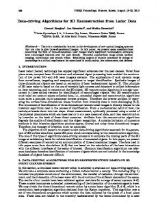
variance, using the sample variance, and credible intervals using the percentiles of the sample distribution. 5. Simulation Experiments 5.1. Illustration of monotonicity In this section the monotonicity method will be applied to the three resistivity distributions shown in Figure (1). The background resistivity is 1 Ωm and the inclusion 2 Ωm. In each the grounded reference electrode is to the right. The distributions, Barrier, C-Shape and Ring, cover a range of features designed to show the strengths and weaknesses of the method. Figure 1(d) shows typical noise-free data produced based on a 16 electrode system with equally spaced electrodes with equal width gaps, and using the reference protocol. Note that the resistivity distributions are defined on a generally coarse mesh. For the forward solution, however, note that there is a narrow ring at the outer edge and that a four-fold refinement of the displayed mesh is used. Both these result in a good level of accuracy in the forward solution.

Measured voltage (MeV)

3 2.5 2 1.5 1 0.5

(a)

(b)

(c)

0

50

100 150 Measurement Number

200

(d)

Figure 1: True inclusions: (a) Barrier, (b) C-Shape and (c) Ring, and (d) measurements from Barrier for a 16 electrode system. Using the mesh on which the resistivity distribution has been defined as the domain partition, for ease of comparison, produces the exterior sign index values shown in Figure 2(a). Again note that forward solution is performed on a much finer mesh. There is a wide spread of plausible inclusion pixels, and thresholding produces a good exterior set, Figure 2(b), including all true inclusion pixels but with several additional pixels

11

Bayesian reconstruction with monotonicity information

(a)

(b)

(c)

(d)

Figure 2: Barrier inclusion: (a) exterior sign index, sk (b) exterior sign index after thresholding, (c) interior sign index, tk , and (d) interior sign index after thresholding.

(a)

(b)

(c)

Figure 3: Sign index maps for noise-free data from 32 electrode systems, showing the interior set ΩInt (white), exterior set ΩExt (grey and white), and background (black). behind the inclusion. Similarly, the interior sign index and sign index map are shown in Figure(c,d) with the interior set exactly matching the true inclusion. The combination of the test results allows the shape of the inclusions to be approximately determined. Those pixels in the interior set are definitely in the inclusions, those not in the exterior set are definitely not in inclusions. It is not possible, however, to definitively assign the remaining pixels. Further modelling will be introduced before an attempt is made to assign these pixels. Applying the monotonicity to all the examples produces the three sign index maps shown in Figure 3. In each the black region is classified as background by the monotonicity test and the white as inclusion, whereas the grey region is unknown. All these are excellent, with no elements wrongly classified and only a few unclassified. It is only these unclassified, grey, elements which require further estimation.

12

Bayesian reconstruction with monotonicity information

(a)

(b)

(c)

(d)

Figure 4: Barrier truth: (a) Gauss-Newton reconstruction and then (b) posterior mean resistivity, (c) posterior standard deviation, and (d) posterior “probability of being inclusion”. 5.2. Conditional Bayesian estimation The proposed Bayesian model was fitted to low-noise data from the Barrier truth, using the sign map above, producing the results in Figure 4. Also shown is an all-element Gauss-Newton reconstruction. The detailed information from the monotonicity has produced a very good reconstruction, Figure 4(b). The elements hidden by the barrier have estimated resistivities close to those of the background. The posterior standard deviation, Figure 4(c), for the fixed elements is of course zero, and for the unassigned elements is roughly constant. The posterior estimates of “probability of being inclusion”, Figure 4(d), are highest for the elements truly part of the inclusion. These are all greater than a half, whilst the others are all substantially less than a half.

(a)

(b)

(c)

(d)

Figure 5: C-Shape truth: (a) Gauss-Newton reconstruction and then (b) posterior mean resistivity, (c) posterior standard deviation, and (d) posterior “probability of being inclusion”.

13

Bayesian reconstruction with monotonicity information

Figures 5 and 6 show similar sets of results for the C-Shaped and Ring truths. Both reconstructions clearly demonstrate that the unclassified elements are not part of the inclusion and the inclusion probabilities are unambiguous.

(a)

(b)

(c)

(d)

Figure 6: Ring truth: (a) Gauss-Newton reconstruction and then (b) posterior mean resistivity, (c) posterior standard deviation, and (d) posterior “probability of being inclusion”. The use of the monotonicity criterion to fix some resistivities has meant that, in these examples, as few as 10% of the image needs to be estimated in the MCMC algorithm. This gives an order of magnitude computational saving. Also, the accuracy and precision of the reconstruction results for all three resistivity distributions are excellent. 6. Concluding Remarks This paper has further investigated the framework for the inclusion of information derived from monotonicity into resistivity imaging though Bayesian modelling and MCMC algorithms.

These experiments provide evidence that this approach is

worthwhile with an impressive computational saving for the MCMC algorithm. For these 2D examples the extra calculations of the eigen calculations are insignificant, but would become substantial for large 3D problems. The Bayesian modelling and MCMC estimation algorithm provides a suitable approach to reconstructing the shape of a homogeneous resistivity inclusion in other homogeneous resistivity material. In most cases the number of pixels estimated in the MCMC algorithm is between about 10-30% of the total number of pixels in the

Bayesian reconstruction with monotonicity information

14

course mesh, hence there is a huge computational saving. For the estimated pixels, the algorithm provides flexible output in the form of standard deviations or posterior probabilities. Hence in summary, the combined approach provides an efficient and flexible method for imaging various two-phase materials. Acknowledgements: This work was partially support by the UK Engineering and Physical Sciences Research Council though grants GR/R22148/01 and GR/R64278/01. References [1] Aykroyd RG, Soleimani M, and Lionheart WRB (2004). Bayes-MCMC reconstruction from ERT data with prior constraints from resistance matrix monotonicity, In Proc: International Symposium on Industrial Process Tomography, Lodz, Poland. [2] Besag J, Green PJ, Higdon D and Mengersen K (1995). Bayesian computation and stochastic systems, Statistical Science, 10, 1-41. [3] Cheney, M, Isaacson,D, and Newell, JC (1999). Electrical impedance tomography. SIAM Review, 41, 85-101. [4] Kaipio JP, Kolehmainen V, Somersalo E and Vauhkonen M (2000). Statistical Inversion and Monte Carlo Sampling Methods in Electrical Impedance Tomography, Inverse Problems, 16, 1487-1522. [5] Kolehmainen V, Somersalo E, Vauhkonen M and Kaipio JP (1998). A Bayesian approach and total variation prior in 3D electrical impedance tomography, Proc. 20th Ann. Int. Conf. IEEE Eng Med. Biol. Soc. Hong Kong, 1028-31. [6] Liu, JS (2001). Monte Carlo Strategies in Scientific Computing, Springer-Verlag:

Berlin,

Heidelberg. [7] Nicholls GK and Fox C (1998) Prior modelling and posterior sampling in impedance imaging, Proc. SPIE, 3459, 116-127. [8] Somersalo E, Cheney M and Isaacson D (1992), Existence and Uniqueness for Electrode Models for Electric Current Computed Tomography, SIAM. J Appl Math, 52, 1023-1040. [9] Tamburrino A and Rubinacci G (2002). A new non-iterative inversion method for electrical resistance tomography. Inverse Problems, 18, 1809-1829 [10] Tamburrino A, Rubinacci G, Soleimani M, Lionheart WRB (2003). A Noniterative Inversion Method for Electrical Resistance, Capacitance and Inductance Tomography for Two Phase Materials, In Proc. 3rd World Congress on Industrial Process Tomography, Canada, pp. 233-238. [11] Vauhkonen M, Lionheart WRB, Heikkinen LM, Vauhkonen PJ, and Kaipio JP (2001). A MATLAB Package for the EIDORS Project to Reconstruct Two-dimensional EIT Images, Physiological Measurements, 22, 107-111.

Bayesian reconstruction with monotonicity information

15

[12] West RM, Aykroyd RG, Meng S and Williams RA (2004). Markov Chain Monte Carlo Techniques and Spatial-Temporal Modelling for Medical EIT, Physiological Measurements, 25, 181-194. [13] West RM, Meng S, Aykroyd RG and Williams RA (2005). Spatial-temporal Modelling for EIT of a Mixing Process. Review of Scientific Instruments, To appear. [14] Winkler, G (2003). Image Analysis, Random Fields and Markov Chain Monte Carlo: Mathematical Introduction (2nd Ed.), Springer-Verlag: Berlin.

A