Confidence Intervals for the Overall Effect Size in ... - Semantic Scholar

Psychological Methods 2008, Vol. 13, No. 1, 31– 48

Copyright 2008 by the American Psychological Association 1082-989X/08/$12.00 DOI: 10.1037/1082-989X.13.1.31

Confidence Intervals for the Overall Effect Size in Random-Effects Meta-Analysis Julio Sańchez-Meca and Fulgencio Marıń-Martıńez University of Murcia One of the main objectives in meta-analysis is to estimate the overall effect size by calculating a confidence interval (CI). The usual procedure consists of assuming a standard normal distribution and a sampling variance defined as the inverse of the sum of the estimated weights of the effect sizes. But this procedure does not take into account the uncertainty due to the fact that the heterogeneity variance (␶2) and the within-study variances have to be estimated, leading to CIs that are too narrow with the consequence that the actual coverage probability is smaller than the nominal confidence level. In this article, the performances of 3 alternatives to the standard CI procedure are examined under a random-effects model and 8 different ␶2 estimators to estimate the weights: the t distribution CI, the weighted variance CI (with an improved variance), and the quantile approximation method (recently proposed). The results of a Monte Carlo simulation showed that the weighted variance CI outperformed the other methods regardless of the ␶2 estimator, the value of ␶2, the number of studies, and the sample size. Keywords: meta-analysis, random-effects model, confidence intervals, heterogeneity variance, standardized mean difference

dependent variable is dichotomous or has been dichotomized, then effect-size indices such as an odds ratio (or its log transformation), a risk ratio (or its log transformation), or a risk difference can be applied (Egger, Smith, & Altman, 2001; Haddock, Rindskopf, & Shadish, 1998; SańchezMeca, Marıń-Martıńez, & Chacoń-Moscoso, 2003). If all of the variables are continuous, then an effect-size index from the r family can be applied, such as the Pearson correlation coefficient or its Fisher’s Z transformation (Hunter & Schmidt, 2004; Rosenthal, 1991; Rosenthal, Rosnow, & Rubin, 2000). In general, the statistical analysis usually applied in metaanalysis has three main objectives: (a) to estimate the overall effect size of the population to which the studies pertain; (b) to assess if the heterogeneity found among the effect estimates can be explained by chance alone or if, on the contrary, the individual studies exhibited true heterogeneity, that is, variability produced by real differences among the population effect sizes; and, (c) if heterogeneity cannot be explained by sampling error alone, to search for study characteristics that could operate as moderator variables of the effect estimates. Our focus in this article was the first objective, that is, to estimate the population effect size. To estimate the population effect size from a set of individual studies, an average of the effect estimates is calculated by weighting each one of them by its inverse variance, and a confidence interval (CI) is thus obtained

Meta-analysis is a research methodology that aims to integrate, by applying statistical methods, the results of a set of empirical studies about a given topic. To accomplish its purpose, a meta-analysis requires a thorough search of the relevant studies, and the results of each individual study have to be translated into the same metric (Cooper, 1998; Lipsey & Wilson, 2001). Depending on such study characteristics as the design type and how the variables implied were measured, the meta-analyst has to select one of the different effect-size indices and apply it to all of the studies of the meta-analysis (Grissom & Kim, 2005). So, when the dependent variable is continuous and the purpose of each study is to compare the performance between two groups, the standardized mean difference is the most usual effectsize index (Cooper, 1998; Hedges & Olkin, 1985). If the

Julio Sańchez-Meca and Fulgencio Marıń-Martıńez, Department of Basic Psychology and Methodology, Faculty of Psychology, Espinardo Campus, University of Murcia, Murcia, Spain. This article was supported by a grant from the Ministerio de Educacioń y Ciencia of the Spanish Government and by Fondo Europeo de Desarrollo Regional funds for Project No. SEJ200407278/PSIC. Correspondence concerning this article should be addressed to Julio Sańchez-Meca, Department of Basic Psychology and Methodology, Faculty of Psychology, Espinardo Campus, University of Murcia, 30100-Murcia, Spain. E-mail: [email protected] 31

´ NCHEZ-MECA AND MARIŃ-MARTIŃEZ SA

32

around it. Most of the effect-size indices usually applied in meta-analysis are approximately normally distributed and their sampling variances can be easily estimated by simple algebraic formulas (Fleiss, 1994; Rosenthal, 1994; Shadish & Haddock, 1994). As a consequence, meta-analyses typically calculate a CI for the overall effect size assuming a standard normal distribution to estimate the population effect size, with the sampling variance estimated as the inverse of the sum of the estimated weights. This procedure performs well when the effect estimates obtained in the studies differ among themselves only by sampling error, that is, when the effect estimates assume a fixed-effects model or the heterogeneity variance is small. However, when the underlying statistical model in the meta-analysis is a random-effects model, the empirical coverage probability of this CI for the average effect size systematically underestimates the nominal confidence level (Brockwell & Gordon, 2001, 2007; Sidik & Jonkman, 2002). In recent years, the random-effects model has been considered the most realistic statistical model in meta-analysis (Field, 2001, 2003; Hedges & Vevea, 1998; Overton, 1998; Raudenbush, 1994). Therefore, to obtain CIs for the overall effect size with a good coverage probability is an important issue. Our purpose in writing this article was to compare the performances of three alternative CI procedures with that based on the standard normal distribution to estimate the overall effect size when the underlying statistical model is a random-effects model. Moreover, we also examined whether different heterogeneity variance estimators affect the coverage probability of the CIs for the overall effect size. Thus, we started from the idea that a good CI procedure to estimate an overall effect size should offer good coverage, that is, close to nominal, and the coverage should not be affected by the value of the heterogeneity variance, by the heterogeneity variance estimator used in the metaanalysis, or by the number of studies. The four CI procedures analyzed here are very simple to calculate, not requiring iterative numerical computation. Other methods of obtaining CIs that are computationally more complex and are not addressed here are those of Biggerstaff and Tweedie (1997) or the profile likelihood method of Hardy and Thompson (1996).

The Random-Effects Model Let k be a set of independent empirical studies about a given topic and ␪ˆ i be the effect-size estimate obtained in the ith study. The underlying statistical model can be represented as ␪ˆ i ⫽ ␪ i ⫹ e i,

(1)

where ei is the sampling error of ␪ˆ i . Usually ei is assumed to be normally distributed, ei ⬃ N(0, ␴ 2i ), with ␴ 2i being the

within-study variance. The random-effects model assumes that each single study estimates its own parametric effect size ␪i and, as a consequence, ␪i constitutes a random variable with mean ␮ and between-studies variance ␶2. The between-studies variance, also named heterogeneity variance, represents the variability between the estimated effect sizes due not to within-study sampling error but to true heterogeneity among the studies. In other words, the heterogeneity variance represents the variability produced by the influence of the differential characteristics of the studies, such as the design quality, the characteristics of the subjects in the samples, or differences in the program implementation. This implies that each parametric effect size, ␪i, can be decomposed as ␪ i ⫽ ␮ ⫹ ε i,

(2)

with εi representing the difference between the parametric effect size of the ith study, ␪i, and the parametric mean, ␮. The errors εi are usually assumed to be normally distributed, with heterogeneity variance ␶2, εi ⬃ N(0, ␶2). It is also assumed that the errors ei and εi are independent. So, combining Equations 1 and 2 enables us to formulate the random-effects model as ␪ˆ i ⫽ ␮ ⫹ e i ⫹ ε i,

(3)

and, as a consequence, the estimated effect sizes ␪ˆ i are assumed to be normally distributed with mean ␮ and variance ␶ 2 ⫹ ␴ 2i , ␪ˆ i ⬃N(␮, ␶ 2 ⫹ ␴ 2i ). When there is not true heterogeneity, then the betweenstudies variance is zero, ␶2 ⫽ 0, and the random-effects model becomes a fixed-effects model, that is, all of the individual studies estimate the same parametric effect size ␪1 ⫽ ␪2 ⫽ . . . ⫽ ␪k ⫽ ␮ ⫽ ␪. In this case, Equation 3 simplifies to ␪ˆ i ⫽ ␪ ⫹ ei , and the effect estimates ␪ˆ i are assumed to be normally distributed with mean ␪ and variance ␴ 2i , ␪ˆ i ⬃N(␪, ␴ 2i ). Thus, the fixed-effects model can be considered a particular case of the random-effects model when differences among the effect estimates are only due to sampling error. Both models, those of random and fixed effects, can be extended to include moderator variables. They are not presented here, however, as our purpose is to compare the performance of different procedures to calculate a CI around the overall effect size.

CIs for the Overall Effect Size One of the main objectives in meta-analysis is to obtain an average effect-size estimate from a set of independent effect-size estimates and to calculate a CI around it to estimate the parametric effect size, ␮. In practice, the studies included in a meta-analysis have different sample sizes and, as a consequence, the precision of the effect-size estimates varies among them. A good estimator of the mean

CONFIDENCE INTERVALS IN META-ANALYSIS

parametric effect size should take into account the precision of the effect estimates. The most usual procedure to achieve this objective consists of weighting each effect-size estimate by its inverse variance. In a random-effects model, the uniformly minimum variance unbiased estimator (UMVU) of ␮ is given by

冘 w ␪ˆ ⫽ 冘w

i i

␮ˆ UMVU

i

(4)

i

i

(Viechtbauer, 2005), with wi being the optimal or true weights wi ⫽ 1/共␶2 ⫹ ␴2i 兲. The sampling variance of ␮ˆ UMVU is given by V共␮ˆ UMVU兲 ⫽

1 . wi

冘

(5)

i

If, in a meta-analysis, the population sampling variance of each study, ␴ 2i , and the population heterogeneity variance, ␶2, are known, then ␮ˆ UMVU can be calculated and, as it is asymptotically normally distributed, a 100(1 ⫺ ␣)% CI assuming a standard normal distribution can be calculated by

冑

␮ˆ UMVU ⫾ z1 ⫺ ␣/ 2 V共␮ˆ UMVU),

(6)

where z1⫺␣/2 is the 100(1 ⫺ ␣/2) percentile of the standard normal distribution, ␣ being the significance level.

The z Distribution CI In practice, neither the parametric heterogeneity variance, ␶2, nor the parametric sampling variances of the single studies, ␴ 2i , are known. Therefore, they have to be estimated from the data reported in the studies. This means that Equation 6 cannot ever be applied. For most of the effectsize indices usually applied in meta-analysis, unbiased estimators of the sampling variance, ␴ˆ 2i , have been derived, and several estimators can be found in the literature to estimate the heterogeneity variance in a meta-analysis, ␶ˆ 2 (Sidik & Jonkman, 2007; Viechtbauer, 2005). Once we have an unbiased sampling variance estimator, ␴ˆ 2i , to be applied in each study and a heterogeneity variance estimator, ␶ˆ 2, the optimal weights, wi, can be estimated by wî ⫽ 1/共␶ˆ 2 ⫹ ␴ˆ 2i 兲. Therefore, the formula for estimating the parametric mean effect size, ␮, in meta-analysis is given by

冘 wˆ ␪ˆ ␮ˆ ⫽ 冘 wˆ , i i

i

i

i

(7)

33

and its sampling variance is usually estimated as Vˆ 共␮ˆ 兲 ⫽

1

冘 wˆ .

(8)

i

i

The typical procedure to calculate a CI around an overall effect size assumes a standard normal distribution and estimates the sampling variance of ␮ˆ by Equation 8. Here we refer to this procedure as the z distribution CI, which is obtained by ␮ˆ ⫾ z1 ⫺ ␣/ 2 冑Vˆ共␮ˆ 兲.

(9)

However, this procedure does not take into account the uncertainty produced by the fact that the within-study and the between-studies variances have to be estimated (Biggerstaff & Tweedie, 1997). As Sidik and Jonkman (2003) have contended, “The normality assumption for ␮ˆ is not strictly true in practice (nor is Vˆ (␮ˆ ) the true variance), because the wˆ i values are estimates. Nonetheless, this is the commonly used practice for constructing CIs” (p. 1196). The main consequence of assuming a standard normal distribution to obtain a CI for ␮ˆ with Equation 9 is that its actual coverage probability is smaller than the nominal confidence level, the width of the CI being too narrow. As Viechtbauer (2005) has shown, estimating the optimal weights, wi, using unbiased estimates of ␶2 and ␴ 2i , results in an estimate of the sampling variance of ␮ˆ that is negatively biased. As a consequence of this negative bias, the sampling variance of ␮ˆ will be underestimated on average, and researchers will attribute unwarranted precision to their estimate of ␮. (p. 263)

Moreover, several Monte Carlo studies have shown that the underestimation of the nominal confidence level with the z distribution CI is more severe as the between-studies variance increases and as the number of studies decreases. The z distribution CI only presents good coverage probability in meta-analyses with a large number of studies and very little or zero heterogeneity variance (Brockwell & Gordon, 2001, 2007; Follmann & Proschan, 1999; Hartung & Makambi, 2003; Makambi, 2004; Sidik & Jonkman, 2002, 2003, 2005, 2006).

The t Distribution CI To solve the problems of coverage probability with the z distribution CI, it has been proposed in the literature (Follmann & Proschan, 1999; Hartung & Makambi, 2002) to assume a Student t reference distribution with k – 1 degrees of freedom, instead of the standard normal distribution, and to estimate the sampling variance of ␮ˆ in Equation 8 with ␮ˆ ⫾ tk ⫺ 1,1 ⫺ ␣/ 2 冑Vˆ共␮ˆ 兲,

(10)


34

with tk⫺1, 1⫺␣/2 being the 100(1 ⫺ ␣/2) percentile of the t distribution with k – 1 degrees of freedom. Here we refer to this procedure as the t distribution CI. Using a t distribution produces CIs that are wider than those of the standard normal distribution, in particular for meta-analyses with a small number of studies, and, consequently, this should improve the coverage probability, as Follmann and Proschan (1999) have found.

The Weighted Variance CI One procedure that has not yet widely been used in meta-analysis is that proposed by Hartung (1999), which consists of calculating a CI for the overall effect size assuming a Student t distribution with k – 1 degrees of freedom and estimating the sampling variance of ␮ˆ with a weighted extension of the usual formula, Vˆ w(␮ˆ ):

冘 wˆ 共␪ˆ ⫺ ␮ˆ 兲 Vˆ 共␮ˆ 兲 ⫽ , 共k ⫺ 1兲冘 wˆ 2

i

i

i

w

(11)

␮ˆ ⫾ b1 ⫺ ␣/ 2 冑Vˆ共␮ˆ 兲

(13)

(Brockwell & Gordon, 2007, p. 4538), where Vˆ (␮ˆ ) is the usual formula to estimate the sampling variance of ␮ˆ , defined in Equation 8, and b1⫺␣/2 is the 100(1 ⫺ ␣/2)% percentile of the distribution of M empirically approached by Monte Carlo simulation. Unlike the other three procedures for calculating a CI for the overall effect size in a random-effects meta-analysis, the critical values in the Brockwell and Gordon (2007) method are obtained by simulating thousands of meta-analyses from a random-effects model and varying the number of studies between 2 and 30 and the heterogeneity variance between 0 and 0.5. The effect-size index that they used in the simulations was the log odds ratio, as it is a very common effect estimator in the medical literature. Once Brockwell and Gordon (2007) obtained the observed values for the quantiles 100(␣/2)% and 100(1 ⫺ ␣/2)% of the M statistic, they adjusted a regression equation for the quantiles as a function of the number of studies, k:

i

i

where wî ⫽ 1/共␶ˆ 2 ⫹ ␴ˆ 兲 and ␮ˆ is the overall effect size defined in Equation 7 assuming a random-effects model. It can be shown that the statistic (␮ˆ ⫺ ␮)/ 公Vˆ w(␮ˆ ) is approximately distributed as a t distribution with k – 1 degrees of freedom (Hartung, 1999; Sidik & Jonkman, 2002). Therefore, a CI around the overall effect size can be computed by 2 i

冑

␮ˆ ⫾ tk ⫺ 1,1 ⫺ ␣/ 2 Vˆw(␮ˆ ).

(12)

Following Sidik and Jonkman (2003, 2006), here we refer to this procedure as the weighted variance CI. Previous simulations seem to offer good coverage of this procedure when the effect-size index is the log odds ratio (Makambi, 2004; Sidik & Jonkman, 2002, 2006), the standardized mean difference (Sidik & Jonkman, 2003), and the unstandardized mean difference and the risk difference (Hartung & Makambi, 2003). In particular, the weighted variance CI offers a better coverage probability than the z distribution CI except when the between-studies variance is zero, ␶2 ⫽ 0 (Hartung, 1999; Hartung & Makambi, 2003; Sidik & Jonkman, 2002, 2003).

The Quantile Approximation (QA) Method The fourth method of calculating a CI for the overall effect size that is included in this study has been recently proposed by Brockwell and Gordon (2007). The method consists of approximating, by means of intensive computation, the quantiles of the distribution of the statistic M ⫽ 共␮ˆ ⫺ ␮兲/ 冑Vˆ共␮ˆ 兲 and then using the 100(1 ⫺ ␣/2)% percentile of the M distribution to calculate a CI for the overall effect size by

b 1⫺␣/ 2 ⫽ 2.061 ⫹

4.902 0.756 0.958 ⫹ ⫺ k ln共k兲冑k

(14)

(Brockwell & Gordon, 2007, p. 4538). Thus, the critical values, b1⫺␣/2, to be used in the CI formula (Equation 13) of Brockwell and Gordon (2007) are estimated from Equation 14. For example, if a meta-analysis has k ⫽ 10 studies, then the corresponding critical value for a 95% nominal confidence level is b.975 ⫽ 2.374. Here we refer to this procedure as the QA method. Brockwell and Gordon (2007) have found a better performance of this procedure than those of the z and t distribution CIs, using the DerSimonian and Laird (1986) estimator of the heterogeneity variance, but they did not compare the QA method with the weighted variance CI.

Heterogeneity Variance Estimators To calculate a CI around the overall effect size in a meta-analysis where a random-effects model is assumed, an estimate of the heterogeneity variance is needed. Although meta-analyses typically use the heterogeneity variance estimator proposed by DerSimonian and Laird (1986), alternative estimators have been proposed that seem to offer better properties than the usual estimator. Some of the alternatives are based on noniterative estimation procedures, whereas others require iterative computations. Different heterogeneity variance estimators differ in respect to such statistical properties as bias and mean square error (Sidik & Jonkman, 2007; Viechtbauer, 2005, 2007), and an issue that has not yet been widely studied is whether the selection of the heterogeneity variance estimator has an effect on the performance of different CIs for the overall


35

effect size. Next, we present formulas to calculate eight different heterogeneity variance estimators that could be used to obtain CIs for the overall effect size under a random-effects model.

2 As ␶ˆ HE is not a nonnegative heterogeneity variance estima2 tor, it has to be truncated to zero when ␶ˆ HE ⬍ 0.

Hunter and Schmidt (HS) Estimator

The heterogeneity variance estimator usually applied in the meta-analytic literature is that proposed by DerSimonian and Laird’s (1986) estimator, which is based on the moments method, consists of estimating the population heterogeneity variance by

Hunter and Schmidt (1990, pp. 285–286; see also Hunter & Schmidt, 2004, pp. 287–288) proposed to estimate the heterogeneity variance by calculating the difference between the total variance of the effect estimates and an average of the estimated within-study variances, ␴ˆ 2i . A simplified formula of this estimator is given by 2 ␶ˆ HS ⫽

Q⫺k , wˆFE i

冘

(15)

i

⫽ 1/␴ˆ 2i is the inverse variance of the ith study where wˆFE i assuming a fixed-effects model, with ␴ˆ 2i being the withinstudy variance estimate for the ith study. Q is the heterogeneity statistic usually applied to test the homogeneity hypothesis (Hedges & Olkin, 1985): Q⫽

冘

wˆ 共␪ˆ i ⫺ ␮ˆ FE兲2 , FE i

(16)

DerSimonian and Laird (DL) Estimator

2 ⫽ ␶ˆ DL

Q ⫺ 共k ⫺ 1兲 , c

(20)

where Q is the heterogeneity statistic defined in Equation 16 and c is given by

冘共wˆ 兲 c ⫽ 冘 wˆ ⫺ 冘 wˆ . FE 2 i

i

FE i

(21)

FE i

i

i

2 2 When Q ⬍ (k – 1), then ␶ˆ DL is negative and, like ␶ˆ HS and 2 ␶ˆ HE, it has to be truncated to zero.

i

with ␮ˆ FE being the mean effect size, assuming a fixedeffects model; that is,

冘 wˆ ␪ˆ ⫽ 冘 wˆ . FE i i

i

␮ˆ FE

(17)

FE i

i

2 If Q ⬍ k, then ␶ˆ HS is negative and, as a consequence, it has to be truncated to zero.

Malzahn, Bo¨hning, and Holling (MBH) Estimator Malzahn, Bo¨hning, and Holling (2000) proposed a momentbased nonparametric estimator of the population heterogeneity variance specifically designed to be used only with the standardized mean difference, d. It is also based on the difference of an estimate of the total variance of the d indices and an estimate of the average within-study variance of the d indices. It is obtained by

冘共1 ⫺ ␸ 兲共␪ˆ ⫺ ␮ˆ i

Hedges (HE) Estimator

2 ␶ˆ MBH ⫽

The HE estimator of the population heterogeneity variance consists of calculating the difference between an unweighted estimate of the total variance of the effect sizes and an unweighted estimate of the average within-study variance (Hedges, 1983, p. 391; see also Hedges & Olkin, 1985, p. 194):

冘共␪ˆ ⫺ ␮ˆ i

2 ⫽ ␶ˆ HE

兲2

UW

i

⫺

k⫺1

1 k

冘 ␴ˆ , 2 i

(18)

i

where ␮ˆ UW is an unweighted mean of the effect sizes

冘 ␪ˆ

i

␮ˆ UW ⫽

i

k

.

(19)

i

i

k⫺1

兲2

FE

⫺

1 k

冘冉n Nn 冊 ⫺ 1k 冘 ␸ ␪ˆ i

i

Ei Ci

2 i i

i

(22) (Malzahn et al., 2000, p. 622; see also Malzahn, 2003), with Ni ⫽ nEi ⫹ nCi being the total sample size of the ith study; ␮ˆ FE was defined in Equation 17, ␪ˆ i is the d index for the ith study, and ␸i is given by ␸i ⫽ 1 ⫺

Ni ⫺ 4 , 关c共m i兲兴 2共N i ⫺ 2兲

(23)

with c(mi) being the correction factor of the d index for small sample sizes, defined in Equation 33. Applications of this estimator are limited to meta-analyses where the effect2 size index is the d index. When ␶ˆ MBH has a negative value, it is truncated to zero.


36

Hartung and Makambi (HM) Estimator Hartung and Makambi (2003; see also Makambi, 2004) proposed a positive heterogeneity variance estimator that attempts to improve the performance of the usual DL estimator. A simplified formula of this estimator is given by ␶ˆ

2 HM

Q2 , ⫽ 关2共k ⫺ 1兲 ⫹ Q兴c

(24)

Sidik and Jonkman (SJ) Estimator Another estimator of the heterogeneity variance in metaanalysis, recently proposed by Sidik and Jonkman (2005), also yields nonnegative values. The SJ estimator is a simple noniterative estimator of the heterogeneity variance that is based on a reparametrization of the total variance in the effect estimates, ␪ˆ i . It is obtained by

冘

⫺1 i

vˆ 共␪ˆ i ⫺ ␮ˆ vˆ兲2

i

␶ˆ ⫽

,

k⫺1

(25)

(Sidik & Jonkman, 2005, p. 371; see also Sidik & Jonkman, 2007), where vˆ i ⫽ ri ⫹ 1, ri ⫽ ␴ˆ 2i /␶ˆ 02 , and ␶ˆ 20 is an initial estimate of the heterogeneity variance, which can be defined, for example, as

冘共␪ˆ ⫺ ␮ˆ i

UW

i

␶ˆ 02 ⫽

兲2 ,

k

(26)

␮ˆ UW being the unweighted mean of the effect estimates, defined in Equation 19, and ␮ˆ vˆ is given by

冘 ␮ˆ ⫽ 冘 vˆ

⫺1 i i

vˆ ␪ˆ

i

⫺1 i

vˆ

冘 wˆ 关共␪ˆ ⫺ ␮ˆ ⫽ 冘 wˆ 2 i

with Q and c defined in Equations 16 and 21, respectively. An advantage of this estimator is that it cannot yield negative values.

2 SJ

2001; DerSimonian & Laird, 1986; Hardy & Thompson, 1996; Raudenbush & Bryk, 1985). For a specified convergence criterion, the formula that enables us to estimate the population heterogeneity variance by maximum likelihood under a random-effects model is given by

2 ␶ˆ ML

i

i

(27)

i

Thus, in the SJ estimator, the weights are a function not only of the within-study variances but also of a crude estimate of the heterogeneity variance. Although other initial ␶ˆ 20 estimates can be proposed, we used the one originally recommended by Sidik and Jonkman (2005).

Maximum Likelihood (ML) Estimator The six heterogeneity variance estimators presented above are noniterative. Two iterative estimators proposed in the meta-analytic literature to estimate the heterogeneity variance are based on maximum likelihood and restricted maximum likelihood estimation (Brockwell & Gordon,

(28)

2 i

i

(Sidik & Jonkman, 2007; Viechtbauer, 2005, p. 268), with wî ⫽ 1/共␶ˆ 2 ⫹ ␴ˆ 2i 兲, where ␶ˆ 2 is initially estimated by any of the noniterative estimators of the heterogeneity variance or setting ␶ˆ 2 ⫽ 0 and ␮ˆ ML is given by

冘 wˆ ␪ˆ ⫽ 冘 wˆ . i i

␮ˆ ML

i

(29)

i

i

In each iteration of Equations 28 and 29, the estimate of ␶2 has to be checked to avoid having negative values truncating it to zero. Convergence is usually achieved within fewer than 10 iterations.

Restricted Maximum Likelihood Estimator The second iterative estimator of the heterogeneity variance in a random-effects model is based on restricted maximum likelihood estimation (REML). The REML estimator of ␶2 compensates for the negative bias of the ML estimator by applying a linear combination of the effect sizes. The REML estimator of the heterogeneity variance is given by

冘 wˆ 关共␪ˆ ⫺ ␮ˆ ⫽ 冘 wˆ 2 i

2 ␶ˆ REML

i

兲2 ⫺ ␴ˆ 2i 兴

ML

i

2 i

i

.

兲2 ⫺ ␴ˆ 2i 兴

ML

⫹

1 wî

冘

(30)

i

(Viechtbauer, 2005, p. 269). The iterative procedure is 2 similar to that of the ML estimator. When ␶ˆ REML ⬍ 0, it is truncated to zero to avoid negative values.

An Example To illustrate the calculations and the extent to which different CI procedures and heterogeneity variance estimators can yield differences in the interval estimations of the overall effect size, we have selected the example cited in Hedges and Olkin (1985, p. 25), composed of the results of 10 studies on the effectiveness of open versus traditional education on student creativity. The effect-size index applied was the standardized mean difference, d. Table 1 presents the d value, di; the sample size; and the estimated

CONFIDENCE INTERVALS IN META-ANALYSIS Table 1 Effect Estimates, Sample Sizes, and Estimated Within-Study Variances for the Example Data di

nEi ⫽ nCi

␴ˆ 2i

⫺0.581 0.530 0.771 1.031 0.553 0.295 0.078 0.573 ⫺0.176 ⫺0.232

90 40 36 20 22 10 10 10 39 50

0.023 0.052 0.060 0.113 0.094 0.202 0.200 0.208 0.051 0.040

Study 1 2 3 4 5 6 7 8 9 10

within-study variance, ␴ˆ 2i , for each study. In total, we calculated 32 CIs assuming a random-effects model, resulting from the combination of four CI procedures (z distribution CI with Equation 9, t distribution CI with Equation 10, weighted variance CI with Equation 12, and QA method with Equation 13) with eight heterogeneity variance estimators (Equations 15, 18, 20, 22, 24, 25, 28, and 30). Table 2 shows the results obtained with the different CI procedures. A first interesting result is that the standard errors of ␮ˆ obtained with the usual formula, 公Vˆ (␮ˆ ), were more dependent on the ␶2 estimator than were those calculated with the weighted sampling variance, 公Vˆ w(␮ˆ ). In particular, standard errors obtained from the weighted variance, 公Vˆ w(␮ˆ ), varied from 0.166 to 0.169, whereas standard errors from the usual variance, 公Vˆ (␮ˆ ), ranged from 0.154 to 0.192; that is, the range for 公Vˆ (␮ˆ ) was about 12 times larger than that of 公Vˆ w(␮ˆ ). Moreover, a positive relationship was found between the standard errors from the usual formula and the ␶2 estimates. However, the overall effect estimates, ␮ˆ , varied as a function of the ␶2 estimator from 0.230 to 0.251. As expected, for common values of ␶ˆ 2, the width of the CIs based on the z distribution was narrower

37

than the widths obtained with the t distribution CI, the weighted variance CI, and the QA method (except for the DL heterogeneity variance estimator). On average, the widths of the CIs based on the z distribution, t distribution, weighted variance, and QA method were 0.680, 0.784, 0.758, and 0.823, respectively. The width of the CI obtained with the QA method was slightly larger than that of the t distribution CI because of the different critical value used: 2.374 for b1⫺␣/2 versus 2.262 for tk⫺1,1⫺␣/2. Furthermore, the width of the CIs obtained with the weighted variance procedure through the different heterogeneity variance estimators varied about 12 times less (SD ⫽ 0.004) than those obtained with z distribution, t distribution, and QA method CIs (SDs ⫽ 0.046, 0.053, and 0.055, respectively). Therefore, the weighted variance CI seems to be less dependent on the ␶2 estimator than are the other three CI procedures. This example illustrates how the selection of the ␶2 estimator and the procedure for calculating a CI for the overall effect size can affect the results.

Monte Carlo Study Although several Monte Carlo studies have compared the coverage probability of the usual CI and that proposed by Hartung (1999) under a random-effects model, the extent to which different heterogeneity variance estimators can affect their performance has not yet been widely examined. In previous studies, the usual DL estimator was used (Sidik & Jonkman, 2002, 2006), and its influence on the coverage probability has been compared with one (Hartung & Makambi, 2003; Makambi, 2004) or two (Sidik & Jonkman, 2003) alternative estimators of the heterogeneity variance only in some cases. Moreover, a comparison of the performance of the four CI procedures has not yet been carried out. However, only one of these simulation studies focused on the standardized mean difference as the effect-size index (Sidik & Jonkman, 2003). Finally, previous simulation stud-

Table 2 Results Based on Different Heterogeneity Variance Estimators and Confidence Interval (CI) Procedures for the Example Data ␶ estimator

␶ˆ

HS HE DL MBH HM SJ ML REML

0.229 0.148 0.277 0.204 0.248 0.199 0.200 0.220

2

2

Width of the 95% CI for ␮

␮ˆ

冑Vˆ (␮ˆ )

冑Vˆw (␮ˆ )

z distribution

t distribution

Weighted variance

QA method

0.245 0.230 0.251 0.235 0.248 0.241 0.241 0.244

0.179 0.154 0.192 0.160 0.184 0.170 0.170 0.176

0.167 0.169 0.166 0.169 0.168 0.168 0.168 0.167

0.702 0.603 0.754 0.629 0.723 0.667 0.668 0.691

0.810 0.696 0.871 0.725 0.834 0.770 0.771 0.798

0.756 0.766 0.752 0.763 0.754 0.759 0.759 0.757

0.850 0.730 0.914 0.761 0.875 0.808 0.809 0.837

Note. CI ⫽ confidence interval; HS ⫽ Hunter and Schmidt estimator; HE ⫽ Hedges estimator; DL ⫽ DerSimonian and Laird estimator; MBH ⫽ Malzahn, Bo¨hning, and Holling estimator; HM ⫽ Hartung and Makambi estimator; SJ ⫽ Sidik and Jonkman estimator; ML ⫽ maximum likelihood estimator; REML ⫽ restricted maximum likelihood estimator.

38


ies have not manipulated the parametric mean effect size, ␮, because it is expected that CIs calculated from z and t distributions should be invariant to a location shift (Brockwell & Gordon, 2001; Sidik & Jonkman, 2005). However, as the weights used in the calculations of the overall effect size, ␮ˆ , and of the variances for ␮ˆ are estimated weights, wˆ i , and not the true or “correct” weights, wi, changes in ␮ could affect the coverage probability of the CIs. This is of particular interest when the effect-size index is the standardized mean difference, as the within-study variance of each study is a function of the parametric effect size, ␦i. Therefore, we carried out Monte Carlo simulations to determine whether (a) different assumptions about the underlying sampling distribution of the overall effect size (standard normal distribution, Student t distribution, and quantile approximation); (b) different estimators of the sampling variance of ␮ˆ (the usual or the weighted sampling variance); (c) different heterogeneity variance estimators; and (d) changes in the parametric mean effect size, ␮, can affect the coverage probability when constructing a CI around an overall standardized mean difference in a random-effects meta-analysis. Moreover, the performance of the different CI procedures was examined as a function of such factors as the number of studies, the value of the heterogeneity variance, and the average sample size. Finally, for comparison purposes, the four CI procedures were also calculated from the optimal or correct weights, wi. From the results of previous research, we had several expectations. First, in respect to the z distribution CI, we expected to find (a) a good adjustment of the empirical coverage probability to the nominal confidence level only when ␶2 ⫽ 0 and (b) an empirical coverage probability that becomes increasingly less than the nominal coverage probability as ␶2 increases and the number of studies, k, decreases. Second, the t distribution CI should offer better coverage than that based on the standard normal distribution (Follmann & Proschan, 1999). In respect to the weighted variance CI, we expected to obtain a closer approximation to the nominal coverage probability by the actual coverage probability regardless of the values of ␶2 and k (Makambi, 2004; Sidik & Jonkman, 2003). The QA method should offer better coverage as ␶2 and the number of studies increase. Furthermore, Sidik and Jonkman (2003) found that the coverage probability of the weighted variance CI is less affected by the ␶2 estimator than is that based on the standard normal distribution. In particular, they showed this finding with three ␶2 estimators (DL, MBH, and HE estimators). We expected to generalize this finding to the eight ␶2 estimators examined here and, thus, to show the higher robustness to changes in the ␶2 estimator of the weighted variance CI, in comparison with that of the z distribution, t distribution, and QA method CIs. Finally, as expected from the statistical theory, the z distribution CI applied on the

optimal or correct weights should offer the best adjustment to the nominal level. In our simulation study, the effect-size index was the standardized mean difference. To simulate each individual study, we defined a two-group design (e.g., experimental vs. 2 control) and a continuous outcome. Define ␴w as the withi in-study variance of observations for study i. Under a random-effects model, the population standardized mean difference for each study, ␦i, was defined as ␦i ⫽

␮ Ei ⫺ ␮Ci , ␴wi

(31)

where ␮Ei and ␮Ci were the population means for the experimental and the control groups in the ith study and ␴wi was the common population standard deviation of the ith study. For each study, normal distributions in the experimental and the control groups were assumed for the continuous outcome. The population standardized mean differences, ␦i, were normally distributed with mean ␮ and variance ␶2, that is, ␦i ⬃ N(␮, ␶2). Here, ␦i and ␮ correspond with ␪i and ␮, respectively, in previous equations. From the normal distribution of ␦i values, collections of k independent studies were randomly generated to simulate a meta-analysis. Once a ␦i value was randomly selected, the ith study was simulated by generating two normal distributions (for the experimental and control groups) with means of ␮Ei ⫽ ␦i and ␮Ci ⫽ 0 and common standard deviation ␴wi ⫽ 1. Then, pairs of independent samples (experimental and control) were randomly selected from the two distributions of the continuous outcome with sample sizes nEi ⫽ nCi, and the means, y៮ Ei and y៮ Ci , and the standard deviations, SEi and SCi, were calculated. Thus, for the ith study, ␦i was estimated by the d index d i ⫽ c共m i兲

y៮ Ei ⫺ y៮ Ci , Si

(32)

where c(mi) is a correction factor for small sample sizes that is approached by c共m i兲 ⫽ 1 ⫺

3 4共n Ei ⫹ nCi 兲 ⫺ 9

(33)

(Hedges & Olkin, 1985), and Si is the pooled within-study standard deviation, given by Si ⫽

冑

2 共n Ei ⫺ 1兲SEi ⫹ 共nCi ⫺ 1兲S2Ci . nEi ⫹ nCi ⫺ 2

(34)

In this context, the di values match the ␪ˆ i estimates defined in the equations in previous sections of this article. The parametric within-study variance of di is given by


␴ 2i ⫽

␦2i n Ei ⫹ nCi ⫹ nEi nCi 2共nEi ⫹ nCi 兲

(35)

(Hedges & Olkin, 1985). As ␦i is unknown in practice, di is substituted in Equation 35 for ␦i. So the sampling variance of di is estimated by ␴ˆ 2i ⫽

d2i n Ei ⫹ nCi ⫹ . nEi nCi 2共nEi ⫹ nCi 兲

(36)

For each one of the k studies in a meta-analysis, the di index and both the population (␴ 2i ) and the estimated (␴ˆ 2i ) within-study variances were calculated by applying the Equations 32, 35, and 36, respectively. Then, with the data of each simulated meta-analysis, we performed the following calculations: 1.

The eight heterogeneity variance estimators pre2 sented above were computed (␶ˆ HS , Equation 15; 2 2 2 ␶ˆ HE, Equation 18; ␶ˆ DL, Equation 20; ␶ˆ MBH , Equa2 2 2 tion 22; ␶ˆ HM, Equation 24; ␶ˆ SJ, Equation 25; ␶ˆ ML , 2 Equation 28; and ␶ˆ REML, Equation 30).

2.

For each study, eight estimated weights, wˆ i , under a random-effects model were calculated by applying wî ⫽ 1/共␶ˆ 2 ⫹ ␴ˆ 2i 兲, with ␴ˆ 2i given in Equation 36 and by substituting the eight heterogeneity variance estimators for ␶ˆ 2.

3.

Also, for each study, the optimal weights, wi, defined as wi ⫽ 1/共␶2 ⫹ ␴2i 兲, were computed for comparison purposes.

4.

For each of the eight estimated weights, a weighted average effect size, ␮ˆ , was calculated with Equation 7, as were both the corresponding standard variance, Vˆ (␮ˆ ), and weighted variance, Vˆ w(␮ˆ ), by using Equations 8 and 11, respectively.

5.

With the optimal weights, the UMVU mean effect size, ␮ˆ UMVU; its variance, V(␮ˆ UMVU); and the weighted variance adapted to the wi weights, V w(␮ˆ UMVU), were also calculated by using Equations 4, 5, and 11, respectively.

6.

For each of the nine average effect sizes (the eight ␮ˆ versions and ␮ˆ UMVU) and their corresponding standard and weighted variances, four CI procedures were calculated: z distribution CI (with Equation 9 for the eight ␮ˆ versions and Equation 6 for ␮ˆ UMVU), t distribution CI (with Equation 10), weighted variance CI (with Equation 12), and the QA method (with Equation 13). In all cases, the nominal confidence level was fixed at 100(1 ⫺ ␣) ⫽ 95%.

39

To examine the performance of the different CI procedures, we manipulated the following factors in the simulations. First, the heterogeneity variance, ␶2, was manipulated with values 0, 0.04, 0.08, 0.16, and 0.32. Note that for ␶2 ⫽ 0, the assumed model is not a random- but a fixed-effects model. The values for ␶2 were selected in an attempt to reflect those usually found in real meta-analyses with the d index. Second, the average parametric standardized mean difference, ␮, was manipulated with values 0.5 and 0.8, which can be considered to be effects of medium and high magnitude, respectively (Cohen, 1988). Third, the number of studies, k, in each meta-analysis was manipulated, with values 5, 10, 20, 40, and 100. Finally, the average sample size of the studies included in the meta-analyses was manipulated with values 30, 50, 80, and 100. The sample size distribution used in our simulations was obtained from a review of the meta-analyses published in 18 international psychological journals, with a Pearson skewness index of ⫹1.464 (for more details, see Sańchez-Meca & MarıńMartıńez, 1998). Thus, four vectors of five sample sizes each were selected, averaging 30, 50, 80, or 100, using the skewness index given above to approximate real data, with the following values for Ni: (12, 16, 18, 20, 84), (32, 36, 38, 40, 104), (62, 66, 68, 70, 134), and (82, 86, 88, 90, 154). Each vector of five samples was then replicated either 2, 4, 8, or 20 times to generate meta-analyses of k ⫽ 5, 10, 20, 40, and 100 studies, respectively. For each simulated study, the sample sizes for experimental and control groups were equal (nE ⫽ nC), with N ⫽ nE ⫹ nC. For example, the sample size vector (12, 16, 18, 20, 84) meant that the experimental and control groups had sample sizes of nE ⫽ nC ⫽ 6, 8, 9, 10, and 42, respectively. The simulation study was programmed in GAUSS (Aptech Systems, 2001). In total, 200 conditions were manipulated [5 (␶2 values) ⫻ 2 (␮ values) ⫻ 5 (k values) ⫻ 4 (N values)] and, for each of them, 10,000 replicates (metaanalyses) were performed. From the 10,000 replicates for each condition, the empirical coverage probability was calculated for the 36 CIs by computing the proportion of interval estimates that included the parametric effect size, ␮.

Results and Discussion Table 3 presents the average empirical coverage probabilities and their standard deviations through the 100 simulated conditions for each of the 36 CIs calculated when ␮ ⫽ 0.5: 32 CIs resulting from the application of eight heterogeneity variance estimators and four CI procedures (normal distribution with the usual variance of ␮ˆ , t distribution with the usual variance of ␮ˆ , t distribution with the weighted variance of ␮ˆ , and the QA method) and 4 CIs obtained for the UMVU average effect size, ␮ˆ UMVU, that is, with the optimal or correct weights, wi. Although in practice the wi weights are unknown, these 4 CIs were included in


40

Table 3 Average Empirical Coverage Probabilities With Standard Deviations Through the 100 Simulated Conditions for Each Confidence Interval Procedure and ␶2 Estimator (␮ ⫽ 0.5) Confidence interval procedure z distribution

Weighted variance

t distribution

QA method

Weights

␮ˆ

M

SD

M

SD

M

SD

M

SD

Optimal ␶2 estimator HS HE DL MBH HM SJ ML REML

0.496

.950

.002

.968

.015

.950

.002

.971

.016

0.490 0.491 0.490 0.491 0.490 0.491 0.490 0.490

.924 .935 .933 .935 .941 .957 .924 .933

.029 .021 .020 .020 .025 .023 .029 .020

.950 .958 .955 .957 .961 .974 .950 .955

.017 .015 .016 .016 .020 .014 .017 .016

.945 .946 .946 .946 .949 .951 .945 .945

.008 .007 .007 .007 .005 .004 .008 .008

.954 .961 .959 .960 .964 .977 .954 .959

.017 .015 .016 .016 .020 .013 .017 .016

Note. QA ⫽ quantile approximation; HS ⫽ Hunter and Schmidt estimator; HE ⫽ Hedges estimator; DL ⫽ DerSimonian and Laird estimator; MBH ⫽ Malzahn, Bo¨hning, and Holling estimator; HM ⫽ Hartung and Makambi estimator; SJ ⫽ Sidik and Jonkman estimator; ML ⫽ maximum likelihood estimator; REML ⫽ restricted maximum likelihood estimator.

our simulations purely for comparison purposes with the CIs obtained from the estimated between-studies and within-study variances. In the table, the mean effect size, ␮ˆ , is also presented. This was obtained when using the optimal weights and when the optimal weights were estimated by applying eight different ␶2 estimators. Table 3 shows that the estimated mean effect size using the optimal weights was practically unbiased through the 100 simulated conditions 共␮ˆ UMVU ⫽ 0.496兲, whereas the mean effect sizes obtained with the estimated weights showed a slight negative bias, with average values ranging from 0.490 to 0.491. We can therefore consider that the mean effect estimates were very similar among themselves as well as being practically unbiased and, as a consequence, differences found among the estimated coverage probabilities of the different CIs cannot be due to a differential bias in the mean effect estimates but must be due rather to the different CI procedures and heterogeneity variance estimators. With respect to the coverage probabilities of the CIs, the first result from Table 3 that should be noted is that, as expected from statistical theory, the z distribution CI calculated with the optimal weights was very close to the nominal confidence level of 0.95 (mean observed coverage ⫽ .950), as well as that obtained with the weighted variance CI (mean observed coverage ⫽ .950). However, the CI calculated assuming an approximate t distribution with the usual variance of ␮ˆ UMVU overstated the nominal confidence level (mean observed coverage ⫽ .968), as did the CI obtained by the QA method (mean observed coverage ⫽ .971). Therefore, good coverage may be obtained when using the optimal weights by assuming an approximate normal distribu-

tion with the usual variance, V(␮ˆ UMVU), or from an approximate t distribution with the weighted variance, V w(␮ˆ UMVU). However, in real meta-analyses, the only weights that can be obtained are the estimated weights, wˆ i , which have been calculated here for eight different heterogeneity variance estimators. As Table 3 shows, CIs based on the normal distribution and the usual variance (Vˆ共␮ˆ 兲 ⫽ 1/ i wî ) presented empirical coverage probabilities clearly under the nominal confidence level (mean estimated coverage probability through the eight ␶2 estimators: .935), whereas CIs based on the t distribution and the usual variance obtained empirical coverages slightly over the nominal confidence level (mean estimated coverage probability ⫽ .957). On the one hand, the understatement of the nominal confidence level found for the z distribution CI coincided with the results of previous simulation studies (Brockwell & Gordon, 2007; Follmann & Proschan, 1999; Hartung & Makambi, 2003; Makambi, 2004; Sidik & Jonkman, 2002, 2003, 2005, 2006). On the other hand, the slight overstatement of the nominal confidence level found with the t distribution CI was similar to that obtained by Follmann and Proschan (1999) but did not coincide with the slight understatement found by Brockwell and Gordon (2007). The CIs obtained by the quantile approximation method showed, in general, coverage probabilities slightly over the nominal confidence level (mean estimated coverage probability: .961). In particular, the mean actual coverage probability obtained with the QA method when ␶2 was estimated by the DL estimator was .959, a result slightly over that reported by Brockwell and Gordon (2007, p. 4540, Table III) of .951. The CIs based on the t distribution and the

冘


weighted variance of ␮ˆ , Vˆ w(␮ˆ ), showed better coverage than that of the other CI procedures, with a mean estimated coverage probability through the eight ␶2 estimators of .947. The weighted variance CI however, showed a slight but systematic understatement of the nominal level for all of the ␶2 estimators (with the exception of the SJ estimator). The good coverage achieved by the weighted variance CI was coherent with the results obtained in previous studies (Sidik & Jonkman, 2002, 2003, 2006). Furthermore, the variability in the coverage probabilities of the weighted variance CIs through the eight ␶2 estimators was clearly smaller (SD ⫽ .002) than those found with the z distribution, the t distribution, and the QA method CIs (SDs ⫽ .010, .008, and .007, respectively). This finding means that the weighted variance CI was less affected by changes in the ␶2 estimator used to calculate the weights than the z distribution, t distribution, and QA method CIs. In fact, the mean coverage probabilities for the eight ␶2 estimators with the weighted variance CI only ranged from .945 to .951, whereas z distribution, t distribution, and QA method CIs obtained mean coverage probabilities that ranged from .924 (HS and ML estimators) to .957 (SJ estimator), from .950 (HS and ML estimators) to .974 (SJ estimator), and from .954 (HS and ML estimators) to .977 (SJ estimator), respectively. In the same way, Table 3 shows how the coverage probabilities of the weighted variance CIs obtained with a given ␶2 estimator through the 100 conditions were also less variable among them (with standard deviations between .004 and .008) than were those obtained for the z distribution, the t distribution, and the QA method CIs (with standard deviations between .020 and .029, between .014 and .020, and between 0.013 and .020, respectively). These results confirm and extend those ob-

41

tained by Sidik and Jonkman (2003), who used only three ␶2 estimators (HE, DL, and MBH estimators) versus the eight ␶2 estimators examined here. Therefore, on average, the weighted variance CI yielded coverage probabilities closer to the nominal confidence level with a lower variability and was less dependent on the ␶2 estimators as compared with the z distribution, t distribution, and QA method CIs. Whereas Table 3 shows the results for ␮ ⫽ 0.5, Table 4 presents the same results for ␮ ⫽ 0.8. Thus, by comparing the empirical coverage probabilities in both tables, it is possible to assess whether changes in the location parameter have an effect on the performance of the different CI procedures. For the four CI procedures, the empirical coverage probabilities found for ␮ ⫽ 0.8 were slightly lower than were those obtained for ␮ ⫽ 0.5. The mean estimated coverage probabilities through the eight ␶2 estimators for ␮ ⫽ 0.8 were .931, .954, .942, and .957 for the z distribution, t distribution, weighted variance, and QA method CIs, respectively. Thus, for ␮ ⫽ 0.8, the best coverage was achieved by the t distribution CI, followed by the QA method and the weighted variance CI. The systematic decrease in the coverage probabilities for ␮ ⫽ 0.8 with respect to those for ␮ ⫽ 0.5 may be due to the slight negative bias exhibited by the estimated mean effect sizes, ␮ˆ . The increase in the negative bias of ␮ˆ as ␮ increases is consistent with the results found by Viechtbauer (2005) and could be the reason for the decrease in the coverage probabilities. Apart from this result, the weighted variance CI showed coverage probabilities that were less variable and less dependent on the ␶2 estimator (standard deviation through the eight ␶2 estimators ⫽ .002) than were those for the z

Table 4 Average Empirical Coverage Probabilities With Standard Deviations Through the 100 Simulated Conditions for Each Confidence Interval Procedure and ␶2 Estimator (␮ ⫽ 0.8) Confidence interval procedure z distribution

Weighted variance

t distribution

QA method

Weights

␮ˆ

M

SD

M

SD

M

SD

M

SD

Optimal ␶2 estimator HS HE DL MBH HM SJ ML REML

0.794

.949

.003

.967

.016

.949

.003

.970

.017

0.783 0.785 0.784 0.786 0.784 0.787 0.783 0.784

.919 .931 .928 .930 .937 .956 .919 .928

.028 .021 .020 .021 .025 .021 .028 .021

.945 .954 .951 .953 .958 .973 .945 .951

.021 .018 .020 .020 .023 .015 .021 .021

.940 .942 .941 .941 .944 .947 .940 .940

.013 .011 .012 .012 .009 .007 .013 .013

.949 .957 .954 .956 .961 .975 .949 .954

.021 .018 .021 .021 .023 .014 .021 .021



Empirical coverage probability

A 1.000 OPTIMAL HS HE DL MBH HM SJ ML REML

0.975 0.950 0.925 0.900 0.0

0.05 0.10 0.15 0.20 0.25 0.30 0.35 0.40 Heterogeneity variance


B 1.000 OPTIMAL HS HE DL MBH HM SJ ML REML

0.975 0.950 0.925 0.900 0.0


C Empirical coverage probability

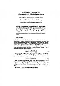
distribution, t distribution, and QA method CIs (SDs ⫽ .012, .009, and .008, respectively). In our simulations, we manipulated the heterogeneity variance, ␶2, with values 0, 0.04, 0.08, 0.16, and 0.32. One of the main problems of the z distribution CI is that its coverage probability decreases under the nominal level as the heterogeneity variance increases. Figure 1 shows the empirical coverage probabilities of the 36 CI procedures as a function of ␶2 for ␮ ⫽ 0.5, and Table 5 presents the empirical coverage probabilities for the two most extreme ␶2 values tested here: 0 and 0.32. As expected from previous studies, Figure 1A shows how the empirical coverage probability for CIs calculated assuming a normal distribution and estimated weights systematically decreased as ␶2 increased, regardless of the heterogeneity variance estimator used in calculating the weights. As Table 5 shows, the mean coverage probability through the eight ␶2 estimators for ␶2 ⫽ 0.32 was .920. Only when ␶2 ⫽ 0 did this CI procedure yield good coverage for all of the ␶2 estimators (mean estimated coverage ⫽ .963), with the exception of the HM and SJ estimators, which overstated the nominal confidence level (Ms ⫽ .977 and .984, respectively). The overstatement of the nominal confidence level obtained with the HM and SJ estimators was due to the fact that both of them are nonnegative estimators of ␶2 and, as a consequence, when ␶2 ⫽ 0, they are positively biased, leading to CIs that are too wide. For ␶2 ⱖ 0.04 and with the exception of the SJ estimator, the coverage probabilities for this CI procedure were inadmissibly under .94. Therefore, as ␶2 increases, the width of the CIs for the z distribution method becomes too narrow, with the consequence that the actual coverage is under the nominal level. The t distribution CI yielded coverage probabilities that also decreased as ␶2 increased for all the heterogeneity variance estimators (Figure 1B and Table 5). In contrast to the z distribution CI, however, as ␶2 increased, the actual coverage probability got closer to the nominal level. The unadjustment of the empirical coverage to the nominal level was more pronounced for small ␶2 values. Thus, for ␶2 ⫽ 0, the t distribution CI obtained coverage probabilities inadmissibly larger than the nominal level (mean estimated coverage through the eight ␶2 estimators ⫽ .977). For ␶2 ⫽ 0.32, the t distribution CI showed good coverage (mean estimated coverage probability ⫽ .947). Therefore, assuming a t distribution and the usual formula for the sampling variance seems to offer good coverage for large ␶2 values. The results found for the QA method were very similar to those of the t distribution CI: a better adjustment of the empirical coverage to the nominal level as ␶2 increased (Figure 1C and Table 5). In particular, for ␶2 ⫽ 0.32, the QA method achieved very good coverage (mean empirical coverage through the eight ␶2 estimators ⫽ .950), even slightly better than that of the t distribution CI. For ␶2 ⫽ 0, the mean coverage was clearly over the nominal level (mean esti-

1.000 OPTIMAL HS HE DL MBH HM SJ ML REML

0.975 0.950 0.925 0.900 0.0


D Empirical coverage probability

42


0.975 0.950 0.925 0.900 0.0


Figure 1. Average empirical coverage probabilities as a function of the ␶2 parameter, for the four confidence interval (CI) procedures with the eight heterogeneity variance estimators and the optimal weights (␮ ⫽ 0.5). A: z distribution CI. B: t distribution CI. C: quantile approximation method. D: weighted variance CI. HS ⫽ Hunter and Schmidt estimator; HE ⫽ Hedges estimator; DL ⫽ DerSimonian and Laird estimator; MBH ⫽ Malzahn, Bo¨hning, and Holling estimator; HM ⫽ Hartung and Makambi estimator; SJ ⫽ Sidik and Jonkman estimator; ML ⫽ maximum likelihood estimator; REML ⫽ restricted maximum likelihood estimator.


43

Table 5 Average Empirical Coverage Probabilities With Standard Deviations Through the 100 Simulated Conditions for Each Confidence Interval Procedure and Two Values of ␶2 (␮ ⫽ 0.5) Confidence interval procedure z distribution Weights

M

SD

t distribution M

SD

Weighted variance

QA method

M

SD

M

SD

.948

.002

.967

␶ ⫽0 .016

.950

.002

.970

.017

.956 .960 .958 .960 .977 .984 .955 .957

.006 .006 .007 .007 .003 .004 .006 .007

.972 .975 .973 .974 .986 .992 .971 .972

.017 .016 .017 .016 .008 .005 .017 .017

.948 .949 .948 .949 .952 .954 .948 .948

.006 .005 .006 .005 .004 .005 .006 .006

.974 .977 .975 .976 .988 .993 .974 .975

.017 .016 .018 .017 .008 .005 .018 .018

.950

.002

.972

.016

.947 .948 .947 .948 .948 .949 .946 .947

.007 .006 .006 .006 .004 .003 .008 .006

.942 .954 .950 .954 .946 .962 .944 .952

.005 .005 .007 .005 .012 .008 .007 .006

2

Optimal ␶2 estimator HS HE DL MBH HM SJ ML REML Optimal ␶2 estimator HS HE DL MBH HM SJ ML REML

.950

.002

.969

␶2 ⫽ 0.32 .016

.907 .926 .920 .926 .914 .936 .910 .922

.034 .026 .022 .023 .018 .021 .036 .023

.938 .951 .946 .951 .942 .959 .940 .948

.004 .003 .005 .004 .012 .008 .006 .005


mated coverage ⫽ .979) and slightly worse than that of the t distribution CI. The results for the QA method are similar to those found by Brockwell and Gordon (2007). The similarity of the results found for the t distribution and the QA method CIs is due to the fact that they only differ in the critical value used to calculate the CI: a critical value from a Student t distribution with k – 1 degrees of freedom and a quantile estimated from Equation 14 that is a function of k, respectively. For example, for k ⫽ 10, the respective critical values are 2.262 and 2.374. As both procedures propose the same sampling variance for the overall effect size, the width of the corresponding CIs is very similar and, as a consequence, the estimated coverage probabilities are also very close to each other. In any case, as ␶2 increases, the QA method seems to offer slightly better coverage than that of the t distribution CI. Whereas the z distribution, t distribution, and QA method CIs exhibited empirical coverages that were affected by the value of ␶2, the weighted variance CI achieved good coverage regardless of the value of ␶2 and the ␶2 estimator (Figure 1D), although always with a coverage probability slightly under the nominal confidence level. Even for ␶2 ⫽

0, the weighted variance CI outperformed the z distribution, t distribution, and QA method CIs. In fact, as Table 5 shows, for ␶2 ⫽ 0, the mean estimated coverage probability of weighted variance CIs through the eight ␶2 estimators was .949, whereas those of z distribution, t distribution, and QA method CIs were .963, .977, and .979, respectively. As a consequence, the weighted variance CI may be applied even for small values of ␶2. For ␶2 ⫽ 0.32, the mean empirical coverage for the weighted variance CI was .947, similar to that of the t distribution CI and slightly under that of the QA method. As Table 5 shows, the observed coverage probability with the weighted variance CI was less variable for each ␶2 estimator and through the eight ␶2 estimators than were those of the other three CI procedures. It seems that the improved formula for estimating the sampling variance proposed by Hartung (1999), together with the use of critical values from a Student t distribution, enables one to appropriately accommodate the uncertainty due to estimating the between-studies and within-study variances. With the optimal weights, the coverage probability of the four CI procedures was not affected by the value of ␶2 but,




0.975 0.950 0.925 0.900 0

20

40 60 80 Number of studies

100

120



0.975 0.950 0.925 0.900 0

20


100

120

C Empirical coverage probability

whereas z distribution and weighted variance CIs showed good coverage, the t distribution and the QA method CI overstated the nominal confidence level. This was an expected result, as to assume a t distribution for ␮ˆ or to simulate the empirical distribution of ␮ˆ when the optimal weights are known does not have a theoretical justification. Figure 2 shows the empirical coverage probabilities as a function of the number of studies in the meta-analysis (ks ⫽ 5, 10, 20, 40, and 100) for the 36 CIs. For small ks (5 and 10), the z distribution, t distribution, and QA method CIs showed a clear unadjustment of the empirical coverage probability to the nominal confidence level but, whereas the z distribution– based procedure showed empirical coverage probabilities under the nominal level, the t distribution and the QA method CIs presented coverage over the nominal level (see Figures 2A, 2B, and 2C). However, the weighted variance CI was able to maintain good coverage through the different values of k, regardless of the ␶2 estimator used (Figure 2D). A more detailed analysis enables us to distinguish the different performances of the four CI procedures. For k ⫽ 40 studies, ␮ ⫽ 0.5; ␶2 ⫽ 0.32; and, using the DL estimator of ␶2, the empirical coverage probabilities of the z distribution, t distribution, weighted variance, and QA method CIs were .935, .942, .949, and .945, respectively. With the REML ␶2 estimator, the observed probabilities were .939, .946, .949, and .949, respectively. That is, the weighted variance CI and the QA method showed the best adjustment to the nominal confidence level. Therefore, the QA method had a good performance for k ⫽ 40, in spite of the fact that the equation proposed by Brockwell and Gordon (2007) to estimate the critical values was obtained assuming k values not larger than 30. For k ⫽ 100 studies, ␮ ⫽ 0.5; ␶2 ⫽ 0.32; and, using the DL estimator of ␶2, the empirical coverage probabilities of the z distribution, t distribution, weighted variance, and QA method CIs were slightly lower than they were for k ⫽ 40, with the exception of the z distribution CI: .938, .940, .946, and .940, respectively. The same trend was found with the REML ␶2 estimator: .941, .944, .946, and .944 for the empirical coverage probabilities of the z distribution, t distribution, weighted variance, and QA method CIs, respectively. Thus, the performance of the QA method for k values larger than 30 was reasonably good, in spite of using k values over 30. In general, as k increased, the weighted variance CI performed better than the other three CI procedures. Finally, as Figure 3 shows, the average sample size of the meta-analyzed studies (Ns ⫽ 30, 50, 80, and 100) scarcely affected the performance of the CI procedures. As expected from the statistical theory, the CIs obtained with the optimal weights maintained good coverage through both the number of studies and the average sample size, regardless of the ␶2 estimator.


0.975 0.950 0.925 0.900 0

20


100

120

D Empirical coverage probability

44


0.975 0.950 0.925 0.900

0

20


100

120

Figure 2. Average empirical coverage probabilities as a function of the number of studies, k, for the four confidence interval (CI) procedures with the eight heterogeneity variance estimators and the optimal weights (␮ ⫽ 0.5). A: z distribution CI. B: t distribution CI. C: quantile approximation method. D: weighted variance CI. HS ⫽ Hunter and Schmidt estimator; HE ⫽ Hedges estimator; DL ⫽ DerSimonian and Laird estimator; MBH ⫽ Malzahn, Bo¨hning, and Holling estimator; HM ⫽ Hartung and Makambi estimator; SJ ⫽ Sidik and Jonkman estimator; ML ⫽ maximum likelihood estimator; REML ⫽ restricted maximum likelihood estimator.


45

Conclusions Empirical coverage probability


0.975 0.950 0.925 0.900 20

30

40

50 60 70 80 Average sample size

90

100 110



0.975 0.950 0.925 0.900 20

30

40


90

100 110


C 1.000 OPTIMAL HS HE DL MBH HM SJ ML REML

0.975 0.950 0.925 0.900 20

30

40


90

100 110


D 1.000 OPTIMAL HS HE DL MBH HM SJ ML REML

0.975 0.950 0.925 0.900 20

30

40


90

100 110

Figure 3. Average empirical coverage probabilities as a function of the average sample size, N៮ , for the four confidence interval (CI) procedures with the eight heterogeneity variance estimators and the optimal weights (␮ ⫽ 0.5). A: z distribution CI. B: t distribution CI. C: quantile approximation method. D: Weighted variance CI. HS ⫽ Hunter and Schmidt estimator; HE ⫽ Hedges estimator; DL ⫽ DerSimonian and Laird estimator; MBH ⫽ Malzahn, Bo¨hning, and Holling estimator; HM ⫽ Hartung and Makambi estimator; SJ ⫽ Sidik and Jonkman estimator; ML ⫽ maximum likelihood estimator; REML ⫽ restricted maximum likelihood estimator.

In meta-analysis, one of the main objectives is to estimate the parametric effect size by calculating an average effect size from the selected studies, ␮ˆ . When the underlying statistical model is a random-effects model, the average effect size is calculated by weighting each effect estimate by its inverse variance, the variance being the sum of the heterogeneity variance and the within-study variance. As both variances have to be estimated, the optimal weights, wi, are unknown in practice and so are substituted by estimated weights, wˆ i , by estimating both types of variances. Then, with the estimated weights, an average effect size is obtained and a CI for ␮ˆ is calculated assuming that ␮ˆ follows a standard normal distribution and that its sampling variance is defined by the usual formula, Vˆ共␮ˆ 兲 ⫽ 1/ i wî . However, this CI does not take into account the variability of the estimated variances of each study and, as a consequence, the width of the CIs is too narrow, leading to empirical coverage probabilities that are under the nominal confidence level unless the heterogeneity variance is null or very small. In spite of this problem, this CI procedure is the one applied most often in real meta-analyses. Our purpose in this article was to compare the performance of three alternative CI procedures with that of the standard one, in terms of the observed coverage probability. All of them are simple to calculate, not requiring intensive computation. Two of the three alternative CI procedures are based on the t distribution, but they differ in the formula to estimate the sampling variance of ␮ˆ : The procedure called here t distribution CI applies the usual sampling variance, Vˆ (␮ˆ ), whereas the other one, the weighted variance CI, assumes a less-known formula to estimate a weighted sampling variance of ␮ˆ , Vˆ w(␮ˆ ), proposed by Hartung (1999). The third alternative procedure, the QA method, assumes the usual sampling variance, Vˆ (␮ˆ ), but it proposes the estimation of the critical values for the CI, b1⫺␣/2, via Monte Carlo simulation of the quantiles of the M statistic (Brockwell & Gordon, 2007). Additionally, we examined the robustness of the four CI procedures to changes in the heterogeneity variance estimator, ␶2, as well as the influence of the value of ␶2; the number of studies, k; and the average sample size on the actual coverage probabilities of the CIs. With respect to the standard CI procedure (z distribution CI), our results coincided with those of previous simulation studies, showing coverage probabilities clearly under the nominal confidence level, unless ␶2 ⫽ 0 (Brockwell & Gordon, 2001, 2007; Follmann & Proschan, 1999; Hartung & Makambi, 2003; Makambi, 2004; Sidik & Jonkman, 2002, 2003, 2005, 2006; Viechtbauer, 2005). The performance of the standard procedure improved as the number of studies in the meta-analysis and the average sample size increased. The t distribution CI showed coverage probabilities over the nominal confidence level, in particular when

冘

46


the value of ␶2 and the number of studies were small. The failure of the z and t distribution CIs with the usual variance for ␮ˆ to achieve a good adjustment to the nominal confidence level is due to the fact that estimated values of ␶2 and ␴ 2i are used in place of the true values in the weights, implying that ␮ˆ follows neither an exact normal nor a t distribution. Moreover, both CI procedures present coverage probabilities that clearly depend on the heterogeneity variance estimator used in the computation of the weights, as well as on the value of ␶2 and the number of studies in the meta-analysis. Therefore, applying the usual sampling variance for ␮ˆ , Vˆ (␮ˆ ), with the estimated weights leads to CIs with empirical coverage probabilities that are not close to the nominal confidence level. Our results showed that the QA method and the weighted variance CI present good coverage, in general. The weighted variance CI, however, was more robust to changes in the ␶2 estimator than was the QA method. Thus, using eight different ␶2 estimators in our simulations enabled us to confirm the robustness of the weighted variance CI to changes in the ␶2 estimator and to extend the findings obtained in previous studies that only used two or three ␶2 estimators (Hartung & Makambi, 2003; Makambi, 2004; Sidik & Jonkman, 2003). Moreover, and in contrast to the QA method, the weighted variance CI yielded CIs that were affected neither by the value of ␶2 nor by the number of studies, k. Through all of the simulated conditions, this CI procedure achieved a good adjustment to the nominal confidence level and, in general, outperformed the z distribution, t distribution, and QA method CIs. If we consider that a good CI procedure to estimate the overall effect size in a meta-analysis, when the statistical model assumed is a random-effects model, should exhibit a good adjustment to the nominal confidence level regardless of the value of ␶2, the number of studies, the average sample size, and the heterogeneity estimator, then the weighted variance CI is clearly a better option than the usual CI procedure based on the normal distribution and than the t distribution CI. The results of our simulations coincide with those of previous Monte Carlo studies in showing a better performance of the weighted variance CI than of the z and t distribution CIs. With respect to the performances of the weighted variance CI and the QA method, our simulation study is the first one that compares these with each other. Our results show that although both of them exhibit, in general, good coverage in most of the conditions considered here, the weighted variance CI is less dependent on the value of ␶2, the number of studies in the meta-analysis, and the ␶2 estimator. In particular, the QA method offers deficient coverage when the heterogeneity variance and the number of studies are small, and it is more affected by the ␶2 estimator used to estimate the weights than is the weighted variance CI. Therefore, we recommend the use of the weighted variance CI in future meta-analyses.

Although we have focused on how to obtain a CI for the overall effect size, another advantage of assuming a t distribution for ␮ˆ with k – 1 degrees of freedom and the weighted sampling variance, Vˆ w(␮ˆ ), is that it is possible to test the null hypothesis of a parametric effect size equal to zero (H0: ␮ ⫽ 0) with the test statistic T ⫽ ␮ˆ / 冑Vˆw共␮ˆ 兲. Previous simulations have shown a better adjustment of this test statistic to the nominal significance level than that of the usual z statistic, based on the standard normal distribution and the usual sampling variance of ␮ˆ , z ⫽ ␮ˆ / 冑Vˆ共␮ˆ 兲 (Hartung, 1999; Hartung & Makambi, 2003; Makambi, 2004). Our study has some limitations. On the one hand, note that the results of our study can only be generalized to the simulated conditions in terms of ␶2 values, number of studies, and average sample sizes. On the other hand, we have examined the performance of the different CI procedures only for the standardized mean difference as the effect-size index. It is expected that the performance of the weighted variance CI obtained with the d index will be similar to that of meta-analyses that use other effect-size indices, provided they are relatively unbiased and follow an approximately normal distribution. In fact, previous simulation studies have found good performance of the weighted variance CI with such effect-size indices as the log odds ratio (Makambi, 2004; Sidik & Jonkman, 2002, 2006), the unstandardized mean difference (Hartung & Makambi, 2003), and the risk difference (Hartung & Makambi, 2003). Therefore, the good performance of the weighted variance CI seems to be robust to changes in the effect-size index. Finally, it is necessary to make some comments about the way we have applied the QA method. First, Brockwell and Gordon (2007) applied the QA method to the log odds ratio as the effect-size index, whereas we used the standardized mean difference. As Brockwell and Gordon (2007) stated, “the method is developed primarily for meta-analyses in which the effect of intervention is measured as a log odds ratio” (p. 4533). Changing the effect-size index can affect the performance of Brockwell and Gordon’s equation in estimating the critical values that are used in the QA method. However, as Brockwell and Gordon (2007) suggested, their equation for estimating the critical values could be applied provided the effect-size index is approximately normally distributed: While it is not firmly established that the QA method is suitable for meta-analyses on other scales, the development here relies on a structure which is not specific to log odds ratios, since the essence is estimators that are approximately normally distributed. (p. 4542)

Therefore, using their equation to estimate the critical values with standardized mean differences can be considered a sound practice. Second, in our simulation study, we used the equation proposed by Brockwell and Gordon (2007) to estimate the


quantiles of the M statistic (our Equation 14). They obtained the quantiles for M by means of a Monte Carlo simulation in which they varied the number of studies, k, between 2 and 30, and the heterogeneity variance, ␶2, between 0 and 0.5. In our simulation study, the number of studies ranged from 5 to 100, and the heterogeneity variance ranged from 0 to 0.32. Although our ␶2 values are in the range of those used by Brockwell and Gordon, we have applied their equation to meta-analyses with more than 30 studies, and this circumstance may produce suboptimal results for the QA method. It is not clear if using the equation proposed by Brockwell and Gordon (2007) for estimating the critical values is appropriate when the number of studies in a meta-analysis is larger than 30. Brockwell and Gordon (2007) considered that the range of k that they used “is likely to include the scope of almost all meta-analyses” (p. 4537), but they were referring to the medical literature. In psychology, metaanalyses have more than 30 studies relatively frequently and, as a consequence, this is not a trivial issue. If Brockwell and Gordon’s (2007) equation for calculating the critical values is only appropriate for the range of k values considered in their simulations, then the QA method loses generalizability. An alternative solution might be to find the equation to estimate the critical values by carrying out a Monte Carlo simulation to obtain the quantiles of the M statistic fixing the values of k (e.g., between 5 and 100) and ␶2 to be appropriate in a given research field. But in this case, the QA method loses simplicity because prior to the calculation of the CI (with our Equation 13), it is necessary to develop a Monte Carlo simulation to estimate the critical values. Our results showed a reasonably good coverage of the QA method for k ⬎ 30, but more research is needed to determine the generalizability of the QA method for different ranges of k and effect-size indices.

References Aptech Systems. (2001). The GAUSS Program (Version 3.6) [Computer software]. Kent, WA: Author. Biggerstaff, B. J., & Tweedie, R. L. (1997). Incorporating variability estimates of heterogeneity in the random effects model in meta-analysis. Statistics in Medicine, 16, 753–768. Brockwell, S. E., & Gordon, I. R. (2001). A comparison of statistical methods for meta-analysis. Statistics in Medicine, 20, 825– 840. Brockwell, S. E., & Gordon, I. R. (2007). A simple method for inference on an overall effect in meta-analysis. Statistics in Medicine, 26, 4531– 4543. Cohen, J. (1988). Statistical power analysis for the behavioral sciences (2nd ed.). Hillsdale, NJ: Erlbaum. Cooper, H. M. (1998). Integrating research: A guide for literature reviews (2nd ed.). Thousand Oaks, CA: Sage. DerSimonian, R., & Laird, N. (1986). Meta-analysis of clinical trials. Controlled Clinical Trials, 7, 177–188.

47

Egger, M., Smith, G. D., & Altman, D. G. (Eds.). (2001). Systematic reviews in health care: Meta-analysis in context (2nd ed.). London: British Medical Journal. Field, A. P. (2001). Meta-analysis of correlation coefficients: A Monte Carlo comparison of fixed- and random-effects methods. Psychological Methods, 6, 161–180. Field, A. P. (2003). The problems of using fixed-effects models of meta-analysis on real-world data. Understanding Statistics, 2, 77–96. Fleiss, J. L. (1994). Measures of effect size for categorical data. In H. Cooper & L. V. Hedges (Eds.), The handbook of research synthesis (pp. 245–260). New York: Russell Sage Foundation. Follmann, D. A., & Proschan, M. A. (1999). Valid inference in random effects meta-analysis. Biometrics, 55, 732–737. Grissom, R. J., & Kim, J. J. (2005). Effect sizes for research: A broad practical approach. Mahwah, NJ: Erlbaum. Haddock, C. K., Rindskopf, D., & Shadish, W. R. (1998). Using odds ratios as effect sizes for meta-analysis of dichotomous data: A primer on methods and issues. Psychological Methods, 3, 339 –353. Hardy, R. J., & Thompson, S. G. (1996). A likelihood approach to meta-analysis with random effects. Statistics in Medicine, 15, 619 – 629. Hartung, J. (1999). An alternative method for meta-analysis. Biometrical Journal, 41, 901–916. Hartung, J., & Makambi, K. H. (2002). Positive estimation of the between-study variance in meta-analysis. South African Statistical Journal, 36, 55–76. Hartung, J., & Makambi, K. H. (2003). Reducing the number of unjustified significant results in meta-analysis. Communications in Statistics: Simulation and Computation, 32, 1179 –1190. Hedges, L. V. (1983). A random effects model for effect sizes. Psychological Bulletin, 93, 388 –395. Hedges, L. V., & Olkin, I. (1985). Statistical methods for metaanalysis. Orlando, FL: Academic Press. Hedges, L. V., & Vevea, J. L. (1998). Fixed- and random-effects models in meta-analysis. Psychological Methods, 3, 486 –504. Hunter, J. E., & Schmidt, F. L. (1990). Methods of meta-analysis: Correcting error and bias in research synthesis. Beverly Hills, CA: Sage. Hunter, J. E., & Schmidt, F. L. (2004). Methods of meta-analysis: Correcting error and bias in research synthesis (2nd ed.). Newbury Park, CA: Sage. Lipsey, M. W., & Wilson, D. B. (2001). Practical meta-analysis. Thousand Oaks, CA: Sage. Makambi, K. H. (2004). The effect of the heterogeneity variance estimator on some tests of treatment efficacy. Journal of Biopharmaceutical Statistics, 14, 439 – 449. Malzahn, U. (2003). Meta-analysis: A general principle for estimating heterogeneity variance in several models. In R. Schulze, H. Holling, & D. Bo¨hning (Eds.), Meta-analysis: New developments and applications in medical and social sciences (pp. 41–52). Cambridge, MA: Hogrefe & Huber. Malzahn, U., Bo¨hning, D., & Holling, H. (2000). Nonparametric

48


estimators of heterogeneity variance for standardised difference used in meta-analysis. Biometrika, 87, 619 – 632. Overton, R. C. (1998). A comparison of fixed-effects and mixed (random-effects) models for meta-analysis tests of moderator variable effects. Psychological Methods, 3, 354 –379. Raudenbush, S. W. (1994). Random effects models. In H. Cooper & L. V. Hedges (Eds.), The handbook of research synthesis (pp. 301–321). New York: Russell Sage Foundation. Raudenbush, S. W., & Bryk, A. S. (1985). Empirical Bayes metaanalysis. Journal of Educational Statistics, 10, 75–98. Rosenthal, R. (1991). Meta-analytic procedures for social research (Rev. ed.). Newbury Park, CA: Sage. Rosenthal, R. (1994). Parametric measures of effect size. In H. Cooper & L. V. Hedges (Eds.), The handbook of research synthesis (pp. 231–244). New York: Russell Sage Foundation. Rosenthal, R., Rosnow, R. L., & Rubin, D. B. (2000). Contrasts and effect sizes in behavioral research: A correlational approach. Cambridge, UK: Cambridge University Press. Sańchez-Meca, J., & Marıń-Martıńez, F. (1998). Testing continuous moderators in meta-analysis: A comparison of procedures. British Journal of Mathematical and Statistical Psychology, 51, 311–326. Sańchez-Meca, J., Marıń-Martıńez, F., & Chacoń-Moscoso, S. (2003). Effect-size indices for dichotomized outcomes in metaanalysis. Psychological Methods, 8, 448 – 467. Shadish, W. R., & Haddock, C. K. (1994). Combining estimates of effect size. In H. Cooper & L. V. Hedges (Eds.), The handbook

of research synthesis (pp. 261–281). New York: Russell Sage Foundation. Sidik, K., & Jonkman, J. N. (2002). A simple confidence interval for meta-analysis. Statistics in Medicine, 21, 3153–3159. Sidik, K., & Jonkman, J. N. (2003). On constructing confidence intervals for a standardized mean difference in meta-analysis. Communications in Statistics: Simulation and Computation, 32, 1191–1203. Sidik, K., & Jonkman, J. N. (2005). Simple heterogeneity variance estimation for meta-analysis. Journal of the Royal Statistical Society, Series C: Applied Statistics, 54, 367–384. Sidik, K., & Jonkman, J. N. (2006). Robust variance estimation for random effects meta-analysis. Computational Statistics and Data Analysis, 50, 3681–3701. Sidik, K., & Jonkman, J. N. (2007). A comparison of heterogeneity variance estimators in combining results of studies. Statistics in Medicine, 26, 1964 –1981. Viechtbauer, W. (2005). Bias and efficiency of meta-analytic variance estimators in the random-effects model. Journal of Educational and Behavioral Statistics, 30, 261–293. Viechtbauer, W. (2007). Confidence intervals for the amount of heterogeneity in meta-analysis. Statistics in Medicine, 26, 37– 52.

Received March 29, 2007 Revision received October 24, 2007 Accepted December 20, 2007 䡲

E-Mail Notification of Your Latest Issue Online! Would you like to know when the next issue of your favorite APA journal will be available online? This service is now available to you. Sign up at http://notify.apa.org/ and you will be notified by e-mail when issues of interest to you become available!

Confidence Intervals for the Overall Effect Size in ... - Semantic Scholar

Confidence Intervals for the Overall Effect Size in ... - Semantic Scholar

Suggest Documents

Confidence Intervals for the Overall Effect Size in Random ... - CiteSeerX

Confidence Intervals For An Effect Size When ... - Semantic Scholar

eAppendix Confidence Intervals Confidence intervals for the ...

Understanding confidence intervals - Semantic Scholar

Confidence Intervals for Computational Effort ... - Semantic Scholar

Nonparametric confidence intervals for monotone ... - Semantic Scholar

Binomial Distribution Sample Confidence Intervals ... - Semantic Scholar

Confidence Intervals for the True Classification ... - Semantic Scholar

Simultaneous Confidence Intervals and Sample Size Determination ...

generalized confidence intervals for the largest ... - Semantic Scholar

simultaneous confidence intervals for

Confidence intervals

Confidence Intervals Our Goal in Inference Confidence Intervals (CI)

CONFIDENCE INTERVALS VS BAYESIAN INTERVALS

Rapid Approximation of Confidence Intervals for ... - Semantic Scholar

Bootstrap Confidence Intervals for Ratios of ... - Semantic Scholar

Confidence intervals for half-life deviations from ... - Semantic Scholar

Confidence intervals for pulsed mass extinction ... - Semantic Scholar

Confidence Intervals for OD Demand Estimation - Semantic Scholar

Confidence regions and intervals in nonlinear ... - Semantic Scholar

Confidence Trick: The Interpretation of Confidence Intervals

Confidence intervals for correlations - Stata

Confidence Intervals for One Mean

Calculating the Confidence Intervals Using Bootstrap - Semantic Scholar