International Econometric Review (IER)
Confirmation, Correction and Improvement for Outlier Validation using Dummy Variables Arzdar Kiraci Siirt University ABSTRACT Dummy variables can be used to detect, validate and measure the impact of outliers in data. This paper uses a model to evaluate the effectiveness of dummy variables in detecting outliers. While generally confirming some findings in the literature, the model refutes the presumption that the t˗statistic or the F˗incremental statistic is enough to validate an observation as an outlier. In order to rectify this fallacy, this paper recommends an easily-calculable robust standardized residual statistic that is more compatible with the definition of outliers. The robust standardized residual statistic suggested herein is still used in many robust regression methods and is more effective than the t˗statistic or the F˗incremental statistic in validating outliers with dummy variables. The results of this study suggest some practical recommendations for dealing with outliers and improvements in maintaining the integrity of data. We recommend all previous studies using this statistics be revised in light of the findings presented in this paper. Key.words: Dummy Variable, t˗Statistic, Outlier, Robust Dummy Statistic, Robust Standardized Residual JEL Classifications: C2, C20, C51, C52 AMS 2000 subject classifications: Primary 60K35, 60K35; secondary 60K35
1. INTRODUCTION Outliers are defined as observations that do not obey the (linear) pattern formed by the majority of the observations, and if they are influential they give rise to misleading results (Rousseeuw and Van Aelst, 1999). During regression analysis, a dummy variable (DV) or indicator variable is introduced for an observation that is suspected to be affected by different variables other than the ones in the model. In some cases these suspicious observations may turn out to be significant outliers. The standard in the literature has been to assign a DV to each outlier observation, which is then validated as an outlier using the t-statistic of the DV. If a search is performed in academic journal databases (for example, in Business Source Complete) thousands of studies are found in 2010 that identify outliers using the t˗statistic of the DV. This paper investigates the following questions: If there are many reasons for outliers like an economic shock, a technological breakthrough, a natural disaster, even an incorrect recording of observation, or, alternatively stated, if an outlying observation is created under the influence of a rare occurring and unpredictable incident (variable) then can a DV represent
Arzdar Kiraci, Siirt University, Faculty of Economics and Administrative Sciences, Gures Caddesi 56100 Siirt/Turkey, (email:
[email protected],
[email protected]), Tel: +90 (484) 223 12 24 - 223 17 39 224 11 38, Fax: +90 (484) 223 19 98.
43
Kiraci-Confirmation, Correction and Improvement for Outlier Validation using Dummy Variables
this event? If a DV is used for each outlier, then how are the statistics in Ordinary Least Squares (OLS) affected? Is the t˗statistic of DVs or the F˗incremental statistic successful in identifying these outliers? Is there a statistic that is easier to calculate? This paper answers these questions. As noted by Greene (2002:117), if a DV is used for an observation it has the effect of deleting that observation from the computation of OLS parameters and standard error (SE). Studenmund (2002:224) has, in accordance, advanced evidence that the dummy variable coefficient is equal to the studentized residual for that observation, which is also proven in the following section. This is an advantage because many robust regression techniques identify outliers by deleting suspicious observations from the data according to a selected criterion. One important point that is not emphasized in the literature is that the ratio of the dummy coefficient to the SE of the regression is the robust standardized residual (RSR). RSR is also referred to as the deleted studentized residual, externally studentized residual or jackknifed residual (Rousseeuw and Leroy, 1987:226), which is still used in many robust regression methods. However, the t˗statistic, which will be shown to be unsuccessful, is still widely used in the literature. As an alternative to the t˗statistic this paper recommends the use of the dummy coefficient to SE ratio as a new robust RSR statistic. This statistic is easier to calculate than Cook's distance (which measures the change in the estimates that result from deleting each observation, Cook, 1985), DFFITS (which is the predicted value for a point, obtained when that point is left out of the regression, Billingsley et.al., 1980) or DFBETAS (which is the scaled measure of the change in each parameter estimate and is calculated by deleting the ith observation, Billingsley et.al., 1980). The next section explains the notation and the model used in this paper to derive an important statistic based on DVs. The third section introduces this new statistic, and the fourth section presents an example, through which the insufficiency of the t˗statistic of the DV or the F˗incremental statistic is illustrated. Finally, the conclusion part summarizes the findings of this paper with suggestions for future research. 2. THE MODEL For the given data let there be n observations with v.+.1 independent variables and n.– m suspicious observations be represented by n.– m different DVs. Let Y'.=.[y1.....ym]1×m be the dependent variable vector for the observations without DVs, Y'd.=.[ym+1......yn]1×(n–m) be the dependent variable vector for the observations with DVs, xi.=.[1.xi,1.....xi,v]1×(v+1) be the independent variable vector for ith observation, X'.=.[x'1.....x'm](v+1)×m be the independent variable matrix for the observations without DVs, and X'd.=.[x'm+1.....x'n](v+1)×(n–m) be the independent variable matrix for the observations with DVs. Let 0m×(n–m) be the zero matrix, εm×1 be the error vector, εd be the (n.–.m)×1 error vector that contains the outlier information, and I(n–m)×(n–m) be the unit matrix. Then the regression model can be written as follows: Y X 0 β ε (2.1) Y X I δ ε d d d Proposition 2.1. The OLS estimator for β(v+1)×1 and δ(n–m)×1 is given by: b (X' X)-1 X' Y d Yd - X d b 44
(2.2)
International Econometric Review (IER)
The residuals and other important statistics can be calculated as follows: e Y X 0 b Y - Xb e Y X d d d I d 0
(2.3)
In equation (2.2) b is the OLS estimator of X, i.e.; it is not affected by the suspicious observations represented by DVs. Therefore, the DVs have the effect of omitting these observations from the computation of OLS parameters (Greeen, 2002:117). If residual values for the dummy variables are required, they can be calculated as Yd.–.Xdb.=.d, namely as the coefficients of DVs in (2.2), but not as the 0 vector in (2.3) (Studenmund, 2002:224). Hence, the DV coefficients are successful in representing the information contained in suspicious observations, and their coefficient values are a measure of their influence on the OLS regression results. The DVs have the same effect of deleting these observations from the computations of the SE ( ) and cov(b). These estimators can be calculated as follows: e e ed e d ee (Y - Xb)(Y - Xb) var ˆ 2 n (v n m 1) m v 1 m v 1 -1 -1 (XX) - (XX) Xd b cov( ) ˆ 2 -1 -1 d - X d (XX) (I X d (XX) Xd ) For the coefficient of determination R2, adding a DV does not have the same effect of deleting the suspected observations from the computation as proven in the following proposition. Proposition 2.2. Let R2 be the coefficient of determination in a regression with DVs and R20 be in a regression without any suspicious observations. Then, R2.>.R20.1 3. PROPOSAL OF AN ALTERNATIVE ROBUST DUMMY STATISTIC TO THE T˗STATISTIC OR F˗INCREMENTAL STATISTIC In the literature on robustness, an observation can be identified as an outlier by the robust standardized residual (RSR) value, which is the ratio of the residual value of that observation to the SE of the regression. Both the residual value and the SE are calculated using robust estimators that are not affected by any outliers. As mentioned previously, for a regression with DVs, the ratio of the dummy coefficient to SE of the regression gives the RSR for that observation. Alternatively, for observation j this value can be written as follows: d RSR j j (3.4) ˆ This RSR j is the robust dummy statistic suggested by this paper. For an outlier observation this RSRj of a DV is compared with the tj value of a DV in the following proposition. Proposition 3.3. The t˗statistic of a DV is unable to validate outliers with large X independent variable values.
1
While equality is possible, it would not make the observations suspicious.
45
Kiraci-Confirmation, Correction and Improvement for Outlier Validation using Dummy Variables
According to the proof of proposition 3.3, provided in the Appendix, it is impossible to assign critical values to the calculated t˗values of DVs, because they will depend on Xd or outliers. The same conclusion can be stated for the F˗incremental statistic as shown in the following proposition. Proposition 3.4. The F˗incremental statistic is unable to validate outliers with the average of Yd dependent variable values of outliers close to the average of Y dependent variable values of other observations. In the following part, the problems that may arise as a result of using the t˗statistic or the F˗incremental statistic instead of the RSR value are illustrated with an example. 4. ILLUSTRATIVE EXAMPLE For the simple regression model yi.=.β0.+.β1.xi.+.εi (εi. .N(0,σ2)), using a software program written in Octave, different values for the parameters β0, β1,.σ2 are generated, and an outlier is placed. Figure 4.1 Plot for the data in Table 4.1. 2,0000
1,5000
1,0000
0,5000
y = 0,8244 + 0,0277x R² = 0,4205
0,0000 -60,0
-50,0
-40,0
-30,0
-20,0
-10,0
0,0
10,0
-0,5000 y = 1,0314+ 0,0529x R² = 0,3906 -1,0000 Obs.
y
x Obs.
y
x Obs.
y
x
1 2
1.368872 0.005 1.529872 -0.980
8 9
0.912649 -0.059299
-6.680 -7.595
15 16
0.317508 -12.875 0.802124 -13.720
3 4
0.514864 -1.955 1.256283 -2.920
10 11
0.452557 0.519466
-8.500 -9.395
17 18
-0.051358 -14.555 0.089404 -15.380
5 6
0.396734 -3.875 0.363789 -4.820
12 13
0.951551 -10.280 0.615652 -11.155
19 20
0.244413 -16.195 0.149377 -17.000
7
0.463096 -5.755
14
0.501619 -12.020
21
-0.422100 -55.450
Table 4.1 Data for the example.
46
International Econometric Review (IER)
The data in Table 4.1 is generated using yi.=.1.+.0.049307299.xi.+.εi.(εi. .N(0,0.32)). The last (21st) observation is an outlier as illustrated in Figure.4.1, where the OLS estimator deviates considerably from the linearity indicated by the majority of observations. Important statistics are presented in Table.4.2 along with the outlier, in Table .4.3 without the outlier, and in Table.4.4 where a DV is used for the outlier observation. For the regression results with the outlier included in the data in Table.4.2, all of the coefficients are statistically significant. In Table.4.2 the Durbin-Watson statistic is 1.93,thus there is no sign of autocorrelation or model specification error. However, the results are biased, because the data contains an outlier. The 99% confidence interval for the slope estimator in Table.4.2 is (0.006349, 0.048997), and it does not contain the true population parameter 0.049307, while the 99% confidence interval for the slope estimator in Table.4.3 is (0.008339, 0.097426). For the regression results without the outlier in the data in Table.4.3, again, all of the coefficients are statistically significant. The Durbin-Watson statistic is 2.17, hence there may not be an autocorrelation or model specification error. Coefficient
SE
t stat
p-value
Intercept
0.824398
0.116728
7.0625483
1.01E-06
Slope
0.027673
0.007454
3.7127689
1.47E-03
R2 Std. Error
0.420461 0.380587
Obs.
21
F
13.784653
DW d 1.9342573
Table 4.2 Regression results with the outlier. Coefficient
SE
t stat
p-value
Intercept
1.031396 0.1586173
6.5024186
4.09E-06
Slope
0.052882 0.0155696
3.3965079
3.22E-03
R2 Std. Error
0.390580 0.359492
Obs. F
20 11.5362659
DW d 2.1729233
Table 4.3 Regression results without the outlier. Coefficient
SE
t stat
p-value
Intercept
1.031396 0.1586173
6.5024185
4.09E-06
Slope Dummy
0.052882 0.0155696 1.478817 0.8146362
3.3965079 1.8153101
3.22E-03 0.086175
RSR
4.113634
R2
0.510141
Std. Error
0.359492
Obs. F
21 9.372650
Table 4.4 Regression results with a dummy variable for the outlier.
47
Kiraci-Confirmation, Correction and Improvement for Outlier Validation using Dummy Variables
Unfortunately, the OLS regression results are not immune to masking effect of outliers (Rousseeuw and Leroy, 1987). The situation does not change if a DV is added for the suspicious observation. If the outlier is represented with a DV, the t˗statistic of the DV is (1.82), and it is statistically insignificant at a 5% significance level. In addition, the F˗incremental statistic is 4.39 (Fcr.=.4.41 at a 5% significance level), which does not indicate the presence of an outlier. However, the RSR statistic, which is used to identify outliers in the literature on robust regression where an observation is identified as outlier if RSR.>.2.5 in value (Rousseeuw and Leroy, 1987), indicates an outlier with an RSR value of.4.11. As theoretically proven and as illustrated in Table .4.3 and Table.4.4, when a DV is used for an outlier, it has the effect of deleting that observation from the computation of the OLS parameters. Furthermore, adding a DV for an outlier increases the R2 value, while the F˗value may increase or decrease. Using a software program written in Octave, different data are generated, and one outlier is placed in each data. In some of data the t˗statistic of a DV or F˗incremental statistic failed to validate outliers that were highly influential, which in certain cases even caused the slope coefficients to change from positive significant to negative significant or vice versa. 4. COMMENTS AND CONCLUSION This paper proves that the t˗statistic of a DV or the F˗incremental statistic are not always effective in validating outliers; this argument is both theoretically proven and illustrated with an empirical example. Therefore, these statistics should not be used. Proposed in place of these statistics is an alternative statistic, which is consistent with the standards for outlier detection methods in the literature on robustness. If a DV is used for an outlier observation it has the effect of deleting that observation from computation of OLS parameters and standard error (Greene, 2002). However, if the dummy variable is used in the model, then the coefficient of determination, R2, always increases. In addition, according to proposition 3.3, it is impossible to assign critical values to the calculated t˗value of a DV, because they will depend on Xd or outliers. In the literature on robust regression the debate about whether to keep outliers in data or to remove them continues. According to the findings in this paper, instead of using outlier observations with DVs, removing the outlier (and its DV) might be more appropriate for scientific inference, because using DVs for outliers has the effect of deleting that observation from computation of OLS parameters and SE. However, as shown in the proof of proposition 2.2, included in the Appendix, using DVs for outliers always increases the R2 statistic. As mentioned in Studenmund (2002), the dummy's coefficient equals the residual for that observation. In the literature on robustness, RSR, which is used to detect outliers, is calculated by dividing the residual of the observation by the SE of the regression. This paper suggests that the ratio of the DVs coefficient to the SE of the regression be used as the method for outlier detection, because this ratio is the RSR of that observation. This RSR value, which is the robust dummy statistic suggested by this paper is easier to calculate than Cook's distance (Cook, 1985), DFFITS (Billingsley et.al., 1980), or DFBETAS (Billingsley et.al., 1980). In addition, RSR of a DV is a residual value that gives the magnitude of the information contained in the suspicious observations and their values are a measure of their influence on OLS results when they are included in the data without DVs. 48
International Econometric Review (IER)
The illustrative example provided in this paper proves that the t˗statistic of a DV or the F˗incremental statistics are not always successful in identifying outliers. This paper aims to provide scientists with a better alternative for outlier validation, namely the RSR statistic, derived from the techniques/ideas in robust regression methods. The findings of this paper both theoretically and empirically demonstrate the superiority of the RSR statistic to the t˗statistic and the F˗incremental statistic. If there is prior information that correctly identifies a group of observations in which all of the outliers are contained then using the findings of this paper the RSR statistic of DV will enable the accurate detection of all outliers. Using the RSR statistic of DV is not an advanced technique, and is in fact easier and faster to calculate than most other robust regression techniques. One important warning must be given about the use of DVs with outliers: due to the masking effect, the detection/validation of outliers using the RSR statistic of DVs works correctly only if all possible outliers are in the group of observations represented by DVs. If there is no prior information on which observations are outliers, all of the outliers have to first be identified using any of the other robust techniques for outlier detection, but these advanced techniques require a lot of computer calculation2. Only then can outliers be validated and their effects be analyzed or measured using the RSR statistic of DV. APPENDIX Proof of Proposition 2.1: Without loss of generality, the places of Y and Yd in equation (2.1) can be interchanged to make matrix inversion easier, thus the OLS estimator becomes: 1 d I X d I X d I X d Yd b 0 X 0 X 0 X Y d I b X d
1
Xd Yd XX Xd X d XY Xd Yd
From the property of inverses of partitioned matrices in Frees (2004:420) or Timm (2002:46) 1
I Xd (I X d ( XX)-1 Xd ) - X d ( XX)-1 X XX X X ( XX)-1 X ( XX)-1 d d d d Yd d (I X d ( XX)-1 Xd ) - X d ( XX)-1 b -1 -1 ( XX) ( XX) Xd X Y Xd Yd d Yd - X d (X' X)-1 X' Y b (X' X)-1 X' Y
QED.
2
Zaman et al. (2001) is a good example for the use and explanation of these advanced techniques.
49
(A.5)
Kiraci-Confirmation, Correction and Improvement for Outlier Validation using Dummy Variables
Proof of Proposition 2.2: Let R2 be the coefficient of determination in the regression with DV and R20 be the one without suspicious observations in data, which can be formulated as follows: e e ed ee e d 1 R2 1 n n ( yi y ) 2 ( yi y ) 2 i 1
R02 1
ee m
(y i 1
n
m
i 1
i 1
i
i 1
y0 ) 2
where y ( yi / n) and y0 ( yi / m) ; The relation between ӯ and ӯ0 is y y0 ( n
Then
m
( yi y ) 2 ( yi y0 ) i 1
2
i 1
m
m
i 1
i 1
n mn y 0 yi ) y 0 n i m 1 n
(y
i m 1
i
y)2 n
( yi y0 ) 2 2 ( yi y0 ) m 2 ( yi y ) 2 m
( yi y0 ) 2 m 2 i 1
i m 1
n
( y
i m 1
m
i
y ) 2 ( yi y 0 ) 2 i 1
n
m
i 1
i 1
( yi y ) 2 ( yi y 0 ) 2 This implies that the denominator of the negative term in R2 is larger than the one in R20. Hence R2.>.R20. QED. Proof of Proposition 3.3: For observation j the t˗statistic of DV can be represented as follows: dj RSR tj ˆ ( XX) jj1 ( XX) jj1 It should be noted that the t˗statistic contains a robust term (RSR) and a non-robust term, namely, ( XX ) jj1 . This can be shown as follows: From equation (A.5) terms for the dummies can be calculated with the suitable element in the diagonal of (I X d ( XX)-1 Xd ) . Let (XX)-1 be:
c11 c1( v1) (XX)-1 c( v1)1 c( v1)( v1) 1 then the diagonal of ( XX ) jj becomes: 50
International Econometric Review (IER) v
v
g 0
h 0
( XX) jj1 (I X d ( XX)-1 Xd )ii 1 xig c( h1)( g 1) xih . .
.
. .
.
. .
.
where i = (j–m), xab = x(a+m)b, a = 1... (n–m), b = 1... v, xa 0 =.1 if the regression with a constant is considered and xa 0 =.0 if the regression without a constant is considered. From this equation even one outlier in x direction, i.e. a large xab in one observation can make ( XX ) jj1 >>1, which is possible in situations where RSRj.>.2.5 and tj.