Connected Coverage in Wireless Networks with Directional Antennas

Connected Coverage in Wireless Networks with Directional Antennas ∗ Department

Zuoming Yu∗‡ , Jin Teng† , Xiaole Bai† , Dong Xuan† and Weijia Jia‡

of Mathematics, Jiangsu University of Science and Technology, China. [email protected] Science and Engineering, The Ohio State University, USA. {tengj, baixia, xuan}@cse.ohio-state.edu ‡ Department of Computer Science, City University of Hong Kong, Hong Kong SAR. [email protected]

† Computer

Abstract—In this paper, we address a new unexplored problem - what are the optimal patterns to achieve connected coverage in wireless networks with directional antennas. As their name implies, directional antennas can focus their transmission energy in a certain direction. This feature leads to lower cross-interference and larger communication distance. It has been shown that with proper scheduling mechanisms, directional antennas may substantially improve networking performance in wireless networks. In this paper, we propose a set of optimal patterns to achieve full coverage and global connectivity under two different antenna models, i.e., the sector model and the knob model. We also introduce with detailed analysis several fundamental theorems and conjectures. Finally, we examine a more realistic sensor model, where sensing range and communication range may both vary randomly. Results show that our designed patterns work well even in unstable and fickle physical environment.

I. I NTRODUCTION Directional antennas are able to promote communication quality by focusing transmission energy in one direction and reducing interference and fading. In the past several years there have been substantial breakthroughs in the miniaturization of directional antennas [9], [16], [18]. In the near future, we will see extensive applications of directional antennas in wireless networks. Echoing this trend, there has recently been great interest in using directional antennas on individual nodes to improve the general performance of wireless networks, especially wireless sensor networks (WSNs) [7], [8], [12], [17], [20], [21]. The problem of optimal node deployment in wireless networks with directional antennas is a significant emerging issue. In wireless networks, coverage guarantees satisfactory service provision, and connectivity means the networking infrastructure is connected for exchange of information. For example, the sensing service provided by WSNs should cover the entire region of interest, while all sensor nodes should be able to communicate with each other. In cellular networks, the base-stations are supposed to serve clients at any place in the service area, and there must be a connected channel for basestations to establish a circuit switch session or exchange data packets. Optimally deploying nodes to achieve full coverage and global connectivity in wireless networks has long remained a fundamental problem of both theoretical and engineering interest. Besides such immediate benefits of lower costs and better network management, optimal patterns can also serve

rs Ƚ௖

rc

(a)

(b)

rc

rs Ƚ௖ (c)

(d)

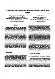
Fig. 1. The Optimal Patterns. Dotted circles with radius rs are the sensing range, solid shaded sectors with radius rc are the communication range and solid lines in (b)(d) are wireless connections. (a) and (b) show the wave patterns, which are optimal for nodes with large communication angles, i.e. αc ≥ π/3. Two adjacent line of nodes form a connected and full covering band. (c) and (d) show the line pattern, which is optimal for nodes with small communication angles. Every line of nodes forms a connected and full covering band. Connected bands in both the wave and line patterns are connected by nodes strewn on the sides.

to guide optimization in random deployments. Pioneering research in this field has established some theoretical guidelines [13], [24]. Several optimal patterns have also been proposed for certain types of wireless networks [1], [3], [4]. However, all these theories and patterns are based on the assumption of omnidirectional sensors and antennas. Essentially, optimal deployment that achieves both connectivity and full coverage in wireless networks with directional antennas is not addressed. In this paper, we will address this new problem, i.e. designing optimal patterns for connected coverage in wireless networks with directional antennas. In particular, this paper makes the following four contributions: 1. To the best of our knowledge, we are the first to study the antenna directivity in the connected coverage problem for optimal deployment pattern. In the process of designing optimal patterns for directional antennas, we also provide a new analysis methodology based on combinatorial geometry. The concept of tiling is introduced to help construct the largest

2

sensing Voronoi polygons. Our method of giving a lower bound on the covering density and “tapering” the Voronoi polygons to achieve this bound can be widely applied in optimality analysis of other connected coverage problems. 2. For the sector communication model of directional antennas, we design two typical optimal patterns, the wave pattern and the line pattern, as are shown in Fig. 1. The wave patterns include the Sharp Wave Pattern (SWP) and the Gentle Wave Pattern (GWP). The difference between them is the sharpness of the wave. The line pattern only has one variety, the Local Circulation Pattern (LCP). The SWP is applicable to most scenarios, when the antenna covering angle and range are both large. The SWP must be complemented by the GWP when the communication range is fairly small. However, when communication angles are critically limited, i.e., the main lobe beamwidth is less than π/3, the LCP has better performance in terms of node saving. And we surprisingly find that the optimal patterns do not change with αc within the region where the same type of wave or line pattern, i.e., SWP, GWP or LCP, remains optimal. 3. We also prove that our designed patterns are still optimal, when more rigorous communication models are adopted, e.g., the knob model, which is a larger sector plus a smaller circle at its base. From here, we gain insight into the connectivity that in order for wireless networks to become globally connected, enhanced radiation ability in one direction, i.e., the main lobe, is decisive, while the sidelobes only play a secondary role. 4. In order for our optimal patterns to be more robust in real applications, we address several practical issues. Realistic sensing and communication models are studied in detail. In real applications, sensors and antennas may exhibit unpredictable attenuation and fading. We evaluate the impact of all these factors on our proposed optimal patterns, and show that our designed patterns work well in realistic settings. The rest of the paper is organized as follows. We briefly compare our new directonal problem with the traditional omnidirectional problem in Section II. We formally introduce the problem and the communication models in Section III. In Section IV, we present, with proof, the optimal patterns under the sector and the knob communication model. We study in Section V the optimality of our designed patterns under more realistic sensing and communication models. Section VI introduces the related work, and Section VII concludes the whole paper. II. K EY D IFFERENCE WITH D IRECTIONAL A NTENNAS Deploying nodes with directional antennas is very different from deploying omnidirectional ones. More factors, such as communication angle, node orientation and link asymmetry, must be taken into consideration, as is illustrated in Fig. 2. And the actual optimal patterns for directional antennas, for which we will provide proof later in the paper, display some unique features which make them curiously different from their omnidirectional counterpart.

Fig. 2. In (a), node A and B can communicate with each other. However, in (b), A may connect to B, but not vice versa. In (c), node A and B point directly to each other establishing a bidirectional link. In (d), a circulation chain of connections enables A and B to communicate bidirectionally.

A. Special Challenges When it comes to designing optimal patterns for wireless networks with directional antennas, some distinctive difficulties immediately attract our notice. We must find solutions to these new challenges before we can claim any optimality of the designed patterns. We list these challenges as follow: 1) Node Orientation: For nodes with omnidirectional antennas, it does not matter how they are oriented in the 2D space, since they are symmetrical in 360 degrees. However, this is not the case with directional antennas. Directivity of antennas means that every node should be given meticulous analysis to ensure that it is optimally oriented, i.e., facing the right direction. In the worst case, all nodes would have its own rules of orientation, which might be dependent on the orientation of nearby nodes. As might be noticed, an outstanding problem for node orientation is the link asymmetry (Fig. 2(a)-(c)). Omnidirectional antennas ensure that if node A connects to B, then B must connect to A. Nevertheless it is not guaranteed for directional antennas. Node A might point to B, but B might point elsewhere. So it seems that connectivity of the network requires global knowledge of all node orientations. And it is surely a bad news for pattern design and actual deployment. So the first challenge is to answer whether there is one or a few number of concise and universal optimal orientation rules applicable to every node. And can we make these rules as locally dependent as possible, i.e., the orientation of one node is relevant to as few other nodes as possible? 2) Infinitely Many Cases with Communication Angles: The terms of omnidirectional antennas and directional antennas are somewhat misleading. It suggests that the variants under these two terms are roughly the same in number. In fact, omnidirectional antenna is only concerned with a communication angle of 360 degrees, while the directional antennas must cover a whole continuous interval from 0 to 360 degrees. So under the term of directional antennas, we actually have infinitely many cases. In this context, traditional numerical methods, which can be analyzed in algorithmic complexity, do not work well, since they are only good at handling discrete problems. Rigorous analytical methods must be introduced to give solutions. So this problem is very much inter-disciplinary. On the other hand, omnidirectional antenna can be viewed as a special case of directional antennas, given that the communication angle is 360 degrees. So here what we actually have is a superset problem, i.e., to find a more general

3

and comprehensive methodology to address the problem of optimal deployment for nodes with the communication angle αc , in which αc can be any value in [0, 360◦ ]. B. Pattern Difference In this paper, we have designed optimal patterns for WSNs with directional antennas, which we will present the detailed scheme and optimality proof later. Here, we would like to point out some different features of the designed patterns from omnidirectional ones or against intuitions. 1) Non existence of a Unified Optimal Pattern: For full coverage and 1− or 2−connectivity with omnidirectional √ antennas, we only need to consider cases of rc /rs < 3, because Kershner’s optimal pattern [14] automatically satisfies both the connectivity and coverage requirements. Bai et al. √ have proved that for rc /rs < 3 there is a universal optimal pattern to achieve full coverage and up to 2− connectivity, and this pattern can √ be extended to accomodate Kershner’s pattern when rc /rs ≥ 3 [3]1 . So there exists a perfect unified solution to the connected coverage problem for omnidirectional antennas. However, this is not true for directional antennas. First, Kershner’s pattern cannot always guarantee connected coverage, because the communication angle can be much smaller than 2π, so all possible ratios of rc /rs need to be given careful consideration. Second, we will show there does not exist a universal optimal deployment pattern for networks with directional antennas. So directional antenna introduces optimal pattern mutation to low connectivity wireless networks. In the space of rc /rs vs. αc , the line αc = π/3 is a dividing line between wave patterns and line√patterns as the optimal pattern. Moreover, the line rc /rs = 3 separates the regions where SWP and GWP are respectively the dominating optimal pattern. So the exact values of rc /rs and αc are crucial in determing the optimal deployment strategy. 2) The LCP Pattern and ‘Indirect’ Neighbors: We have found out that in order to achieve global connectivity, it is not necessary that all neighbor nodes must talk directly to each other, which is the case for omnidirectional antennas. A communication loop may exist enabling the nodes on the loop to communicate in a circuitous way, e.g., A→B→C→D→A (Fig. 2(d)). This is a brand-new design ideology and it greatly facilitates deployment with small communication angle. Intuitively, a node must communicate with two nearby neighbors on different sides to enable global connectivity. However, it is very difficult for small communication angle antennas. So instead, we can use the LCP pattern to make a loop and let the node talk directly to one neighbor and indirectly to the other. III. M ODELS AND P RELIMINARIES First of all, we introduce the problem we are going to address in this paper. We focus on the connected coverage problem in wireless networks with directional antennas. Put in a more intuitive way, we want to answer the following question: Given nodes with omnidirectional sensors and directional 1 However, optimal pattern mutation has been reported in [5] for 3−connectivity and above

Fig. 3. The Communication Range of Direction Antennas. (a) shows the sector model of the main lobe. (b) shows the communication pattern of a typical directed antenna. (c) shows a doorknob-shaped 3D radiation model for directional antenna. (d) shows its 2D projection as the doorknob model.

antennas, how to use the minimal number of them to cover an entire area, while maintaining communication between any two nodes. That is to say, we require the union of the sensing ranges of all nodes to fully cover the area, and we must ensure that any two nodes in the network can reach each other along a certain path. A more rigorous problem statement will be given in the following chapter concerning the definition of ‘minimal number’. In most current papers, the communication range of directional antennas is often modeled as a sector (Fig. 3(a)). This is a simplified and common abstraction found in many current theoretical researches [12]. It is a convenient model for mathematical computations. And the results derived under this model can be highly compact and insightful. However, we also notice that, in reality, the communication range of directional antennas is very complicated (Fig. 3(b)). Roughly speaking, it can be described as several petal-like lobes, which may differ in size, aligned around a central point. It is very hard to design an optimal pattern under this precise model. Combining considerations of computational convenience and realistic exactitude, Ramanathan et al. introduced a well received door-knob-shaped antenna model in [20] (Fig. 3(c)). Its 2D projection is a sector with a smaller circle centered at its origin (Fig. 3(d)). We adopt the sector and the knob model in this paper. We first derive several preliminary theorems and design optimal patterns based on the sector model due to its simplicity. Then we put these theorems and patterns under the examination of the door knob model. As we shall see later, the results fit perfectly in the more rigorous knob model. It shows that the sector model is a good approximation achieving high accuracy and brevity. We will consider more realistic physical environment. Random physcial phenomenon, such as interference or deep fading, may impact the sensing and communicating capabilities of a sensor nodes. It means that in reality, we may get ‘unclean’ boundary of both ranges. Though it is virtually impossible to derive optimal patterns under every special circumstances, we can do experiments and simulations to see how our patterns work out under these real situations. Throughout this paper, we denote the communication angle as αc , communication range as rc and sensing range as rs . Moreover, we introduce the following definitions and notations we are going to use in this paper. Definition 1: [Connection Chord] A common chord be-

4

(a) Fig. 4. (a) is a part of a packing, there is no overlapping among circles. (b) is a part of a covering, all the circles added together can cover a certain space, (c) is a tiling combining the feature of (a) and (b). (d) shows a p-hexagon, which has two equal parallel edges.

(b)

B

d1 d3

tween two intersecting sensing discs is called a connection chord if the distance between the two sensors is not larger than rc . Definition 2: [Convex Disc, n-gon, K(n)] A convex disc is a compact convex set with non-empty interior. An n-gon is a polygon with at most n sides in the Euclidean plane. K(n) is the n-gon with maximum area that is inscribed in convex disc K. Definition 3: [Cross] Two convex discs are called cross if removing their intersection separates each disc into two parts. Definition 4: [Packing, Covering, Tiling, Tile] A packing of the plane with copies of K is a family {Ki } of plane sets congruent to K whose interiors are mutually disjoint. A covering of the plane with copies of K is a family {Ki } of sets congruent to K whose union is the plane. A family {Ki } that is both a packing and a covering is called a tiling. Any convex body for which there is a tiling is called a (convex) tile. Definition 5: [p-hexagon] A p-hexagon is a hexagon with a pair of parallel opposite sides of equal length, where “opposite” means separated by two sides in each clockwise and counterclockwise direction. A p-hexagon is a tile. Fig. 4 illustrates the above definitions on packing, covering, tiling, tile and p-hexagon. Definition 6: [Covering Density] Let C = {C1 , C2 , ..., Cn } be a collection of convex bodies in a plane that covers region D. The density of C related ∑n to D is defined as ρ(C,D) = ( i=1 ∥Ci ∥)/∥D∥. We use ∥R∥ to denote the area of region R, and we use intR to denote the collection of points which lie in R but not on the boundary of R. Lower covering density implies higher efficiency with which convex bodies cover an area. IV. O PTIMAL PATTERNS UNDER THE S ECTOR AND K NOB M ODELS In this section we present optimal deployment patterns for connected wireless networks with directional antennas. We first use a sector communication model and a disc sensing model. These models are popular for wireless sensors with directional antennas. We focus on the sector model and, at the end of this section, we will show that the optimal patterns under the knob communication model is the same as under the sector model.

d1

D

A

B D

d3

C

A C

d2 d2 (c)

(d)

Fig. 5. Connection edges and sensing Voronoi polygon for the two variants of wave patterns, the SWP and the GWP. (a) shows the sector communication range. (b) shows the wave patterns. The light-filled dots show the sensor locations that form the horizontal strip, while the dark-filled dots form the boundary strips. Lines with arrows show the directed connection edges between nodes, and sectors illustrate the communication range of nodes. Subfigure (c) and (d) give a closeup of the area circled in shaded eclipse in (b). (c) corresponds to SWP and (d) corresponds to GWP.

A. Optimal Pattern under the Sector Model 1) Wave Patterns: We first introduce the wave patterns that achieve full coverage and 2-connectivity (Fig. 5). Two variants exist for wave patterns: the Sharp Wave Pattern (SWP) and the Gentle Wave Pattern (GWP). Their difference is the smoothness of the saw-like shape formed by the connection edges (Fig. 5). These two patterns can be determined by d1 , d2 , d3 and α as illustrated√in Fig. 5. We introduce two auxiliary variables d0 = min{ 3rs , rc } and R0 = (0, 2π] × (0, ∞) here for clarity. − The SWP: √ α α d1 = rs + d0 cos + rs2 − (d0 sin )2 , 2 2 α α d2 = 2d0 sin , d3 = d0 cos , 2 {2 rc π , if (αc , rs ) ∈ RSW P while α = 3 . αc , if (αc , rrsc ) ∈ R0 − RSW P The region for αc × rc /rs in this pattern, RSW P , is √ π RSW P = [ , 2π] × [ 3, ∞). 3

(1)

− The GWP: d0 α − arccos ), 2 2rs α α d2 = 2d0 sin , d3 = d0 cos , 2 2 { d0 rc π + arccos , if (α c , rs ) ∈ RGW P 2rs while α = 2 . αc , if (αc , rrsc ) ∈ R0 − RGW P d1 = 2rs cos(

The region for the GWP, RGW P , is

5

√ RGW P = [π, 2π] × (0, 3] ( 2π π rc ) (2) ∨ αc ∈ ( , π) ∧ αc ≥ + arccos . 3 2 2rs In wave patterns, nodes are first deployed to form a pair of 2-connected lines, and then extra nodes are strewn on the boundaries to help connect all these separately connected strips. As a key deployment parameter, the directional antennas’ orientation is very important. The communication sector must cover the desired connection edges. For example, in Fig. 5(c), the communication sector originating at node B needs to cover connection edges BA and BC. 2) Line Pattern: We now introduce another type of pattern that achieves full coverage and 2-connectivity: the line pattern. The line pattern has only one variant, which we term the Local Circulation Pattern (LCP). The LCP can be determined by d1 and d2 (Fig. 6) as follows. √ d0 d0 d1 = 2rs + 2 rs2 − ( )2 , d2 = . 4 2 Deployment of the line pattern is similar to wave patterns, except that connectivity is established within the same line (Fig. 6). In the LCP, a certain sensor C forms a bidirectional connection with one neighbor B (Fig. 6). In order to connect with the other neighbor D, C uses a multi-hop route C → B → D. Note that route C → B → D and route D → E → C construct a local loop (circulation). In the LCP, the antenna orientation is easy to ascertain. Nodes in a line alternately point left or right (Fig. 6). To be more exact, according to their relative positions, nodes should include the left or right 2 neighbors in their communication ranges. In the LCP, there is no special requirement for the communication angle so long as it is larger than 0. Remark: 1) The values of d1 , d2 , d3 and α depend on each other. The patterns are considered valid only when the above parameters are all positive. This rule applies hereafter. 2) The wave patterns (the SWP and the GWP) and the line pattern (the LCP) for full coverage and 1-connectivity are similar to their 2-connectivity counterparts. The only difference lies with the boundary strips. For 2-connectivity, two strips are required to form two vertical connections, so removing any node from the strip will not result in loss of connectivity. However, for 1-connectivity, only one strip is required to ensure global connectivity. B. Theorems and Optimality Proof The following theorems state the optimality of the patterns we proposed. Theorem 4.1: To achieve full coverage and 2-connectivity, the SWP is the asymptotically optimal pattern for region RSW P , the GWP is the asymptotically optimal pattern for region RGW P , and the LCP√ is the asymptotically optimal pattern for region (0, π3 ] × [2 3, ∞).

d1/2

A

C

B

D

E

F

d2

Fig. 6. The upper part shows the line patterns. The two connections of a node is different, so they are delineated in different style. In the lower part, connection edges and sensing Voronoi polygon for the LCP. The shaded sector below each letter is the communication range.

In Theorem 4.1, region RSW P is defined in Eq. 1 and region RGW P is defined in Eq. 2. The following theorem states the patterns we have proposed are also optimal for 1-connectivity. Theorem 4.2: The patterns as well as their respective optimal regions in Theorem 4.1 are asymptotically optimal for achieving full coverage and 1-connectivity. The optimality regions described in Theorem 4.1 and Theorem 4.2 cover most of the αc ×rc /rs space. However, in other regions, only conjectured optimal patterns can be given. Conjecture 4.1: For the subregions of (0, 2π] × (0, ∞) that are not covered in Theorem 4.1, one of the SWP, the GWP and the LCP is asymptotically optimal to achieve full coverage and 1- or 2- connectivity. We will provide a detailed proof to Theorem 4.1 in this section. The proof and analysis of Theorem 4.2 and Conjecture 4.1 are given in [26]. Proof Road Map: In order to prove pattern optimality, we first derive a lower bound on the covering density of all possible patterns, given the rc /rs constraints. This is done by calculating the maximum area of the sensing Voronoi polygon of each node. Then we try to adjust the shape of the sensing Voronoi polygon and orientation of the communication sector to achieve this lower bound. If we manage to achieve the lower bound through such adjustments, then we claim that we have found the optimal pattern for that particular combination of rc /rs and α. In order to prove Theorem 4.1, we first introduce several lemmas. Lemma 4.1: Let K1 ,...,KN be convex discs covering a convex hexagon H. Suppose that no pair of the discs K1 ,...,KN cross and no proper subset of them covers H. Then it is possible to construct convex polygons D1 ,...,DN with the number of sides n1 ,...,nN such that 1) D ∪iN⊂ Ki ∩ H for i ∈ {1, ..., N }; 2) i=1 Di = H; 3) (intDi ) ∩ (intDj ) = ∅, for each i, j ∈ {1, ..., N }, i ̸= j; ∑N 4) i=1 ni ≤ 6N.

6

Lemma 4.1 is a direct citation of Proposition 3 in [22]. It is used to prove the following Lemma 4.2. Lemma 4.2: If a tessellation consists of convex polygons and covers a convex hexagon, then the average side number of all polygons cannot exceed 6. Due to limited space, we do not include proof here. Interested readers can refer to [26] for details. Lemma 4.3: The sequence ∥K(n)∥ is concave for all convex discs K: ∥K(n + 1)∥ − ∥K(n)∥ ≤ ∥K(n)∥ − ∥K(n − 1)∥ for n ≥ 4. Lemma 4.3 is a direct citation of Proposition 5 in [22]. It provides the condition to apply Jensen’s Inequality to K(n). Now we are ready to prove Theorem 4.1. Proof: The proof is divided into two steps. The first step is the establishment of the lower density bound and the second is the pattern design to achieve this bound. We simply take the lower density bound derived by Ker√ shner’s optimal pattern [14], when rc /rs ≥ 3. Kershner’s pattern provides the lowest possible density to cover a space, given a √ certain rs . We then calculate the lower bound for rc /rs < 3. Let O = {Oi : i = 1, ..., N } where each Oi is the sensing disc of a node i with a given αc and rc /rs . All Oi ’s are assumed to be the same in O. A fixed region D is covered by O. As the region D covered by sensors is large enough, we can assume it to be a hexagon2 . The Voronoi polygons generated by {Oi : i = 1, ..., N } are {Pi : i = 1, ..., N }. Let ni be the side number ∑ of Pi for each i ∈ {1, ..., N }. It follows N from Lemma 4.2 that i=1 ni /N ≤ 6. On the other side, in order to get two connections, we must have two connection chords. The distance from these two connection chords to the disc centers are limited by rc , i.e., the distance cannot exceed rc /2. So this constraint actually confines the sensing polygons within these two chords. We denote the region of a sensing disc Oi “cut” by these two chords as Ci (e.g., Fig. 7(a)). It is easy to see that Pi ⊆ Ci . Let C = {Ci : i = 1, ..., N }. Different members of C may vary greatly in shape. However, we can find a convex disc C ∗ generated by the sensing disc such that ∥C ∗ (ni )∥ ≥ ∥Pi ∥ for each i ∈ {1, ..., N }. C ∗ is achieved when two confining chords are pushed as far as allowed from the center and converge at one point on the disc√perimeter. Fig. 7(b) illustrates C ∗ , in which d1 = d2 = 2 rs2 − (rc /2)2 and α is not greater than αc according to different combinations of rc /rs and αc . ∥C ∗ (ni )∥ ≥ ∥Pi ∥ follows from the Lagrange multipliers. We emphasize that C ∗ , as we construct here, still has the property: ∥C ∗ (ni )∥ ≥ ∥Pi ∥, where Pi is any possible Voronoi polygon √ generated by a sensor with given αc and a certain rc /rs < 3. Next, we calculate a lower bound of the covering density based on C ∗ . First, The covering density of P over O is given by: 2 Even if the target region is a square, we can clip two very small corners, e.g., with sides of several millimeters, to make a hexagon, which will not affect the pattern optimality

Fig. 7. (a) and (b) illustrate Ci and C ∗ . d1 and d2 denote the connection chords. In (c), (d) and (e), the bold segments denote the connection chords. The hexagons in (b),(c),(d) and (e) have the same property: two bold sides have the same length and the other four sides are also of equal length.

N · ∥Oi ∥ ρ(O,P ) = ∑N i=1 ∥Pi ∥ From Equation 3 and ∥C ∗ (ni )∥ ≥ ∥Pi ∥, we have N · ∥Oi ∥ . ρ(O,P ) ≥ ∑N ∗ i=1 ∥C (ni )∥

(3)

(4)

Use Lemma 4.3 and Jensen’s inequality, we obtain ∑N N ∑ ni ∗ ∗ ∥C (ni )∥ ≤ N · ∥C ( i=1 )∥ ≤ N · ∥C ∗ (6)∥. N i=1 This means that with more average sides, C ∗ (i) will have a larger average area. So together with Equation 4, we can get the lower bound of ρ(O,P ) , and it is achieved with C ∗ (6): N · ∥Oi ∥ ∥Oi ∥ ρ(O,P ) ≥ = . (5) ∗ N · ∥C (6)∥ ∥C ∗ (6)∥ Now that we have the lower bound of ρ(O,P ) , we can derive patterns achieving this √ lower bound. When rc /rs ≥ 3, we simply have the regular hexagon in the sensing disc as the sensing Voronoi polygon. When √ rc /rs < 3, we check whether C ∗ (6) is a p-hexagon. If it is, we keep C ∗ (6) as the sensing Voronoi polygon. If not, we “taper” it into a p-hexagon with two connection chords and without changing the overall area. Here p-hexagons are chosen because they can always form a tile of the space. For every combination of rc /rs and α, the specific C ∗ (6) is different and the handling can be classified √ into three categories: 1, When (αc , rrsc ) ∈ [ π3 , 2π] × [ 3, ∞), C ∗ (6) is actually a regular hexagon, which is already a p-hexagon. So we just keep the polygon, as well as the connection chords (Fig. 7(c)). The resulting deployment is a SW√P . 2, When (αc , rrsc ) ∈ [π, 2π]×(0, 3)∨ ( 2π 3 ≤ αc < π∧αc ≥ rc π ∗ 2 + arccos 2rs ), C (6) is not a p−hexagon. d1 and d2 are much longer than other four equal sides and none of them are parallel. So we re-arrange the position of the sides to get a p-hexagon (Fig. 7(d)). The arrangement shown in Fig. 7(d) is the only way to both form a p-hexagon and have connections corresponding to d1 and d2 covered by the communication sector, which is restrained in angle. The resulting pattern is a GW P . √ 3, When (αc , rrsc ) ∈ (0, π3 ] × [2 3, ∞), C ∗ (6) is also a regular hexagon (Fig. 7(e)). However, due to angle restriction, we cannot span the sector to cover both connections corresponding to d1 and d2 . So we orient the antenna to reach

7

C

A

A

D (c)

(a)

B

A

B

(g)

A D

B

(d)

Fig. 8.

C (e)

C

(b)

O

B

O C (f)

(h)

k sides Voronoi polygons

one neighbor on one side and then form a circulation flow to reach another neighbor on the other side. That is why one of the connection chords in Fig. 7(e) is solid, while the other is dashed. The resulting pattern is a LCP . This concludes the proof of Theorem 4.1. The proof of Theorem 4.2 is also based on construction: first bound establishment and then pattern design. We find that the lower density bound with 1-connectivity patterns is actually the same as with 2-connectivity patterns, so the optimal patterns designed for 2-connectivity can also be used for 1-connectivity. We defer the full proof to our technical report [26]. C. Optimality Extension onto the Knob Model For real antennas, besides the main lobe, there are many side lobes, whose intensity is normally 20dB lower than the main lobe. So the range of a directional antenna can be better modeled as a knob (Fig. 3). In this subsection, we present the optimal patterns of connected coverage for the knob based communication range. Theorem 4.3: The optimal patterns for knob communciation range are the same as the ones for sector communication range. The theorem 4.3 states that the gain of the side lobe is not relevant to the pattern optimality, so long as it is less than the main lobe gain. Here we can see that in order for wireless networks to become all connected, better radiation ability for the main lobe is vital, while the sidelobes do not contribute much to the connectivity. In order to prove Theorem 4.3, we first introduce several new lemmas. \ be a sector, ∠AOB = α and Lemma 4.4: Let AOB |AO| = |BO| = 1. Suppose that {x1 , x2 , ..., xk+1 } be \ with x1 = A and , xk+1 = B. Denote points at AOB ∠xi Oxi+1 = αi , then the area of polygon ox1 xi ...xk+1 is maximum when α1 = α2 = ... = αk = αk . Lemma 4.5: Let A1 A2 ...A6 be hexagon inscribed in a unit circle with center O and with two sides of length not less than 1, then ||A1 A2 ...A6 || is maximum when these two sides of smallest equal length and the other four sides also of equal length. Lemma 4.6: Let Ak be the k sides convex polygon with maximum area inscribed in the convex in Fig. 8(a), which is a disk cut by two bold lines, Bk be the k sides polygon with

maximum area inscribed in the convex in Fig. 8(b), while the two bold lines in Fig. 8(a) have one common end point. Then ||Ak || ≤ ||Bk ||. We skip the proofs of the above lemmas due to limited space. Interested readers can refer to [26] for details. Lemma 4.1, 4.2 and 4.3 help us to calculate the lower bound of covering density. They are prerequisites for the proof of Theorem 4.1, which is given below. Proof: There are three cases when sensor A connects to sensor B and sensor C since we only consider 2-connectivity. Case 1: sensor A connects to sensor B and sensor C with A’s sector communication area; case 2: sensor A connects to one sensor with its sector communication area and connects to the other sensor with its knob communication area; case 3: sensor A connects to both sensors with its knob communication area. Step one: Only Case 1 is considered. It has been proved in Theorem 4.1. Step two: We prove in the area of αc ×rc /rs referred in Step one, any other deployment pattern contains sensors connecting with other two sensors as case 2 or case 3 cannot be superior to case 1. Suppose that H be a deployment of full coverage and two connectivity as case 2. Let {Pα : α ∈ Γ} be the Voronoi polygons generated by the sensors. {Pα′ : α ∈ Γ} be a collection of polygon such that: if Pα is a Voronoi polygon generated by a sensor connecting with other two sensors as case 2 or case 3, then let Pα′ be a Voronoi polygon generated in case 1, with the same sides of Pα and with the maximum area; if Pα is a Voronoi polygon generated by a sensor connecting with other two sensors as case 1, just let Pα′ = Pα . Σα∈Γ ||Pα || ≤ Σα∈Γ ||Pα′ || by Lemma 4.6. Similar to the proof of Step one, we can finish the proof of Step two. This concludes the proof of Theorem 4.3. One thing to note about the optimal patterns is the long path problem. As we have discussed above, extra nodes are needed at the boundaries for global connectivity in our proposed optimal patterns. These nodes are expected to form one or several vertical lines to hold together all horizontal strips. It is obvious that the number of nodes needed to cover these lines is negligible compared with the number needed to cover a 2-D space. Consider the following example. With a specific GWP pattern rc /rs = 2, α = π/2 and rs = 30 m, 1.34 × 105 nodes are required to cover a 10 km ×10 km area and the needed additional nodes to form a connected line are roughly 350. Thus under any circumstances, about 2% − 3% of nodes are sufficient to solve the long path problem. V. PATTERN E VALUATION IN W IRELESS N ETWORKS In the previous two sections, we have designed optimal patterns under two different communication models. In real applications, the physical environment can be very complex and lead to many unpredictable impact on the communcation range, as well as sensing range. These impacts will make the boundary of the ranges rough and jagged. In these cases, it is

8

1 2−connectivity Percentage

extremely hard to design optimal patterns. However, we still can use the optimal patterns designed above to approximate optimality. In this section, we evaluate how our optimal patterns work out under these circumstances. − On realistic communication models: First, we need a wireless channel model to capture the randomness of the physical environment. For a more realistic channel model, we adopt the well known log-normal shadowing path loss model expounded by Zuniga and Krishnamachari [27]. We investigate by simulation the effect of the above model on the probability for one sensor in our proposed pattern to connect with 2 neighbors. The whole space of numerical results, which we illustrate in Fig. 9, demonstrate high degree of conformity to several rules. rc /rs is set in Fig. 9 at the most common value of 1. Two rules are explicitly shown in the figure. First, the transitional region between the reliable communication area and outlying areas is very narrow. The slope of transmission attenuation is fairly sharp when transmission power reaches a critical low level. Second, the connectivity of the whole network is highly dependent on the deployment pattern. The most striking feature of the figure is the discontinuity of connectivity at certain faces, e.g. α = π/3. According to our optimal pattern schemes, the LCP is used when α ≤ π/3, and the GWP or the SWP are generally used otherwise. It can be observed from the figures that nodes in the LCP pattern have a better chance of being 2-connected, which can be explained by the fact that the LCP has higher node interconnection. We also simulate a pure sector model, which can be achieved by setting the strength of side lobes to −∞. As the results are highly similar to, if not the same as, those presented in Fig. 9, we do not present them here. The underlying reason is simple. In order to cover a larger area and connect more nodes, nodes are generally placed as far as the sector range allows. Thus it is very unlikely for other nodes to fall in the much smaller, e.g. 20 dB less, circle in the doorknob model, which is another justification for adopting a pure sector model for the communication range. − On realistic sensing models: The assumption of a clean disc sensing model is not appropriate under some cases. For example, common Passive Infra-Red (PIR) sensors have a sensing range of only 90 degrees [23]. In fact, sensors in WSN nodes exhibit a much higher degree of heterogeneity than antennas, since they are designed to perform diversified tasks. In this light, the need of including considerations of the sensing angle is expressed by Han et al. [10]. Moreover, sensing capability at different distance and in different angle may vary greatly. One typical model reflecting this phenomenon is presented by Cao et al. [6]. In a particular direction, the probability for sensing range X being x is given √ (x−µ)2 by P {X = x} = e− 2σ2 /(σ 2π). Though a comprehensive evaluation of realistic sensing model is very complicated and well beyond the scope of this paper, we give a preliminary study of two special cases here to illustrate the impact of sensing angle and sensing irregularity

0.8 0.6 0.4 0.2 0 0

50 40

1

30 20 2

α ( * π)

10

Node Transmission Power (in dBm)

Fig. 9. A connection is considered established when the Packet Reception Ration is greater than 0.95. For each combination of transmission power and α, we run simulation 100 times. The probability is then the percentage of nodes capable of connecting with 2 neighbors averaged over 100 times. Other parameters are from empirical data [27].

on the coverage under our optimal patterns (Fig. 10). We take two typical rc /rs values for illustration, namely rc /rs = 1 and rc /rs = 2. For the sensing angle β, we choose 2π/3, which is the most common angle with currently available directional antennas. The combinations of these two rc /rs value and one β value virtually covers all types of our proposed optimal patterns. Two types of sensing orientation are considered. One is to align the sensors with the antennas. The other is a random orientation between 0 and 2π. The sensing irregularity is measured by the standard deviation of sensing range, which is reflected by σ in the figures. Two general observations can be made regarding Fig. 10. First, the optimal pattern does affect sensing coverage. Lines with different rc ’s are very different. This necessitates a coordinated study of both sector-based sensing models and sectorbased communication models, which is also a part of our future work. Second, small deviation and random orientation in sensing range may lead to better linearity between the sensing angle β and the coverage percentage. It is a quite intuitive result that sensing capability depends linearly on the sensing angle if sensors are randomly deployed and oriented. However, with larger sensing irregularity or more restricted orientation, the coverage becomes more dependent on sensor deployment patterns. VI. R ELATED W ORK There are two primary research areas related to our work: directional antenna research in WSNs and the connected coverage problem. Granted, few real WSNs use directional antennas thus far, as current research interests in sensor node antennas mainly focus on miniaturization of omnidirectional antennas [15], [19], [25]. Directional antennas small enough to fit into a sensor node are not yet technically mature. However, recent advances in Micro-Electro-Mechanical Systems (MEMS) have enabled manufacturing of directional antennas at the size of Mica2 or even Micaz motes. Several prototypes have been

1

1

0.8

0.8 Coverage Percentage

Coverage Percentage

9

0.6

0.4 σ=30 σ=15 σ=5

0.2

0

0

1

2

3 β (in grad)

4

5

the problem and prove the optimality of our proposed patterns. Several practical settings for realistic wireless network configuration and deployment were also evaluated in the paper.

0.6

R EFERENCES

0.4 σ=30 σ=15 σ=5

0.2

0

6

0

1

2

3 β (in grad)

4

5

6

1

1

0.8

0.8 Coverage Percentage

Coverage Percentage

(a) rc /rs = 2, sensing orientation(b) rc /rs = 1, sensing orientation same as communication orientation same as communication orientation

0.6

0.4 σ=30 σ=15 σ=5

0.2

0

0

1

2

3 β (in grad)

4

5

0.6

0.4 σ=30 σ=15 σ=5

0.2

6

0

0

1

2

3 β (in grad)

4

5

6

(c) rc /rs = 2, random sensing ori-(d) rc /rs = 1, random sensing orientation between 0 and 2π entation between 0 and 2π Fig. 10. Sensors each with µ = 30m are deployed in a 10002 m2 square following our proposed patterns. The coverage in percentage is obtained by generating 105 points within the square, and then checking how many of them are covered.

successfully developed [9], [16], [18]. In another perspective, directional antennas have long kbeen theoretically established as a powerful networking tool in the ad-hoc network research community. Research interest in this area typically focuses on MAC protocol design [17], routing [7], scheduling [8] and network flow analysis [12]. However, most literature in this field assumes a beam-forming smart antenna or an array of multiple fixed-orientation antennas. These functionalities incur extra costs and large control overheads. Moreover, to the best of our knowledge, none of these papers address the problem of both coverage and connectivity in WSNs. Because connected coverage in WSNs is critical to a mission’s success, its discussion has a long history and involves many disciplines [13], [24]. Recently one sub-area of the connected coverage problem has drawn much research attention– how to find the geometric optimal deployment pattern to achieve full coverage and certain degrees of connectivity. [3] is a representative paper of a series of related work, where Optimal patterns of full coverage and up to 6-connectivity are given in 2D space. Meanwhile, optimal 3D space deployment is studied in [1], [4]. Nevertheless, all these works regard the communication range as a circle or sphere, which is not true under most realistic circumstances. In this context, our work can be seen as an attempt to bridge the gap of theoretical abstractions and real antenna characteristics. VII. C ONCLUSION In this paper, we studied the problem of connected coverage in wireless networks with directional antennas. We defined and formulated the problem of optimal connected coverage under sector and knob communication models. We gave solutions to

[1] S. Alam and Z. Haas. Coverage and Connectivity in Three-Dimensional Networks. In Proc. of ACM MobiCom, 2006. [2] X. Bai, S. Kumar, D. Xuan, Z. Yun and T. H. Lai. Deploying Wireless Sensors to Achieve Both Coverage and Connectivity. In Proc. of ACM MobiHoc, 2006. [3] X. Bai, D. Xuan, Z. Yun, T. H. Lai and W. Jia. Complete Optimal Deployment Patterns for Full-Coverage and k−Connectiviy (k ≤ 6) Wireless Sensor Networks. In Proc. of ACM MobiHoc, 2008. [4] X. Bai, C. Zhang, D. Xuan, J. Teng and W. Jia. Low-connectivity and Full-coverage Three Dimensional Wireless Sensor Networks. In Proc. of ACM MobiHoc, 2009. [5] X. Bai, Z. Yun, D. Xuan, W. Jia and W. Zhao. Pattern Mutation in Wireless Sensor Deployment. In Proc. of IEEE INFOCOM, 2010. [6] Q. Cao, T. Yan, J. Stankovic et al. Analysis of Target Detection Performance for Wireless Sensor Networks. LNCS, vol 3560, pp276-292, Springer, 2005. [7] R. Choudhury and N. Vaidya. Impact of Directional Antennas on Ad Hoc Routing. Personal Wireless Communications, vol 2775, pp 590-600, 2003. [8] C. Florens and R. McEliece. Scheduling Algorithms for Wireless Ad-hoc Sensor Networks. In Proc. of IEEE GLOBECOM, 2002. [9] G. Giorgetti, A. Cidronali, S. Gupta et al. Exploiting Low-Cost Directional Antennas in 2.4 GHz IEEE 802.15.4 Wireless Sensor Networks. In Proc. of ECWT, 2007. [10] X. Han, X. Cao, E. Lloyd et al. Deploying Directional Sensor Networks with Guaranteed Connectivity and Coverage. In Proc. of IEEE SECON, 2008. [11] M. Horneffer and D. Plassmann. Directed Antennas in the Mobile Broadband System. In Proc. of IEEE INFOCOM, 1996. [12] X. Huang, J. Wang and Y. Fang. Achieving Maximum Flow in Interference-aware Wireless Sensor Networks with Smart Antennas. Ad Hoc Networks, vol 5:6, pp 885-896, 2007. [13] R. Iyengar, K. Kar and S. Banerjee. Low-coordination Topologies for Redudancy in Sensor Networks. In Proc. of ACM MobiHoc, 2005. [14] R. Kershner. The Number of Circules Covering a Set. American Journal of Mathematics, vol 61, pp 655-671, 1939. [15] C. Kakoyiannis, S. Troubouki and P. Constantinou. Comparison of Efficient Small Antennas for Wireless Microsensors through Simulation and Experiment. In Proc. of ISWPC, 2008. [16] C. Kakoyiannis, S. Troubouki and P. Constantinou. Design and Implementation of Printed Multi-Element Antennas on Wireless Sensor Nodes. In Proc. of ISWPC, 2008. [17] Y. Ko, V. Shankarkumar and N. Vaidya. Medium Access Control Protocols Using Dirctional Antennas in Adhoc Networks. In Proc. of IEEE INFOCOM, 2001. [18] D. Leang and A. Kalis. Smart SensorDVBs: Sensor Network Development Boards with Smart Antennas. In Proc. of ICCCAS, 2004 [19] P. Mendes, A. Polyakov, M. Bartek et al. Integrated 5.7GHz Chip-size Antenna for Wireless Sensor Networks. In Proc. of TRANSDUCERS, 2003. [20] R. Ramanathan. On the Performance of Beamforming Antennas in Ad Hoc Network. In Proc. of ACM MobiHoc, 2001. [21] C. Santivanez and J. Redi. On the Use of Directional Antennas for Sensor Networks. In Proc. of MILCOM, 2003. [22] G. F. Toth. Covering with Fat Convex Discs. Discrete Computational Geometry, vol 34, pp 129-141, 2005. [23] Web: http://www.cast.cse.ohio-state.edu/exscal/ [24] X. Wang, G. Xing, Y. Zhang et al. Integrated coverage and connectivity configuration in wireless sensor networks. In Proc. of ACM Sensys, 2003. [25] G. Whyte. Antennas for Wireless Sensor Network Applications. PhD Thesis, University of Glasgow, 2008. [26] Z. Yu, J. Teng, X. Bai, D. Xuan and W. Jia. Connected Coverage in Wireless Sensor Networks with Directional Antennas. Technical Report. At http://www.cse.ohio-state.edu/∼baixia/publications/ TR09-3-DCC.pdf. [27] M. Zuniga and B. Krishnamachari. Analyzing the Transitional Region in Low Power Wireless Links. In Proc. of IEEE SECON, 2004.