224
Int. J. Mobile Network Design and Innovation, Vol. 3, No. 4, 2011
Predicting coverage in wireless local area networks with obstacles using kriging and neural networks Abdullah Konak Information Sciences and Technology, Penn State Berks, Tulpehocken Road, P.O. Box 7009, Reading, PA 19610-6009, USA E-mail:
[email protected] Abstract: In this paper, a new approach based on ordinary kriging is proposed to predict network coverage in wireless local area networks. The proposed approach aims to reduce the cost of active site surveys by estimating path loss at points where no measurement data is available using samples taken at other points. To include the effect of obstacles on the covariance among points, a distance measure is developed based on an empirical path loss model. The proposed approach is tested in a simulated wireless local area network. The results show that ordinary kriging is able to estimate path loss with acceptable error levels. Keywords: wireless local area networks; kriging; signal estimation; neural networks; coverage plan; mobile network design. Reference to this paper should be made as follows: Konak, A. (2011) ‘Predicting coverage in wireless local area networks with obstacles using kriging and neural networks’, Int. J. Mobile Network Design and Innovation, Vol. 3, No. 4, pp.224–230. Biographical notes: Abdullah Konak is currently an Associate Professor of Information Sciences and Technology at the Pennsylvania State University-Berks. He received his degrees in Industrial Engineering, BS from Yildiz Technical University, MS from Bradley University, and PhD from University of Pittsburgh. Previous to this position, he was an Instructor in the Department of Industrial and Systems Engineering at Auburn University for two years. His current research interest is in the application of operations research techniques to complex problems, including such topics as telecommunication network design, network reliability analysis/optimization, facilities design, and data mining. He is a member of IIE and INFORMS.
1
Introduction
Accurately modelling and estimating radio signal propagation in a wireless local area network (WLAN) is a challenging, but very important task for determining optimal placement of access point (AP) locations and frequency/power assignments. WLAN performance indicators such as data rate, packet loss, and jitter at a particular point in the target area of a WLAN depend on the received wireless signal strength at the point. A WLAN is expected to provide 100% coverage with signal strength above a minimum threshold value over all its target area. To ensure an acceptable level quality of service for users of a WLAN, network designers rely on site survey techniques and/or signal propagation models. Site surveying for a new WLAN deployment usually starts with placing APs at several preliminary locations and collecting signal strength and other service quality data at a set of test points. This survey data is used to modify AP locations to ensure an adequate level of coverage for users in the target area of service. The number and distribution of such test points depend upon the size of the service area as well as its physical topology and anticipated number of users. Proper selection of preliminary AP locations is also
Copyright © 2011 Inderscience Enterprises Ltd.
important for an effective site survey and design (Hills 2001). There are also difficulties associated with data collection. Some parts of the target area might be inaccessible during the active survey. Changes in environment may affect quality of measurements and cause variations (Zvanovec et al., 2003). Site survey personnel must be experienced in carrying out complex site surveys and correctly interpreting the results. Therefore, site surveying is a very time consuming and labour intensive process. Several tools have been developed to aid site surveys and automate the design process based on pre-existing site surveys. For example, Rollabout (Hills and Schlegel, 2004) is a rolling cart with a laptop computer that automatically collects data and creates the coverage map of a WLAN. Commercial site survey software systems, such as Ekahau (Badman 2006), provide an array of effective tools to survey and plan WLANs. If APs are not available to gather test point data, modelling tools are utilized for predicting network coverage over a target area. In this approach, the network coverage is simulated using electromagnetic wave propagation models. Comprehensive surveys on electromagnetic wave propagation models for wireless networks are given in (Sarkar et al., 2003; Zvanovec et al., 2003). Simulation
Predicting coverage in wireless local area networks with obstacles using kriging and neural networks provides a cost-effective way to analyse alternative design configurations. In addition, simulation can be used to determine preliminary locations of APs before a site survey. However, the accuracy of a coverage prediction depends upon the propagation model and a detailed and accurate representation of the target area. Most modern simulation software systems are capable of reading maps or blueprints and enable users to define objects on the map of a target area. In this paper, an ordinary kriging-based empirical approach is proposed to estimate the signal strength in WLANs. The main objective is to create an accurate and complete network coverage map of a WLAN from a limited number of test point measurements. Therefore, the cost of time consuming site surveys can be reduced. In addition, the proposed approach can be used to estimate the network coverage where samples could not be taken due to inaccessibility. Finally, the proposed approach can also be used to validate the accuracy of measurements during a site survey. There has been limited work in the literature to estimate the network coverage in wireless networks using empirical approaches. Nasereddin et al. (2005) has developed a radial basis function artificial neural network (ANN) to estimate the signal-to-noise ratio, which is an important indicator for quality of service in cellular wireless networks. To predict the signal-to-noise ratio at a point p, this ANN approach utilizes four inputs: the x-y coordinates (indices) of point p, the index of the transmitter with highest transmitted power at point p, and the transmission power. First the ANN is trained for known points, and then the trained ANN is used to predict the signal-to-noise ratio for unknown points on the target area. Neskovic et al. (2000) propose a backpropagation ANN to predict the wave propagation for indoor environments. In this case, the input of the ANN includes the distance from the transmitter to the point, objects along the straight line drawn from the transmitter to the point, and topological information about the target area. Therefore, this ANN approach aims to replace physical electromagnetic wave propagation models rather than to predict network coverage from empirical data. Chen and Kobayashi (2002) propose a linear regression approach to determine the parameters of wave propagation models for WLANs based on the measured signal strengths at test points. The fitted regression model is used to the estimate signal strengths for unknown points. Chen and Kobayashi (2002) report that the estimation error depends on the underlying wave propagation model. On the other hand, the kriging approach introduced in this paper does not assume an underlying wave propagation model, and estimations are based only on field measurements. Konak (2009) reports an ordinary kriging approach to estimate the signal-to-noise ratio in cellular wireless networks, particularly in cases with limited number of sample points available. Because WLANs are mainly used in indoors, the attenuation in signal strength due to obstacles, such as walls, building structures and large furniture, is significant.
225
Therefore, obstacles in the environment must be incorporated into estimation. However, this is not possible in the kriging approach proposed by Konak (2009). This paper extends the ordinary kriging approach in Konak (2009) by considering path loss due to obstacles and other factors in indoor environments. To take obstacles into account, Konak (2010) proposes a distance measure based on path loss between points. In this paper, the performance of the ordinary kriging based in this new distance measure is compared with the neural network approach of Nasereddin et al. (2005) and a new feed-forward ANN approach proposed. The paper is organized as follows. In Section 2, general path loss models are briefly introduced. Section 3 outlines ordinary kriging. Section 4 presents the formulated estimation problem and the proposed approach. In Section 5, a new feed-forward ANN approach is proposed to the formulated problem. In Section 6, computational results are presented on a simulated WLAN.
2
Site survey and path loss models
Path loss (L) is a measure of the reduction in power density of electromagnetic waves as they propagate through space. Path loss occurs because of many reasons, such as free-space-loss, absorption, and diffraction, etc. In wireless communication, path loss is usually expressed in decibels (dB) as follows: LdB = 10 log10
Pt Pr
(1)
where Pt and Pr are the transmitted and received signal power, respectively. In a WLAN, a minimum level of Pr should be ensured at each point over the service area of the network to meet quality-of-service requirements. Therefore, accurately measuring or predicting LdB is an important concern in WLAN design. In addition to site survey, path loss can be predicted using several empirical path loss models. Empirical models to predict path loss rely on average path loss values measured for typical types of radio frequencies in various environments. For example, the Okumura model (Okumura and Ohmori 1967; Okumura et al., 1968) and the Hata (1980) model were developed based on empirical data measured in several urban areas in Japan to predict path loss of terrestrial microwave signals in urban environments. Interested readers might refer to a comprehensive literature survey on empirical path loss models by Sarkar et al. (2003). The most general empirical model for path loss is given as follows (Andersen et al., 1995): L1 (d ) = L0 + 10c log10 (d )
(2)
where L0 is called reference point loss and represents the path loss value at one metre (m) distance away from the transmitter, c is the path loss exponent depending on the environment, and d is the Euclidian distance (in m) from the transmitter. Parameters L0 and c have been determined
226
A. Konak
for various environments through empirical studies [see Zvanovec et al. (2003) for possible values of L0 and c in various environments]. Predicting path loss for indoors is more challenging than for outdoors because the variability in the environment is much greater in short distances, and rooms, hallways, furniture as well as various construction materials create complex multipath relationships. When electromagnetic signals pass through walls or floors, they attenuate at significant levels. The path loss due to walls can be taken into account by considering each wall between a receiver point and a transmitter as follows (Cheung et al., 1998): L2 (d ) = L1 (d ) +
∑L
(3)
r
r∈W
where W is the set of the walls between the receiver and transmitter, Lr is the path loss factor (dB) related with wall r. For example, the path loss due to a typical dry wall is about 5.4 dB. Path loss values of different wall and material types are reported by Anderson et al. (2002) and Anderson and Rappaport (2004). The empirical model given in equation (3) is simple to implement and widely used in many real-world cases.
3
Ordinary kriging
Kriging was developed by Krige (1951) and Matheron (1963) to accurately predict ore reserves from the samples taken over a mining field. Kriging is an interpolation technique based on the methods of geostatistics. Being concerned with spatial data, geostatistics assumes that there is an implied connection between the measured data value at a point in a space and where the point is located (i.e., each data value is associated with a location in the space). Assume that each point i in space is associated with a value zi of interest. Let u represent a point where value zu is unknown (i.e., no sample is available at point u) and let V(u) = {1, …, Nu} be the set of points in the neighbourhood of point u such that value zi is known for each point i ∈ V(u). In ordinary kriging, the most commonly used type of kriging, unknown value zu at a point u is estimated as a weighted-linear combination of the known values in V(u) as follows (Issaks and Srivastava 1989):
∑
zˆu =
(4)
wi zi
i∈V ( u )
where
∑ w = 1. i
i∈V (u )
Kriging is used to determine the optimal weights, which produce the minimum estimation error, in equation (4). These weights are calculated as follows: ⎛ w1 ⎜ ⎜ ⎜ wN ⎜⎜ u ⎝ λ
⎞ ⎛ γ ( h1,1 ) … γ ( h1, Nu ) ⎟ ⎜ ⎟=⎜ ⎟ ⎜γ (h ) … γ (h Nu ,1 Nu , N u ) ⎟⎟ ⎜ ⎜ … 1 ⎠ ⎝1
1⎞ ⎟ 1⎟ 1 ⎟⎟ 0 ⎟⎠
−1
⎛ γ ( h1,u ) ⎞ ⎜ ⎟ ⎜ ⎟ ⎜γ h ⎟ (5) ⎜ ( N u ,u ) ⎟ ⎜ ⎟ 1 ⎝ ⎠
where γ(hi,j) is a semivariogram which is a function of distance hi,j between points i and j, and λ is the Lagrange multiplier to minimize the kriging error. A semivariogram represents the spatial covariance between points in space. According to geostatistics, as distance hi,j between two points i and j increases, the correlation between those points is expected to decrease (i.e., Cov(zi, zj) ≤ Cov(zi, zk) if hi,j ≤ hi,k). This assumption holds in many real-world cases. For example, water pollutant levels in samples taken in close proximity are expected to be more correlated than in samples taken distance apart. Ordinary kriging assumes that the mean is constant in the local neighbourhood of a point. Therefore, the expected value of estimation error at an unknown point u is zero ⎡⎣i.e., E ( zˆu − zu ) = 0 ⎤⎦ . The weights determined by equation (5) are called optimal since they minimize the variance of estimation error ⎡⎣i.e., Var ( zˆu − zu ) ⎤⎦ .
Prior to determining the weights using equation (5), a meaningful distance measure and semivariogram function should be selected. In ordinary kriging, a successful estimation depends on the choice of the semivariogram function. Although there are an infinite number of possible semivariogram functions, most commonly used semivariogram models, such as linear, exponential, and spherical models, provide good results for most datasets. For example, the exponential semivariogram model is given as follows (Bailey and Gatrell 1996): ⎧⎪0 ⎪⎩C0 + ( C1 − C0 ) exp 1 − 3hi , j / R
γ ( hi , j ) = ⎨
(
hi , j = 0
)
hi , j > 0
(6)
where C0 is the nugget effect, C1 is the still parameter, and R is the range parameter. R defines the distance beyond which the correlation between two points is assumed to be essentially zero. The nugget effect represents variability at distances smaller than the typical sample spacing in the dataset. Still parameter C1 is the maximum value of the semivariogram function. Selecting a good semivariogram function requires a careful study of the dataset and subjective judgment. General guidelines for a good semivariogram selection are given in Bailey and Gatrell (1996). Kriging has certain advantages over other interpolation techniques. Kriging is an optimal interpolation method because it produces an unbiased estimate with minimum variance. An important concern in interpolation is to choose the best set of available sample points to be interpolated to estimate an unknown point. The strength of kriging lies in the fact that it defines an optimal set of known points to interpolate by adjusting the weights of the known points. Notice that not only the distances between known and unknown points, but also the distances between known points are considered in equation (5). As a result, clustered sample points containing redundant information are given less weight in estimation. Another advantage of kriging is that every estimate has a corresponding kriging standard deviation. Thus, a reliability map of predictions can be
Predicting coverage in wireless local area networks with obstacles using kriging and neural networks produced. Once the weights and λ are calculated using equation (5), the variance of an individual estimation zˆu can be calculated as follows:
σ z2ˆu =
4
∑ w γ (h i
i ,u
)+λ
(7)
i∈V (u )
Path loss estimation using ordinary kriging
The aim of the proposed kriging approach in this paper is to create an accurate and complete network path loss map of a WLAN from a limited number of test point measurements. Let P denote a set of surveyed test points during a site survey, and let Q denote a set of points of interest, where no survey data is available. For each point i ∈ P, let zi and (xi, yi) denote the measured path loss and the xy-coordinates of the test point, respectively. The problem is to estimate the path loss at a point u where a measurement was not taken. To estimate the path loss at each point u ∈ Q, a procedure based on ordinary kriging is proposed as follows: 1
Define a neighbourhood of point u in the xy plane and identify the surveyed points in this neighbourhood. In this paper, N-nearest surveyed points are used as the neighbourhood of point u. Let V(u) be the set of N surveyed points which are closer to point u than other points in set P.
2
Define a distance measure and calculate the distances and semivariogram values among the points in V(u) including point u.
3
Calculate the optimal weights using equation (5).
4
Estimate zu using (4) and calculate the variance of the estimation using equation (7).
In Step 1, set V(u) can be determined in various ways. The Euclidian distance is commonly used as the distance measure in ordinary kriging, and it can also be used in Step 2. In indoor WLANs, however, the covariance between two points may not solely depend on the distance between the points but also on the obstacles between them. For example, two points close to one another may have very different path loss values if there is thick concrete wall between them. To take the effect of walls and other obstacles on the spatial covariance between two points into account, a distance measure is proposed based on equation (3). Note that the empirical model in equation (3) is intended to predict the path loss between a transmitter and a receiver, and its unit is dB. In this paper, the distance between two points i and j is defined as follows: hi , j =
( xi − x j ) + ( yi − y j ) 2
where E = (10c) −1
∑
r∈Wi , j
2
+ 10 E
(8)
Lr and Wi,j represents the set of
obstacles between points i and j. The first part of equation (8) is the Euclidean distance between points i and j. The second part expresses the path loss due to the
227
obstacles in terms of the Euclidian distance. For example, assume that the path loss factor of a wall between two points is 5 dB and the free space parameter c is 2 dB for the environment in which the wall resides. The path loss between these two points due to this wall is equal to the free space path loss of 1.778 m [i.e., 10(5/(10×2))]. Therefore, equation (8) will increase the distance between these two points by 1.778 m. In this paper, the exponential semivariogram model given in equation (6) are used with parameters C0 = 1, C1 = 10, and R = 100. Because the power level of electromagnetic waves significantly attenuates at first several metres, the exponential semivariogram model is a good fit. By setting R = 100, it is assumed that the spatial correlation between two points that are 100 m apart is zero. Although the range of an AP depends on many factors, 100 m is usually assumed as the maximum range of a typical AP. By setting C0 = 1 and C1 = 10, it is assumed that the maximum semivariogram value is 10 times more than its minimum value. Because log10 is used in equation (2), the slope of path loss function is smoother compared to the corresponding change in the distance. Therefore, a small range is preferred for the semivariogram function. Note that in this paper, simulated data is used to test proposed approach, which justifies the selected parameter values of the exponential semivariogram model based on the knowledge of the underlying system. In real-world data, however, the parameters of a semivariogram model should be fitted based on empirical data.
5
Path loss estimation using a backpropagation neural network
As discussed in Konak (2009), the radial basis function ANN approach of Nasereddin et al. (2005) can estimate the wireless network coverage accurately if the target area does not include obstacles. However, the computational results in Section 6 have shown that this ANN approach performs poorly for the path loss estimation problem with obstacles. Therefore, a new feed-forward backpropagation neural network is proposed to gauge the performance of the kriging approach. Backpropagation ANNs are excellent at fitting functions. In this paper, a fully connected feed-forward ANN with two hidden layers are used. This type of ANN is known to be a universal approximator (Funahashi, 1989; Hornik et al., 1989), which is capable of modelling any relationship regardless of form or complexity. In fact, the problem defined in Section 4 is a function fitting problem where the main assumption is that there is an inherent relationship between the path loss value at point u ∈ Q and the path loss values of the points in set V(u). Similar to the kriging approach, the objective is to estimate path loss at point u ∈ Q using the sampled points in set P. Therefore, the training set for the ANN consists of all points in set P. For each point i ∈ P, the input vector to the ANN includes xy-coordinates (xi, yi) and pair (zj, hi,j) for each point j ∈ V(i), and the output of the ANN is zi. Note that hi,j is the distance measure given in equation (8), and
228
A. Konak
V(i) is the set of N-nearest points as described in Section 4. All input and output vectors are normalized between ±1.
6
Computational experiments
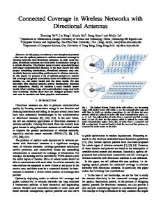
In this section, the performance of the proposed kriging approach is first compared to the radial basis function ANN approach of Nasereddin et al. (2005) and then to the backpropagation ANN approach described in Section 5 in a rigorous experimental study. These two ANN approaches are called RANN and BANN, respectively, to distinguish them in this section. In the experiments, a WLAN with three APs was simulated over an area of 100×100 m2 including different types of walls as shown in Figure 1. To generate a dataset, the area was divided into 50×50 grids and path loss values were sampled at all intersection points of the grids (a total of 2,601 data points). Then, the data points were randomly divided into two sets as training set P (i.e., the set of points where the path loss value is assumed to be surveyed) and test set Q (i.e., the set of points where the path loss value is not known). Let ρ be the probability of selecting a data point as a training point in set P in the process of randomly partitioning data points into sets P and Q. For example, a set of random training points sampled with ρ = .05 are marked by (y) on the target area given in Figure 1. The goal is to estimate the path loss values for test points in set Q using training points in set P. Figure 1
Simulated WLAN coverage over 100 × 100 m2 area
Notes: The area was divided into 50 × 50 grids. The path loss values at the corners of the grids were calculated using the empirical model given in (3) with parameters: L0 = 40.2, c = 4.2, and Lr ranges from 3 to 15. Walls are shown by back lines, and the thickness of a wall indicates its path loss factor. Training points that are randomly selected with ρ = .05 are marked by (y).
First, the RANN approach of Nasereddin et al. (2005) and the kriging approach were compared for different levels of ρ ranging from 0.02 to 0.1. For each level of ρ, 20 random sets of training and test points were generated, and the path loss values at test points were estimated by both RANN and the kriging approaches. In the kriging approach, five nearest training points were used. In the RANN approach, 20 different neural network models were trained for each case by setting the spread parameter of the radial basis layer from 0 to 2.0 by 0.1 intervals, and the model with the smallest estimation error was used in the comparison. The mean absolute percent errors of the kriging and the RANN approaches are compared in Figure 2. In this figure each box plot includes 20 data points (i.e., random training and testing sets), and the same training and testing sets were used in the kriging and neural network approaches for each case. As shown in Figure 2, the kriging approach outperformed the RANN approach of Nasereddin et al. (2005) significantly. In the comparisons given by Konak (2009), the performance of this RANN is at par with the kriging approach. However, the test problem in this paper includes obstacles, making the coverage surface much more complex than the test problems used in Konak (2009). Therefore, the RANN performed poorly particularly for the cases with limited number of training samples. Figure 2
The box plot of mean absolute percent error achieved by the RANN approach (N) and the ordinary kriging approached (O) on 20 random sets of P and Q for various levels of ρ
The BANN and the kriging approaches were also compared for different levels of ρ ranging from 0.02 to 0.1 using five nearest training points as shown in Figure 3. After initial experiments, a network topology with two hidden layers was selected for the BANN in this paper. The network had 15 neurons in the first hidden layer and ten in the second layer (i.e., the topology of the network was 12-15-10-1).
Predicting coverage in wireless local area networks with obstacles using kriging and neural networks The network was trained by the resilient backpropagation algorithm of the MATLAB Neural Network Toolbox for a maximum of 200 epochs. The default settings were used for the training schedule and the neuron activation functions in all layers. All points in set P were used to train the network (i.e., unlike the default setting in the MATLAB Neural network toolbox, the training set was not partitioned into training, validation, and test sets), and the path losses of points in set Q were estimated using the trained network. As seen in Figure 3, the performance of the BANN approach was closer to the kriging approach, but the kriging still provided much more accurate estimations than the BANN approach in this paper. The results in Figures 2 and 3 clearly demonstrate that the kriging approach can outperform neural networks, even universal approximator neural networks such as the BANN proposed in this paper, in estimating wireless network coverage. Figure 3
7
The box plot of mean absolute percent error achieved by the BANN approach (N) and the ordinary kriging approached (O) on 20 random sets of P and Q for various levels of ρ
Conclusions
This paper introduces ordinary kriging as a new tool to predict network coverage in WLANs based on available samples taken in an active site survey. The proposed approach can also be used to validate samples taken during a site survey. In addition, a distance measure is proposed to count the effect of obstacles on the spatial covariance among points. This distance measure has been shown to be effective. The proposed approach can be easily embedded within a site survey computer programme to interpolate signal coverage for points which are not surveyed in the target area. As further research, it will be interesting to
229
integrate the proposed kriging approach into other approaches such as ANNs.
References Andersen, J.B., Rappaport, T.S. and Yoshida, S. (1995) ‘Propagation measurements and models for wireless communications channels’, IEEE Communications Magazine, Vol. 33, No. 1, pp.42–49. Anderson, C.R. and Rappaport, T.S. (2004) ‘In-building wideband partition loss measurements at 2.5 and 60 GHz’, IEEE Transactions on Wireless Communications, Vol. 3, No. 3, pp.922–988. Anderson, C.R., Rappaport, T.S., Bae, K., Verstak, A., Ramakrishnan, N., Tranter, W.H., Shaffer, C.A. and Watson, L.T., (2002) ‘In-building wideband multipath characteristics at 2.5 and 60 GHz’, Proceedings of the IEEE 56th Vehicular Technology Conference, Piscataway, NJ, USA, pp.97–101. Badman, L. (2006) ‘Visualize your WLAN [Ekahau’s site survey 2.2]’, Network Computing, Vol. 17, No. 16, pp.38–39. Bailey, T. and Gatrell, T. (1996) Interactive Spatial Data Analysis, Prentice Hall, Harlow, England. Chen, Y. and Kobayashi, H. (2002) ‘Signal strength based indoor geolocation’, Proceedings of 2002 IEEE International Conference on Communications, New York, NY, USA, pp.436–439. Cheung, K.W., Sau, J.H.M. and Murch, R.D. (1998). ‘A new empirical model for indoor propagation prediction’, IEEE Transactions on Vehicular Technology, Vol. 47, No. 3, pp.996–1001. Funahashi, K. (1989) ‘On the approximate realization of continuous mappings by neural networks’, Neural Networks, Vol. 2, No. 3, pp.183–192. Hata, M. (1980) ‘Empirical formula for propagation loss in land mobile radio services’, IEEE Transactions on Vehicular Technology, Vol. t-29, No. 3, pp.317–325. Hills, A. (2001) ‘Large-scale wireless LAN design’, IEEE Communications Magazine, Vol. 39, No. 11, pp.98–107. Hills, A. and Schlegel, J. (2004) ‘Rollabout: a wireless design tool’, IEEE Communications Magazine, Vol. 42, No. 2, pp.132–138. Hornik, K., Stinchcombe, M. and White, H. (1989) ‘Multilayer feedforward networks are universal approximators’, Neural Networks, Vol. 2, No. 5, pp.359–366. Issaks, E.H. and Srivastava, R.M. (1989) An Introduction to Applied Geostatistics, Oxford University Press, New York, USA. Konak, A. (2009) ‘A kriging approach to predicting coverage in wireless networks’, International Journal of Mobile Network Design and Innovation, Vol. 3, No. 2, pp.64–70. Konak, A. (2010) ‘Estimating path loss in wireless local area networks using ordinary kriging’, Proceedings of Winter Simulation Conference 2010, Baltimore, MD, 5–10 December, pp.2888–2896. Krige, D.G. (1951) ‘A statistical approach to some basic mine valuation problems on the Witwatersrand’, Journal of the Chemical, Metallurgical and Mining Society of South Africa, Vol. 52, No. 6, pp.119–139. Matheron, G. (1963) ‘Principles of geostatistics’, Economic Geology, Vol. 58, No. 8, pp.1246–1266.
230
A. Konak
Nasereddin, M., Konak, A. and Bartolacci, M.R. (2005) ‘A neural network-based approach for predicting connectivity in wireless networks’, International Journal of Mobile Network Design and Innovation, Vol. 1, No. 1, pp.18–23. Neskovic, A., Neskovic, N. and Paunovic, D. (2000) ‘Indoor electric field level prediction model based on the artificial neural networks’, IEEE Communications Letters, Vol. 4, No 6, pp. 190-192. Okumura, Y. and Ohmori, E. (1967) ‘Field strength and its variability in land mobile radio propagation’, Electronics and Communications in Japan, Vol. 50, No. 11, pp.69–79.
Okumura, Y., Ohmori, E., Kawano, T. and Fukuda, K. (1968) ‘Field strength and its variability in VHF and UHF land-mobile radio service’, Review of the Electrical Communication Laboratory (Tokyo), Vol. 16, Nos. 9–10, pp.825–873. Sarkar, T.K., Zhong, J., Kyungjung, K., Medouri, A. and Salazar-Palma, M. (2003) ‘A survey of various propagation models for mobile communication’, IEEE Antennas and Propagation Magazine, Vol. 45, No. 3, pp.51–82. Zvanovec, S., Pechac, P. and Klepal, M. (2003) ‘Wireless LAN networks design: site survey or propagation modeling?’, Radioengineering, Vol. 12, No. 4, pp.42–49.