Connectivity of Growing Random Networks

Connectivity of Growing Random Networks P. L. Krapivsky1,2, S. Redner1 , and F. Leyvraz3

arXiv:cond-mat/0005139v2 [cond-mat.stat-mech] 18 Sep 2000

1

Center for BioDynamics, Center for Polymer Studies, and Department of Physics, Boston University, Boston, MA, 02215 2 CNRS, IRSAMC, Laboratoire de Physique Quantique, Universite’ Paul Sabatier, 31062 Toulouse, France 3 Centro Internacional de Ciencias, Cuernavaca, Morelos, Mexico A solution for the time- and age-dependent connectivity distribution of a growing random network is presented. The network is built by adding sites which link to earlier sites with a probability Ak which depends on the number of pre-existing links k to that site. For homogeneous connection kernels, Ak ∼ kγ , different behaviors arise for γ < 1, γ > 1, and γ = 1. For γ < 1, the number of sites with k links, Nk , varies as stretched exponential. For γ > 1, a single site connects to nearly all other sites. In the borderline case Ak ∼ k, the power law Nk ∼ k−ν is found, where the exponent ν can be tuned to any value in the range 2 < ν < ∞. PACS numbers: 02.50.Cw, 05.40.-a, 05.50.+q, 87.18.Sn

links to an existing site with k links (k − 1 incoming and 1 outgoing). We will solve for the connectivity distribution Nk (t), defined as the average number of sites with k links as a function of the connection kernel Ak . We focus on a class of homogeneous connection kernels, Ak = k γ , with γ ≥ 0 reflecting the tendency of preferential linking to popular sites. As we shall show, the connectivity distribution crucially depends on whether γ smaller than, larger than, or equal to unity. For γ < 1, the connectivity distribution decreases as a stretched exponential in k. The case γ > 1 leads to phenomenon akin to gelation [19] in which a single “gel” site connects to nearly every other site of the graph. For γ > 2, this phenomenon is so extreme that the number of connections between other sites is finite in an infinite graph. A power law distribution Nk ∼ k −ν arises only for γ = 1. In this case, finer details of the dependence of the connection kernel on k affect the exponent ν. Hence we consider a more general class of asymptotically linear connection kernels, Ak ∼ k as k → ∞. We show that ν is tunable to any value in the range 2 < ν < ∞. In particular, we can naturally generate values of ν between 2 and 3, as observed in the web graph [10–12] and in movie actor collaboration networks [13]. The rate equations for the time evolution of the connectivity distribution Nk (t) are

Random networks play an important role in epidemiology, ecology (food webs), and many other fields. The geometry of such fixed topology networks have been extensively investigated [1–7]. However, networks based on human interactions, such as transportation systems, electrical distribution systems, biological systems, and the Internet are open and continuously growing and new approaches are rapidly developing to understand their structure and time evolution [8–12]. In this Letter, we apply a rate equation approach to solve the growing random network (GRN) model, a special case of which was introduced in [13] to account for the distribution of citations and other growing networks [13–18]. Our approach is ideally-suited for the GRN and is much simpler than the standard probabilistic [1] or generating function [2] techniques. The rate equation formulation can be adapted to study more general evolving graph systems, such as networks with site deletion and link re-arrangement. 9 8

1

4

7 6

10

3

2

dNk 1 [(k − 1)γ Nk−1 − k γ Nk ] + δk1 . = dt Mγ

5

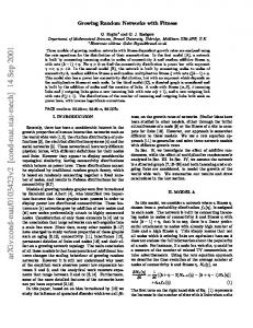
FIG. 1. Schematic illustration of the evolution of the growing random network. Sites are added sequentially and a single link joins the new site to an earlier site.

(1)

The first term accounts for the process in which a site with k − 1 links is connected to the new site, leading to a gain in the number of sites with k links. This Phappens with probability (k − 1)γ /Mγ , where Mγ (t) = j γ Nj (t) provides the proper normalization. A corresponding role is played by the second (loss) term on the right-hand side of Eq. (1). The last term accounts for the continuous introduction of new sites with no incoming links. We start by finding the low-order moments Mn (t) of the connectivity distribution. Summing Eqs. (1) over all k gives the rate equation for the total number of sites, M˙ 0 = 1, whose solution is M0 (t) = M0 (0) + t. The first moment (the total number of bond endpoints) obeys

The GRN model is defined as follows. At each time step, a new site is added and a directed link to one of the earlier sites is created. In terms of citations, we may interpret the sites in Fig. 1 as publications, and the directed link from one paper to another as a citation to the earlier publication. This growing network has a directed tree graph topology where the basic elements are sites which are connected by directed links. The structure of this graph is determined by the connection kernel Ak , which is the probability that a newly-introduced site 1

M˙ 1 = 2, which gives M1 (t) = M1 (0) + 2t. The first two moments are therefore independent of γ, while higher moments and the connectivity distribution itself do depend on γ. For the linear connection kernel, Eqs. (1) can be solved for an arbitrary initial condition. We limit ourselves to the most interesting asymptotic regime (t → ∞) where the initial condition is irrelevant. Using M1 = 2t, we solve the first few of Eqs. (1) and obtain N1 = 2t/3, N2 = t/6, etc., which implies that the Nk grow linearly with time. Accordingly, we substitute Nk (t) = t nk in Eqs. (1) to yield the recursion relation nk = nk−1 (k − 1)/(k + 2). Solving for nk then gives nk =

4 . k(k + 1)(k + 2)

To complete the solution for the nk , we need to establish the dependence of the amplitude µ on γ. Using the P defining relation Mγ /t = µ = k≥1 k γ nk , together with Eq. (4), we obtain the implicit relation for µ(γ) −1 ∞ Y k  X µ . 1+ γ µ= j j=2

Despite the simplicity of this exact expression, it is not easy to extract explicit information except for the limiting cases γ = 0 and γ = 1, where µ = 1 and µ = 2 respectively, and the corresponding connectivity distributions are given by nk = 2−k and by Eq. (2). However, numerical evaluation shows that µ varies smoothly between 1 and 2 as γ increases from 0 to 1 (Fig. 2). This result, together with Eq. (4), provides a comprehensive description of the connectivity distribution in the regime < 0 ≤ γ ≤ 1. It is worth emphasizing that for 0.8 < ∼ γ ∼ 1, nk depends weakly on γ for 1 ≤ k ≤ 1000. Thus, it is difficult to discriminate between different γ’s and even to distinguish a power law from a stretched exponential in the GRN model. This subtlety was already encountered in the analysis of the citation distribution [15,16]. A striking feature of the GRN model is that we can “tune” the exponent ν by augmenting the linear connection kernel to the asymptotically linear connection kernel, with Ak → a∞ k as k → ∞, but otherwise arbitrary. For this asymptotically linear kernel, by repeating the steps leading to Eq. (4) we find

(2)

To solve the model with a sub-linear connection kernel, 0 < γ < 1, notice that Mγ satisfies the obvious inequalities M0 ≤ Mγ ≤ M1 . Consequently, in the long-time limit Mγ = µt,

1 ≤ µ ≤ 2,

(3)

with a yet undetermined prefactor µ = µ(γ). Now substituting Nk (t) = t nk and Mγ = µt into Eqs. (1) and again solving for nk we obtain −1 k  µ µ Y 1+ γ , nk = γ k j=1 j

(4)

whose asymptotic behavior is  h  1−γ 1−γ i −2 1  k −γ exp −µ k 1−γ  2 < γ < 1,     µ2 −1 h √ i nk ∼ k 2 exp −2µ k (5) γ = 21 ,    i h   1 1  k −γ exp −µ k1−γ + µ2 k1−2γ 1−γ 2 1−2γ 3 < γ < 2,

−1 k  µ µ Y 1+ nk = . Ak j=1 Aj

µ = A1

µ

1.6 1.4 1.2

0.4

γ

0.6

0.8

µ 1+ Aj

−1

.

(8)

As an explicit example, consider the connection kernel A1 = 1 and Ak = a∞ k for k ≥ 2. In this case, we can reduce Eq. (8)p to a quadratic equation from which we obtain ν = (3 + 1 + 8/a∞ )/2 which can indeed be tuned to any value larger than 2. The GRN model with super-linear connection kernels, γ > 1, exhibits a “winner take all” phenomenon, namely the emergence of a single dominant “gel” site which is linked to almost every other site. A particularly singular behavior occurs for γ > 2, where there is a non-zero probability that the initial site is connected to every other site of the graph. To determine this probability, it is convenient to consider a discrete time version process where one site is introduced at each step which always links to the initial site. After N steps, the probability that the

1.8

0.2

∞ Y k  X k=2 j=2

2

0

(7)

Expanding the product in Eq. (7) leads to nk ∼ k −ν with ν = 1 + µ/a∞ , while the amplitude µ is found from

etc. This pattern in (5) continues ad infinitum: Whenever γ decreases below 1/m, with m a positive integer, an additional term in the exponential arises from the now relevant contribution of the next higher-order term in the expansion of the product in Eq. (4).

1

(6)

k=2

1

FIG. 2. The amplitude µ in Mγ (t) = µt versus γ.

2

new site will link to the initial site is N γ /(N + N γ ). This pattern continues indefinitely with probability P=

∞ Y

N =1

1 . 1 + N 1−γ

Thus for super-linear kernels, the GRN undergoes an infinite sequence of connectivity transitions as a function of γ. For γ > 2 all but a finite number of sites are linked to the “gel” site which has the rest of the links of the network. This is the “winner take all” situation. For 3/2 < γ < 2, the number of sites with two links grows as t2−γ , while the number of sites with more than two links is again finite. For 4/3 < γ < 3/2, the number of sites with three links grows as t3−2γ and the number with m more than three is finite. Generally for m+1 m < γ < m−1 , the number of sites with more than m links is finite, while Nk ∼ tk−(k−1)γ for k ≤ m. Logarithmic corrections also arise at the transition points. The connectivity distribution leads to an amusing consequence for the most P popular site. Its connectivity kmax is determined by k>kmax Nk = 1, that is, there is one site whose connectivity lies in the range (kmax , ∞). This criterion gives   (ln t)1/(1−γ) 0 ≤ γ < 1; kmax ∼ t1/(ν−1) (13) asymptotically linear;  t super-linear.

(9)

Clearly, P = 0 when γ ≤ 2 but P > 0 when γ > 2. Thus for γ > 2 there is a non-zero probability that the initial site connects to all other sites. To determine the behavior for general γ > 1, we need the asymptotic time dependence of Mγ . To this end, it is useful to consider the discretized version of the master equations Eq. (1), where the time t is limited to integer values. Then Nk (t) = 0 whenever k > t and the rate equation for Nk (k) immediately leads to Nk (k) =

(k − 1)γ Nk−1 (k − 1) Mγ (k − 1)

= N2 (2)

k−1 Y j=2

jγ . Mγ (j)

(10)

Since t also equals the total number of sites, we can compare this prediction about the most popular site with available data from the Institute of Scientific Information based on 783,339 papers with 6,716,198 total citations (details in Ref. [16]). Here the most cited paper had 8,904 citations. This accords with the first line of Eq. (13) for γ ≈ 0.86, and also with the second when ν ≈ 2.5. In addition to the connectivity of a site, we also may ask about its age. Within the GRN model, older sites should clearly be more highly connected. We quantify this feature and also determine how the connection kernel affects the combined age and connectivity distribution. Note that our model does not have explicit aging where the connection kernel depends on the age of each site; this feature is treated in Ref. [17]. Let ck (t, a) be the average number of sites of age a which have k − 1 incoming links at time t. Here age a means that the site was introduced at time t − a. The quantity ck (t, a) evolves according to

From this and the obvious fact that Nk (k) must be less than unity, it follows that Mγ (t) cannot grow more slowly than tγ . On the other hand, Mγ (t) cannot grow faster than tγ as follows from the estimate Mγ (t) =

t X

k γ Nk (t)

k=1

≤ tγ−1

t X

kNk (t) = tγ−1 M1 (t)

(11)

k=1

Thus Mγ ∝ tγ . In fact, the amplitude of tγ is unity as will be derived self-consistently after solving for the Nk ’s. We now use Mγ ∼ tγ in the rate equations to solve recursively for each Nk . Starting with the equation N˙ 1 = 1 − N1 /Mγ , the second term on the right-hand side is sub-dominant; neglecting this term gives N1 = t. Continuing this same line of reasoning for each successive rate equation gives the leading behavior of Nk , Nk = Jk tk−(k−1)γ

for k ≥ 1,

(12)

∂ck 1 ∂ck [(k − 1)γ ck−1 − k γ ck ] + δk1 δ(a). (14) + = ∂t ∂a Mγ

Qk−1 with Jk = j=1 j γ /[1 + j(1 − γ)]. This pattern of behavior for Nk continues as long as its exponent k − (k − 1)γ remains positive, or k < γ/(γ − 1). The full behavior of the Nk may be determined straightforwardly by keeping the next correction terms in the rate equations. For example, N1 = t − t2−γ /(2 − γ) + . . .. For k > γ/(γ − 1), each Nk has a finite limiting value in the long-time limit. Since the total number of connections equals 2t and t of them are associated with N1 , the remaining t links must all connect to a single site which has t connections (up to corrections which grow no faster than sub-linearly with time). Consequently the amplitude of Mγ equals unity, as argued above.

The second term on the left-hand side accounts for the aging of sites, while the right-hand side accounts for the (age independent) connection changing processes. Consider first the linear kernel, Ak = k. Let us focus again on the most interesting limit, namely asymptotic behavior. Then we can disregard the initial condition and write M1 (t) = 2t. This transforms Eqs. (14) into   ∂ ∂ (k − 1)ck−1 − kck + + δk1 δ(a). (15) ck = ∂t ∂a 2t The homogeneous form of this equation suggests that solution should be self-similar. Specifically, one can seek 3

a solution as a function of the single variable a/t rather than two separate variables, ck (t, a) = fk (a/t). This simplifies the partial differential equation (15) into an ordinary differential equation for fk (x) which can be easily solved. In terms of the original variables of a and t, we find r r  k−1 a a 1− 1− . (16) ck (t, a) = 1 − t t

port. While writing this manuscript we learned of Ref. [20] which overlaps some of our results. We thank J. Mendes for informing us of this work.

[1] B. Bollob´ as, Random Graphs (Academic Press, London, 1985). [2] S. Janson, T. Luczak, and A. Rucinski, Random Graphs (Wiley, New York, 2000). [3] S. A. Kauffman, The Origin of Order: Self-Organization and Selection in Evolution (Oxford University Press, London, 1993). [4] S. Wasserman and K. Faust, Social Network Analysis (Cambridge University Press, Cambridge, 1994). [5] B. Derrida and H. Flyvbjerg, J. Physique 48, 971 (1987). [6] H. Flyvbjerg and N. J. Kjaer, J. Phys. A 21, 1695 (1988). [7] U. Bastolla and G. Parisi, Physica D 98, 1 (1996). [8] R. V. Sol´e and S. C. Manrubia, Phys. Rev. E 54, R42 (1996). [9] S. Jain and S. Krishna, Phys. Rev. Lett. 81, 5684 (1998). [10] J. Kleinberg, R. Kumar, P. Raphavan, S. Rajagopalan, and A. Tomkins, in: Proc. Inter. Conf. on Combinatorics and Computing (1999). [11] S. R. Kumar, P. Raphavan, S. Rajagopalan, and A. Tomkins, in: Proc. 25th VLDB Conf. (1999). [12] A. Broder, R. Kumar, F. Maghoul, P. Raphavan, S. Rajagopalan, R. Stata, A. Tomkins, and J. Wiener, in: Proc. 9th WWW Conf. (2000). [13] A. L. Barab´ asi and R. Albert, Science 286, 509 (1999). [14] A. J. Lotka, J. Washington Acad. Sci. 16, 317 (1926); W. Shockley, Proc. IRE 45, 279 (1957). [15] J. Lahererre and D. Sornette, Eur. Phys. J. B 2, 525 (1998). [16] S. Redner, Eur. Phys. J. B 4, 131 (1998). [17] S. N. Dorogovtsev and J. F. F. Mendes, Phys. Rev. E 62, 1842 (2000). [18] B. A. Huberman, P. L. T. Pirolli, J. E. Pitkow, and R. Lukose, Science 280, 95 (1998); S. M. Maurer and B. A. Huberman, nlin.CD/0003041. [19] M. H. Ernst, in Fundamental Problems in Stat. Physics VI, ed. E. G. D. Cohen (Elsevier, New York, 1985). [20] S. N. Dorogovtsev, J. F. F. Mendes, and A. N. Samukhin, cond-mat/0004434. [21] P. L. Krapivsky and S. Redner, (preprint).

Notice that this age distribution R t satisfies the normalization requirement, Nk (t) = 0 da ck (t, a). As expected, young sites (those with a/t → 0) typically have a small connectivity while old sites have large connectivity. Further, old sites have a broad distribution of connectivities up to a characteristic number which asymptotically grows as hki ∼ (1 − a/t)−1/2 as a → t. These properties and related issues may be worthwhile to investigate in citation and other information networks. Similarly, we can obtain ck (t, a) for the GRN model with an arbitrary homogeneous connection kernel [21] which grows slower than linearly in k. Assuming a selfsimilar solution ck (t, a) = fk (a/t), applying a Laplace transform, we find a recursion relation for fˆk whose solution is identical in structure to Eq. (4). Although it appears impossible to perform the inverse Laplace transform in explicit form for arbitrary k, we can compute ck (t, a) for small k; for example, we find c1 = (1−a/t)1/µ . The behavior also simplifies in the large-k limit. Here we find that the age of sites with k links is peaked about the value ak which satisfies   ( 1−γ γ < 1; 1 − exp −µ k1−γ ak (17) ≃ 12 t 1− γ = 1. (k+3)(k+4)

This shows how old sites are better connected. In summary, we solved for both the connectivity distribution and the age-dependent structure of the growing random network. The most interesting connectivity arises in a network with an asymptotically linear connection kernel. Here the number of sites with k connections has the power-law form Nk ∼ k −ν , with ν tunable to any value in the range 2 < ν < ∞. This accords with the connectivity distributions observed in various contemporary examples of growing networks. We are grateful to grants NSF INT9600232, NSF DMR9978902, and DGAPA IN112998 for financial sup-

4