2010 IEEE Information Theory Workshop - ITW 2010 Dublin
Constrained Codes for Phase-change Memories Anxiao (Andrew) Jiang
Jehoshua Bruck
Hao Li
Computer Science and Eng. Dept. Texas A&M University College Station, TX 77843 Email:
[email protected]
Electrical Engineering Department California Institute of Technology Pasadena, CA 91125 Email:
[email protected]
Computer Science and Eng. Dept. Texas A&M University College Station, TX 77843 Email:
[email protected]
Abstract—Phase-change memories (PCMs) are an important emerging non-volatile memory technology that uses amorphous and crystalline cell states to store data. The cell states are switched using high temperatures. As the semi-stable states of PCM cells are sensitive to temperatures, scaling down cell sizes can bring significant challenges. We consider two potential thermal-based interference problems as the cell density approaches its limit, and study new constrained codes for them.
0
1
2
3
Fig. 1. The transitions among q cell levels. (Here q = 4.) The forward and backward edges represent the SET and RESET operations, respectively.
I. I NTRODUCTION Phase-change memories (PCMs) are an important emerging non-volatile memory (NVM) technology. Its basic storage unit, a PCM cell, has at least two states: the amorphous state and the crystalline state. To achieve higher storage capacity, multilevel cells (MLCs) are being developed, where additional partially crystalline states are used [1]. We model the q ≥ 2 states of a PCM cell by q levels – levels 0, 1, . . . , q − 1 – where level 0 is the amorphous state, level 1, . . . , q − 2 are the partially crystalline states, and level q − 1 is the crystalline state. As a cell becomes more crystallized, its level increases. The level of a PCM cell is switched using high temperatures. A cell can be heated by a high cell-melting temperature (about 600o C ∼ 700o C) to change to level 0 (amorphous state), or be heated by a more moderate temperature to increase its level (i.e., to a more crystallized state). To model the direct switching of states, we use the diagram in Fig. 1 (for q = 4 as an example) [3]. We see that the cell can be changed from any level i ∈ {1, 2, . . . , q − 1} directly to level 0 (called a RESET operation), and from any level i directly to level j for 0 ≤ i < j ≤ q − 1 (called a SET operation). However, for 0 < j < i ≤ q − 1, to change it from level i to level j, both the RESET and SET operations are needed. PCMs are under active study and development due to their very attractive potentials. Compared to the widely used flash memories, PCMs can potentially scale to much smaller cell sizes and achieve higher storage capacity. They can also have substantially better endurance, data retention and read/write speed [1]. However, scaling down cell sizes can also bring significant challenges, and solving them will be key to the PCM development [1]. A major and widely acknowledged challenge is the thermal issue, because the amorphous and partially-crystalline states are only semi-stable states, and high environmental temperatures can further crystalize the cell, i.e., unintentionally increase the cell level [1], [5]. We consider two potential challenges when the PCM’s cell
density scales toward its limit. The first one is the thermal crosstalk problem, namely, when a cell is RESET (to level 0) by the high melting temperature, the heat affects its adjacent cell and makes it further crystalized [1], [5]. Note that this may happen both when the adjacent cell is not being programmed and when it is being SET, unless it is already in the fully crystalized state (level q − 1). It is because in both cases, the semi-stable cell state is sensitive to high temperatures. The second problem is the local thermal accumulation problem. When cells are repeatedly programmed, the heat can accumulate in the area [5]. This residual heat can be a major factor that limits the writing bandwidth of PCMs, because the writing accuracy is sensitive to temperature [1], [5]. When the cell density scales toward its limit, relative to the high I/O speed, it can take nontrivial time for the locally generated heat to spread out uniformly in the memory chip. So if an application repeatedly writes a cluster of adjacent cells at very high speed, the accumulated heat may appear localized [5]. In that case, it is worth considering whether there exist schemes that can make the thermal accumulation more balanced. The above problems have been considered in [1], [5] from the device and system perspectives. In this paper, we consider coding techniques for these potential challenges. For the thermal crosstalk problem, we use a scheme that removes the crosstalk interference, and then study coding techniques that reduce the programming cost (measured by the number of RESET operations). For the local thermal accumulation problem, we study coding techniques that impose time and space constraints on writing, to help the heat generated by programming be more balanced spatially. Constrained coding is an important area of coding techniques, and has been applied successfully to both magnetic recording and optical recording [4]. Compared to conventional constrained coding, the codes studied in this paper are for a different setting and sometimes require very different coding
978-1-4244-8263-4/10/$26.00 © 2010 IEEE
techniques. It is also notable that for PCMs, the constraints are not limited to just within a codeword. They are introduced by the difference between old codewords and the new codewords that overwrite them, because only cells that are programmed can generate heat, which may affect other cells. The rest of the paper is organized as follows. In Section II, we present symbol-constrained codes for the thermal crosstalk problem. In Section III, we present space-time constrained codes for the local thermal accumulation problem. In Section IV, we present the concluding remarks. Due to space limitation, we leave some detailed analysis in the full paper [2]. II. S YMBOL - CONSTRAINED C ODES In this section, we study coding techniques for the thermal crosstalk problem. Let c1 , c2 , . . . , cn be n cells. For i ∈ {1, 2, . . . , n} , [n], let ℓi ∈ {0, 1, . . . , q − 1} denote the level of ci . In this paper, we consider the cells as a onedimensional array. (The concepts can be extended to higher dimensions, too.) Two cells ci and cj are neighbors if and only if |i − j| = 1. Let γ ∈ {1, 2, . . . , q − 1} be a parameter. We consider the following simple model for thermal crosstalk: When a cell ci is RESET to level 0, the thermal crosstalk from ci (at that moment) will increase its neighboring cell’ level ℓj (for j = i ± 1) by at most γ, unless the neighboring cell cj is also being RESET at that moment. (However, a cell level cannot exceed q − 1, the stable fullycrystalline state. And a SET operation does not affect the neighboring cells due to its considerably lower temperature.) Let C ⊆ {0, 1, . . . , q − 1}n be a code, whose rate R(C) is defined as logn2 |C| . (Clearly, R(C) ≤ log2 q.) A rewrite is to change the cell levels from the current codeword X = (x1 , . . . , xn ) ∈ C to a new codeword Y = (y1 , . . . , yn ) ∈ C. For i ∈ [n], if xi > yi , then the rewrite needs to RESET ci (and then SET ci if yi > 0). For j = i ± 1, if ci is RESET and yj < min{xj + γ, q − 1}, then the rewrite needs to RESET cj as well, because otherwise the thermal crosstalk from ci may make ℓj greater than yj . Therefore, a RESET operation applied to a cell can trigger the RESET of its neighboring cell, and this effect can propagate to many cells. Let us define a RESET segment in codeword Y as a maximum run of symbols yi , yi+1 , . . . , yj (where 1 ≤ i ≤ j ≤ n) such that: (1) ∀ i′ ∈ {i, . . . , j}, yi′ < min{xi′ +γ, q−1}; (2) ∃ i′′ ∈ {i, . . . , j} such that xi′′ > yi′′ . By our above analysis, the rewrite must RESET all the cells in a RESET segment (before setting them). To rewrite cells using parallel programming, it is natural to use the following two-step procedure: First, RESET all the cells in RESET segments of the new codeword; then, SET all the cells whose levels are still lower than their values in the new codeword. (The second step has no crosstalk effect.) Example 1. Let n = 11, q = 4 and γ = 3. Assume the cells need to change from an old codeword (1, 3, 2, 2, 2, 2, 2, 2, 1, 1, 1) to a new codeword (0, 3, 2, 2, 1, 2, 2, 2, 3, 1, 2). First, we RESET the cells {c1 , c3 , c4 , c5 , c6 , c7 , c8 }. (After this step, the cell levels will be (0, 3, 0, 0, 0, 0, 0, 0, ℓ9 , 1, 1), where ℓ9 ∈ {1, 2, 3}. (Since
cell c8 is RESET, the thermal crosstalk from c8 may make ℓ9 be greater than its original value 1.) Then, we SET the cells {c3 , c4 , c5 , c6 , c7 , c8 , c9 , c11 }, to increase the cell levels to (0, 3, 2, 2, 1, 2, 2, 2, 3, 1, 2). We define the cost of a rewrite operation as the number of cells that are RESET during rewriting. (In Example 1, the cost is 7.) The number of RESETs is a very important cost measurement because PCM cells have a limited longevity: PCM cells can endure about 106 ∼ 108 RESETs (or SET-RESET cycles) before becoming non-functional [1], [3]. Note that for the rewrite, for every cell that needs to decrease its level, the whole RESET segment containing it is forced (triggered) to be RESET, too. This motivates us to study constrained codes where RESET segments have limited lengths. Given this constraint, we seek capacity-achieving codes. In this paper, we focus on the case γ = q − 1 (the worstcase scenario for thermal crosstalk). We define an unstable segment in a codeword X = (x1 , . . . , xn ) as a maximum run of symbols xi , xi+1 , . . . , xj (where 1 ≤ i ≤ j ≤ n) such that for i′ ∈ {i, . . . , j}, xi′ < q − 1. The length of this unstable segment is j − i + 1. When the memory writes X, an unstable segment in it will become a RESET segment if any of the cells in that unstable segment needs to decrease its level (compared to the old codeword). For a code C, if in all its codewords the unstable segments’ lengths are at most k, then during rewriting, the length of every RESET segment is at most k. Definition 2. S YMBOL - CONSTRAINED CODES Let k be a positive integer. A code C ⊆ {0, 1, . . . , q − 1}n is k -limited if in every codeword of C , every unstable-segment’s length is at most k . (It is also called a symbol-constrained code.) The k-limited codes are a constrained system S over alphabet Σ , {0, 1, . . . , q − 1}. An example for q = 4, k = 3 is shown in Fig. 2. We see that it generalizes the (d = 0, k)run-length-limited (RLL) codes [4] from the binary alphabet to the q-ary alphabet. Its Shannon capacity is cap(S) = limn→∞ sup n1 log N (n; S), where N (n; S) is the number of words of length n in S. We have constructed a k-limited code for q = 4 and k = 1, which has a rate 6 : 5 finite-state encoder. Its rate is 1.2 bits/cell, close to the Shannon capacity (which can be shown to be 1.203). When the code is used for storing data, assuming that the input information bits have a uniform i.i.d. distribution, for every rewrite, the ratio of the average number of RESET operations to the number of information bits is 0.228. This compares favorably with the no-coding method (i.e., storing 2 bits per cell), which has a higher ratio of 0.345. So symbol-constrained codes can reduce RESETs. (For more details of the code, see [2].) We note that rewriting codes for reducing the RESET operations for PCMs have been studied in [3], where interesting WOM-like codes have been used. However, the study in [3] did not consider any thermal interference problem. We also stress that the codes in [3] and the codes we study are two drastically different approaches. While the codes in [3] always RESET
3 0
0
0
0
1
1
1
2
2
2
1
3
2 3
3 3
Fig. 2. Shannon cover of the 3-limited codes (constrained system), for q = 4. TABLE I S HANNON C APACITY ( BITS PER CELL ) OF k- LIMITED CODES q\k
1
2
3
4
5
6
2 3 4 5 6 7 8 9 10 11 12 13 14 15 16
0.694 1.000 1.203 1.357 1.481 1.585 1.675 1.754 1.824 1.888 1.946 2.000 2.050 2.096 2.139
0.879 1.303 1.585 1.797 1.968 2.111 2.234 2.342 2.438 2.525 2.604 2.677 2.745 2.807 2.866
0.947 1.432 1.756 2.000 2.196 2.360 2.501 2.624 2.734 2.834 2.924 3.008 3.084 3.156 3.223
0.975 1.496 1.846 2.110 2.322 2.499 2.651 2.785 2.904 3.011 3.108 3.198 3.281 3.358 3.430
0.988 1.531 1.899 2.176 2.399 2.585 2.745 2.885 3.010 3.123 3.225 3.319 3.406 3.487 3.563
0.994 1.552 1.931 2.218 2.449 2.642 2.807 2.953 3.082 3.199 3.305 3.402 3.492 3.576 3.654
all cells at the same time (to get a fresh start for rewriting), we use constrained codes that are based on local constraints, and cells are most likely RESET in different rewrites. And with our constrained-coding approach, slide-block decoders can be built to locally decode information bits efficiently. The following theorem presents the Shannon capacity of the symbol-constrained codes, for arbitrary q and k. Due to the space limitation, we present its full proof in [2]. Theorem 3. Let q ≥ 2 and k ≥ 1 be integers. Let f (λ) = λk+2 − qλk+1 + (q − 1)k+1 .
The equation f (λ) = 0 has at most three real-valued solutions, one of which is q − 1. Among those real-valued solutions, if q = k + 2, let λ∗ be the solution with the greatest absolute value; otherwise, among the (at most two) real-valued solutions unequal to q − 1, let λ∗ be the solution with the greater absolute value. Then the Shannon capacity of k -limited codes is log2 |λ∗ | bits per cell. Based on Theorem 3, the Shannon capacity of symbolconstrained codes for different q and k are shown in Table I. III. S PACE -T IME C ONSTRAINED C ODES In this section, we study coding techniques for a different interference problem: the local thermal accumulation problem. It is known that when cells are repeatedly programmed, adjacent cells can be crystallized/disturbed [5]. We seek codes for rewriting data that can balance heat better. This motivates us to study the space-time constrained codes defined below.
Let c1 , . . . , cn be n PCM cells, whose levels are denoted by ℓ1 , . . . , ℓn ∈ {0, . . . , q − 1}. Let V = {0, 1, . . . , v − 1} be an alphabet of size v. The data stored in the n cells takes its value from the alphabet V . A code C is a mapping from the cell levels L , (ℓ1 , . . . , ℓn ) ∈ {0, . . . , q − 1}n to the data values V . We allow it to be a many-to-one mapping (instead of a oneto-one mapping). The code C has two associated functions: a decoding function Fd and an update function Fu . The decoding function Fd : {0, . . . , q − 1}n → V tells us that the cell levels L represent the data Fd (L) ∈ V . The update function Fu : {0, . . . , q − 1}n × V → {0, . . . , q − 1}n tells us that if the old cell levels are L and we want to write the new data s ∈ V into the cells, we will change the cell levels to Fu (L, s). (Clearly, we should have Fd (Fu (L, s)) = s.) A rewrite can change the data to any value in V . Here we do not consider the thermal crosstalk problem. So when a rewrite changes an old codeword X = (x1 , . . . , xn ) ∈ {0, . . . , q − 1}n to a new codeword Y = (y1 , . . . , yn ), for i ∈ [n], a cell ci needs to be programmed only if xi 6= yi . We define the rewrite cost as the number of cells that are programmed, |{i ∈ [n] | xi 6= yi }|, which is the Hamming distance between X and Y . To balance programming-generated heat, we study the following code.1 Definition 4. S PACE - TIME CONSTRAINED CODES Let α, β, p be positive integers. A code is (α, β, p)constrained if for any α consecutive rewrites and for any segment of β cells – namely, ci , ci+1 , . . . , ci+β−1 for some i ∈ [n] – the total rewrite cost of those β cells (over those α rewrites) is at most p. (It is also called a space-time constrained code.) We note that the space-time constrained codes are interesting because although the system can keep moving data that are frequently rewritten to balance heat, such an approach may cause substantial overhead for file-system/compiler design and their optimization. And for content-addressable systems, where the address of data is determined by the content of the data (e.g., by using a hash function) for fast data retrieval, relocating data can also be very challenging. In this paper, as the starting point of understanding space-time constrained codes, we study the time and space constraints separately. A. Time-constrained Codes We first study time-constrained codes with α ≥ 1, β = 1, p = 1. This is the simple case where every cell can be programmed at most once in every α consecutive rewrites. Note that the rate of the code C is defined as logn2 v bits per cell. It is easy to see that a simple idea based on time division can give us a code of rate logα2 q bits per cell, as follows: Let n = α⌈logq v⌉, and divide the n cells evenly into α groups (call them the 0th, 1st, 2nd, . . . , (α − 1)-th cell groups); for i = 1, 2, 3 · · · , for the i-th rewrite we write the data into the (i mod α)-th cell group. When n → ∞ (which also means 1 The model can be generalized by differentiating the cost of RESET and SET operations. In PCMs, the RESET operation uses a higher temperature that the SET operation, but has a shorter duration of time.
v → ∞), the code rate approaches logα2 q bits per cell. So the question is if there exist codes of higher rates. Note that the challenge for designing time-constrained codes is that we cannot afford to remember for every cell how long ago the cell was programmed for the last time (up to α past rewrites), because that alone will cost log2 α bits of storage space for every cell. (Consider the case q = 2.) So the programming of cells needs to be synchronized in some way so that this information cost can be reduced. We now present a general time-constrained code construction for q = 2 that uses the write-once memory (WOM) codes [6] as sub-codes. Let D be a WOM code that stores data of alphabet size w in m cells of q = 2 levels. Denote the alphabet of the stored data by W = {0, 1, . . . , w − 1}. The code D also has a decoding function Fd(D) : {0, 1}m → W and an update function Fu(D) : {0, 1}m × W → {0, 1}m . WOM codes have a unique property: with every rewrite, the cell levels can only increase, not decrease [6]. Let t denote the number of rewrites the code D can guarantee to support. (Let the initial cell levels all be zero.) Clearly, due to the unique property of WOM codes, t is a finite number. Example 5. Let w = 4, m = 3, q = 2. Let L′ , (ℓ′1 , ℓ′2 , ℓ′3 ) ∈ {0, 1}3 denote the three cell levels. The following WOM code D was presented by Rivest and Shamir [6] with t = 2: L′ Fd(D) (L′ )
000 0
100 1
010 2
001 3
110 3
101 2
011 1
111 0
If the t = 2 rewrites first write the data as 2, the rewrite it as 1, the code will first let L′ be (0, 1, 0), the change it to (0, 1, 1). Let E be an “elevator code” that mimics D but allows the cell levels to increase and decrease in a synchronized way, described as follows. E also stores data of alphabet size w in m cells of q = 2 levels. Plainly speaking, for the first α rewrites, E rewrites data in the same way as D; then it pushes all the m cell levels to q − 1 = 1; for the next α rewrites, E rewrites data by decreasing cell levels, in exactly the opposite way of D; then it pushes all the m cell levels to 0; then the third batch of α rewrites are implemented in the same way as D again; and so on. We now formally define the decoding function Fd(E) and the update function Fu(E) of E. Let us call a sequence of rewrites the 0th, 1st, 2nd, 3rd · · · rewrites. For i = 0, 1, 2 . . . , let L′i denote the cell levels after the i-th rewrite, and let ei ∈ W denote the data that the i-th rewrite writes into the cells. (Clearly, we should have Fd(E) (L′i ) = ei .) Then if 0 ≤ (i mod 2α) ≤ α − 1, Fd(E) (L′i ) = Fd(D) (L′i ); ′ otherwise, Fd(E) (L′i ) =¡ Fd(D) ((q ¢ − 1, · · · , q − 1) − Li ). If ′ i ≡ 0 mod 2α, Fu(E) Li−1 , ei = Fu(D) ((0, ¡ ·′ · · , 0)¢, ei ). If 1 ¡≤ (i mod 2α) ≤ α − 1, F u(E) ¡Li−1 , ei ¢ = ¢ Fu(D) L′i−1 , ei . If i ≡ α mod 2α, Fu(E) L′i−1 , ei = (q − 1, . . . , q − 1) − Fu(D) ((0, · · · , 0)¡, ei ). ¢ If ′ , e α + 1 ≤ (i mod 2α) ≤ 2α − 1, F L u(E) i−1 i ¢ = ¡ (q − 1, . . . , q − 1) − Fu(D) (q − 1, · · · , q − 1) − L′i−1 , ei .
Example 6. Let D be the WOM code in Example 5, and let E be the “elevator code” defined as above. Then when the rewrites change the data as 1 → 2 → 3 → 2 → 3 → 1 → · · · , the code E changes the cell levels as (0, 0, 0) → (1, 0, 0) → (1, 0, 1) → (1, 1, 1) → (1, 1, 0) → (0, 1, 0) → (0, 0, 0) → (0, 0, 1) → (0, 1, 1) → (1, 1, 1) → · · · We now construct the code C that stores data of alphabet t size v in n cells of q = 2 levels. Let v = w gcd(t,α) , where gcd (t, α) is the greatest common divisor of t and m(t+α) . We see the stored data as a vector α. Let n = gcd(t,α) ´ ³ t t ∈ {0, 1, . . . , w − 1} gcd(t,α) . X = x1 , x2 , . . . , x gcd(t,α) For i = 0, 1, 2 · · · , let Xi denote the data (vector) that the i-th rewrite writes into the n cells. We divide the n t+α groups, and call them the 0th, cells evenly into gcd(t,α) 1st, · · · , (gcd (t, α) − 1)-th groups. (Every cell group has m cells.) We implement a sequence rewrites as follows. For i ⌋. Then for the i-th i = 0, 1, 2 . . . , let g(i) = ⌊ gcd(t,α) t rewrite, the gcd(t,α) elements of Xi are, respectively, written ³ ´ ³ ´ t+α t+α into the g(i) mod gcd(t,α) -th, g(i) + 1 mod gcd(t,α) ´ ³ t+α t − 1 mod gcd(t,α) -th cell groups. th, · · · , g(i) + gcd(t,α) (After the rewrite, the data can be decoded from those cell groups as well.) Every cell group uses the “elevator code” E to rewrite data. (For a cell group, after it is used for t consecutive rewrites, all its cell levels will be pushed to zero or q −1 when the next rewrite comes. The it will rest for α − 1 rewrites.) We can see that every cell group will be programmed in t+1 consecutive rewrites, then not programmed for another α − 1 consecutive rewrites, and then repeat this process. In such a period of t+α rewrites, the cell levels are either all increasing or all decreasing; since q = 2, every cell can be programmed only once. So every cell is programmed at most once for every α consecutive rewrites. So C is a time-constrained code. The only detail left to specify is how to know the value of i mod 2(t + α) when the i-th rewrite happens, which is needed in the above coding process. (It is used to compute g(i) and to implement the “elevator code.”) This value can be obtained by using a simple “counter” of 2(t + α) cells of q = 2 levels. Let ℓ′1 , ℓ′2 , . . . , ℓ′2(t+α) denote their levels. We cyclically program the cells; for every ¯rewrite, we change the level of one cell. ¯ P2(t+α)−1 ¯ ′ ¯ We see j=1 ¯ℓj − ℓ′2(t+α) ¯ equals i mod 2(t + α). So we can get the wanted value, and every cell in the counter is programmed exact once for every 2(t + α) > α rewrites. Let w → ∞, fix t as a constant, and we choose the smallest m such the WOM code D exists. By the known results on WOM codes [6], when t = 2, m ≈ 1.294 log2 w; when t = 3, m ≈ 1.549 log2 w; · · · ; for sufficiently large t, m ≈ logt t · log2 w. The rate of the time-constrained code C 2
is limw→∞
log2 v n+2(t+α)
= limw→∞
t log2 gcd(t,α) m(t+α) gcd(t,α)
w
=
t t+α
· logm2 w .
By the known values of logm2 w [6], we show the rate of C in the following table, and compare it with α1 (the rate of the code using time sharing). We see that the code C can achieve a higher rate.
α 1/α t=2 rate t=3 of C t=4 t=5
4 0.250 0.258 0.277 0.280 0.277
5 0.200 0.221 0.242 0.249 0.250
6 0.167 0.193 0.215 0.224 0.227
7 0.143 0.172 0.194 0.204 0.208
8 0.125 0.155 0.176 0.187 0.192
The following theorem presents an upper bound to the rate of time-constrained codes. Due to the space limitation, we present its sketched proof. For its full proof, please refer to [2]. Theorem 7. Define vmax as vmax ,
max
n ∆=1,2,...,⌊ α ⌋
¶ ∆ µ X n − (α − 1)∆ i=0
i
(q − 1)i .
Then the rate of (α, 1, 1)-constrained codes that use n cells of q levels is upper bounded by (log2 vmax ) /n bits per cell. Proof: We present the sketch of the proof here. Given a time-constrained code C that stores data of alphabet size v in n cells of q levels, we greedily select a sequence of rewrites such that at each rewrite, the number of programmed cells is locally maximized. For i = 1, 2, 3 · · · , let δi denote the number of cells programmed by the i-th rewrite. Construct a sequence of positive integers ∆−α+2 , . . . , ∆−1 , ∆0 , ∆1 , ∆2 , ∆3 , . . . this way. First, let ∆0 = ∆−1 = · · · = ∆−α+2 = 0; then, for i = 1, 2, 3 ·P · · , let ∆i be the smallest integer such that ¢ P∆i ¡n− i−1 j=i−α+1 ∆j v ≤ k=0 (q − 1)k . Based on the greedily k chosen rewrite sequence, it can be proved by induction that for i = 1, 2, 3 . . . , δi ≥ ∆i . It can also be shown that for i > j ≥ 1, ∆i ≥ ∆j . Since the sequence ∆1 , ∆2 , ∆3 · · · cannot keep strictly monotonically increasing, there must exist positive integers i∗ and ∆ such that when i ≥ i∗ , ∆i = ∆. Based on the way that ∆1 , ∆2 , ∆3 · · · are defined, we see that the theorem holds. B. Space-constrained Codes We now study space-constrained codes with α = 1, β ≥ 1 and p = 1. This is the simple case where for every segment of β cells – namely, ci , ci+1 , ci+β−1 for some i ∈ [n] – a rewrite will program at most one cell in the segment. Note that the code uses n cells of q levels to store data of alphabet size v. We derive an upper bound for the rate of space-constrained codes. Let ~x = (x1 , x2 , . . . , xn ) ∈ {0, 1, . . . , q − 1}n be a vector that is not equal to (0, 0, . . . , 0). We call ~x a βconstrained vector if for any two non-zero entries xi and xj in ~x, we have |i − j| ≥ β. Let Mn,β be the set of all β-constrained vectors. We see that with a space-constrained code, if the current cell levels are L′ = (ℓ′1 , ℓ′2 , . . . , ℓ′n ), a rewrite can change it only to the cell-level states in the set {L′ + ~x | ~x ∈ Mn,β }. (For all the entries in the vector L′ + ~x, take modulo q.) Since the stored data have v distinct values, and a rewrite can change the data from any value to any other value, we have v ≤ |Mn,β |+1. So for space-constrained codes that use n cells of q levels, the code rate is upper bounded by log2 (|Mn,β |+1) bits per cell. n We now compute the value of |Mn,β |. When n ≤ β, |Mn,β | = n(q − 1) because only one entry in a vector
~x ∈ Mn,β can be non-zero. Now consider the case n ≥ β + 1. Let ~x = (x1 , . . . , xn ) be a generic vector in Mn,β . If xn−1 = xn−2 = · · · = xn−β+1 = 0, then there are |Mn−β,β |·q+(q−1) ways to choose the values of x1 , . . . , xn−β and xn . If one of the elements in {xn−1 , xn−2 , . . . , xn−β+1 } is not zero, then xn must be zero; and it is not hard to see that in this case, the number of choices for ~x is |Mn−1,β | − |Mn−β,β |. So we have the recursion |Mn,β | = |Mn−β,β | · q + (q − 1) + (|Mn−1,β | − |Mn−β,β |) = |Mn−1,β | + (q − 1) |Mn−β,β | + q − 1 Along with the β initial values |Mn,β | = n(q − 1) for n = 1, 2, . . . , β, we can use the above recursion to solve for |Mn,β |. Note that when q = 2, the vectors in Mn,β correspond to the codewords of length n in the (d = β − 1, k = ∞)-RLL constrained system [4], except that Mn,β does not contain the all-zero codeword. Therefore, when q = 2 and n → ∞, the rate of the space-constrained code is upper bounded by the capacity of the (β − 1, ∞)-RLL constrained system. IV. C ONCLUSION In this paper, we consider thermal interference problems for PCMs, which can be challenging when the cell density scales toward its limit [1], [5]. We consider the thermal crosstalk problem and the local thermal accumulation problem, and propose new constrained codes for solving them. We have studied the capacity of the constrained codes and some code constructions. For the symbol-constrained codes, the capacity and code construction for small γ (corresponding to less serious crosstalk between cells) still need to be studied. For space-time constrained codes, the capacity and construction of codes with both space and time constraints still need to be understood. They remain as our future research topics. ACKNOWLEDGMENT This work was supported in part by the NSF CAREER Award CCF-0747415, the NSF grant ECCS-0802107, and by an NSF-NRI award. R EFERENCES [1] G. W. Burr et al., “Phase change memory technology,” Journal of Vacuum Science and Technology, vol. 28, no. 2, pp. 223–262, Mar. 2010. [2] A. Jiang, J. Bruck and H. Li, “Constrained codes for phase-change memories,” online: http://faculty.cse.tamu.edu/ajiang/PCM.pdf. [3] L. A. Lastras-Montano, M. Franceschini , T. Mittelholzer, J. Karidis and M. Wegman, “On the lifetime of multilevel memories,” in Proc. IEEE International Symposium on Information Theory, Seoul, Korea, 2009, pp. 1224–1228. [4] B. H. Marcus, R. M. Roth and P. H. Siegel, An introduction to coding for constrained systems, 5th Edition, 2001, online: http://www.math.ubc. ca/marcus/Handbook/index.html. [5] A. Pirovano et al., “Reliability study of phase-change nonvolatile memories,” IEEE Trans. Device and Materials Reliability, vol. 4, no. 3, pp. 422–427, Sep. 2004. [6] R. L. Rivest and A. Shamir, “How to reuse a ‘write-once’ memory,” Information and Control, vol. 55, pp. 1–19, 1982.