constrained genetic algorithms and their applications in nonlinear ...

Chapter 1

CONSTRAINED GENETIC ALGORITHMS AND THEIR APPLICATIONS  IN NONLINEAR CONSTRAINED OPTIMIZATION Benjamin W. Wah and Yi-Xin Chen Department of Electrical and Computer Engineering and the Coordinated Science Laboratory University of Illinois, Urbana-Champaign Urbana, IL 61801, USA

Abstract This chapter presents a framework that uni es various search mechanisms for solving constrained nonlinear programming (NLP) problems. These problems are characterized by functions that are not necessarily dierentiable and continuous. Our proposed framework is based on the rst-order necessary and sucient condition developed for constrained local minimization in discrete space that shows the equivalence between discrete-neighborhood saddle points and constrained local minima. To look for discrete-neighborhood saddle points, we formulate a discrete constrained NLP in an augmented Lagrangian function and study various mechanisms for performing ascents of the augmented function in the original-variable subspace and descents in the Lagrange-multiplier subspace. Our results show that CSAGA, a combined constrained simulated annealing and genetic algorithm, performs well when using crossovers, mutations, and annealing to generate trial points. Finally, we apply iterative deepening to determine the optimal number of generations in CSAGA and show that its performance is robust with respect to changes in population size.

1.

Introduction

 Research

supported by National Aeronautics and Space Administration Contract NAS2-37143.

Many engineering applications can be formulated as constrained nonlinear programming problems (NLPs). Examples include production planning, computer integrated manufacturing, chemical control processing, and structure optimization. These applications can be solved by existing methods if they are speci ed in well-de ned formulae that are dierentiable and continuous. However, only special cases can be solved when they do not satisfy the required assumptions. For instance, sequential quadratic programming cannot handle problems whose objective and constraint functions are not dierentiable or whose variables are discrete or mixed. Since many applications involving optimization may be formulated by non-dierentiable functions with discrete or mixed-integer variables, it is important to develop new methods for handling these optimization problems. The study of algorithms for solving a disparity of constrained optimization problems is dicult unless the problems can be represented in a uni ed way. In this chapter we assume that continuous variables are rst discretized into discrete variables in such a way that the values of functions using

1

2 discretized variables approach those of the original continuous variables. Such an assumption is valid when continuous variables are represented as oating-point numbers and when the range of variables is small (say between 10?5 and 105 ). Intuitively, if discretization is ne enough, then solutions found in discretized space are fairly good approximations to the original solutions. The accuracy of solutions found in discretized problems has been studied elsewhere [16]. Based on discretization, continuous and mixed-integer constrained NLPs can be represented as discrete constrained NLPs as follows:1 minimize f (x) subject to g(x)  0 x = [x1 ; : : : ; xn ]T is a vector h(x) = 0 of bounded discrete variables.

(1.1)

Here, f (x) is a lower-bounded objective function, g(x) = [g1 (x);


; gk (x)]T is a vector of k inequality constraints, h(x) = [h1 (x);


; hm (x)]T is a vector of m equality constraints. Functions f (x), g(x), and h(x) are not necessarily dierentiable and can be either linear or nonlinear, continuous or discrete, and analytic or procedural. Without loss of generality, we consider only minimization problems. Solutions to (1.1) cannot be characterized in ways similar to those of problems with dierentiable functions and continuous variables. In the latter class of problems, solutions are de ned with respect to neighborhoods of open spheres with radius approaching zero asymptotically. Such a concept does not exist in problems with discrete variables. Let X be the Cartesian product of the discrete domains of all variables in x. To characterize solutions sought in discrete space, we de ne the following concepts on neighborhoods and constrained solutions in discrete space: De nition 1.

Ndn(x), the discrete neighborhood [1] of point x 2 X is a nite user-de ned set of

points fx0 2 X g such that x0 2 Ndn(x) () x 2 Ndn (x0 ), and that for any y1 ; yk 2 X , it is possible

to nd a nite sequence of points in X , y1 ;


; yk , such that yi+1 2 Ndn (yi ) for i = 1;


k ? 1. De nition 2. Point x 2 X is called a constrained local minimum in discrete neighborhood (CLMdn ) if it satis es two conditions: a) x is feasible, and b) f (x)  f (x0 ), for all feasible x0 2 Ndn(x). De nition 3. Point x 2 X is called a constrained global minimum in discrete neighborhood (CGMdn ) i a) x is feasible, and b) for every feasible point x0 2 X , f (x0 )  f (x). The set of all CGMdn is Xopt . According to our de nitions, a CGMdn must also be a CLMdn. In a similar way, there are de nitions on continuous-neighborhood constrained local minima (CLMcn) and constrained global minima (CGMcn). We have shown earlier [14] that the necessary and sucient condition for a point to be a CLMdn is that it satis es the discrete-neighborhood saddle-point condition (Section 2.1). We have also extended simulated annealing (SA) [13] and greedy search [14] to look for discrete-neighborhood saddle points SPdn (Section 2.2). At the same time, new problem-dependent constraint-handling heuristics have been developed in the GA community to handle nonlinear constraints [11] (Section 2.3). Up to now, there is no clear understanding on how to unify these algorithms into one that can be applied to nd CGMdn for a wide range of problems. For two vectors v and w of the same number of elements, v  w means that each element of v is not less than the corresponding element of w. v  w can be de ned similarly. 0, when compared to a vector, stands for a null vector.

1

Constrained Genetic Algorithms and their Applications in Nonlinear Constrained Optimization2

1.0 0.8 0.6 PR (Ng P ) 0.4 0.2 0

b

b

b

b

b

b b

b

0

b

b

b

1000 2000 3000 4000 5000

Ng P

a) PR (Ng P ) approaches one asymptotically

b

7000 6000 Ng P PR (Ng P ) 5000 4000 3000

b

3

b b b

0

b

b

b

b

b

b

1000 2000 3000 4000 5000

Ng P

b) Existence of absolute minimum Nopt P in

Ng P PR (Ng P )

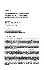
Figure 1.1. An example showing the application of CSAGA with P = 3 to solve a discretized version of G1 [11] (Nopt P  2000).

Based on our previous work, our goal in this chapter is to develop an eective framework that uni es SA, GA, and greedy search for nding CGMdn . In particular, we propose constrained genetic algorithm (CGA) and combined constrained SA and GA (CSAGA) that look for SPdn . We also study algorithms with the optimal average completion time for nding a CGMdn. The algorithms studied in this chapter are all stochastic searches that probe a search space in a random order, where a probe is a neighboring point examined by an algorithm, independent of whether it is accepted or not. Assuming pj to be the probability that an algorithm nds a CGMdn in its j th probe and a simplistic assumption that all probes are independent, the performance of one run of such an algorithm can be characterized by N , the number of probes made (or CPU time taken), and PR (N ), the reachability probability that a CGMdn is hit in any of the N probes:

PR (N ) = 1 ?

N Y j =1

(1 ? pj ); where N  0:

(1.2)

Reachability can be maintained by reporting the best solution found by the algorithm when it stops. As an example, Figure 1.1a plots PR (Ng P ) when CSAGA (see Section 3.2) was run under various number of generations Ng and xed population size P = 3 (where N = Ng P ). The graph shows that PR (Ng P ) approaches one asymptotically as Ng P is increased. Although it is hard to estimate the value of PR (N ) when a test problem is solved by an algorithm, we can always improve the chance of nding a solution by running the same algorithm multiple times, each with N probes, from random starting points. Given PR (N ) for one run of the algorithm and that all runs are independent, the expected total number of probes to nd a CGMdn is: 1 X j =1

PR (N )(1 ? PR (N ))j?1 N  j = P N(N ) : R

(1.3)

Figure 1.1b plots (1.3) based on PR (Ng P ) in Figure 1.1a. In general, there exists Nopt that minimizes (1.3) because PR (0) = 0, limN !1 PR (N ) = 1, PRN(N ) is bounded below by zero, and N PR (N ) ! 1 as N ! 1. The curve in Figure 1.1b illustrates this behavior.

4 Based on the existence of Nopt , we present in Section 3.3 search strategies in CGA and in CSAGA that minimize (1.3) in nding a CGMdn . Finally, Section 4 compares the performance of our algorithms.

2.

Previous Work

In this section, we rst summarize the theory of Lagrange multipliers applied to solve (1.1) and two algorithms developed based on the theory. We then describe existing work in GA for solving constrained NLPs.

2.1.

Theory of Lagrange multipliers for solving discrete constrained NLPs

De ne a discrete equality-constrained NLP as follows [14, 16]: min f (x) x is a vector of bounded (1.4) x subject to h(x) = 0 discrete variables, A generalized discrete augmented Lagrangian function of (1.4) is de ned as follows [14]: (1.5) Ld (x; ) = f (x) + T H (h(x)) + 21 jjh(x)jj2 ; where H is a non-negative continuous transformation function satisfying H (y)  0, H (y) = 0 i y = 0, and  = [1 ;


; m ]T is a vector of Lagrange multipliers. Function H is easy to design; examples include H (h(x)) = [jh1 (x)j;


; jhm (x)j]T and H (h(x)) = [max(h1 (x); 0);


; max(hm (x); 0)]T . Note that these transformations are not used in Lagrangemultiplier methods in continuous space because they are not dierentiable at H (h(x)) = 0. However, they do not pose problems here because we do not require their dierentiability. Similar transformations can be used to transform inequality constraint gj (x)  0 into equivalent equality constraint max(gj (x); 0) = 0. Hence, we only consider problems with equality constraints from here on. We de ne a discrete-neighborhood saddle point SPdn (x ;  ) with the following property: Ld (x ; )  Ld (x ;  )  Ld (x;  ) (1.6) for all x 2 Ndn (x ) and all ; 0 2 Rm . Note that although we use similar terminologies as in continuous space, SPdn is dierent from SPcn (saddle point in continuous space) because they are de ned using dierent neighborhoods. The concept of SPdn is very important in discrete problems because, starting from them, we can derive rst-order necessary and sucient condition for CLMdn that leads to global minimization procedures. This is stated formally in the following theorem [14]: Theorem 1 First-order necessary and sucient condition on CLMdn. [14] A point in the discrete search space of (1.4) is a CLMdn i it satis es (1.6) for any    . Theorem 1 is stronger than its continuous counterparts. The rst-order necessary conditions in continuous Lagrange-multiplier theory [9] require CLMcn to be regular points and functions to be dierentiable. In contrast, there are no such requirements for CLMdn . Further, the rst-order conditions in continuous theory [9] are only necessary, and second-order sucient condition must be checked in order to ensure that a point is actually a CLMcn (CLM in continuous space). In contrast, the condition in Theorem 1 is necessary as well as sucient.

Constrained Genetic Algorithms and their Applications in Nonlinear Constrained Optimization3 1. 2. 3. 4. 5. 6. 7. 8.

procedure CSA (; N ) set initial x [x ;


; xn ;  ;


; k ]T with random x,  0; while stopping0 condition is not satis ed do generate x 2 Ndn (x) using G(x; x0 ); accept x0 with probability AT (x; x0 ) reduce temperature by T T ; end while end procedure

repeat for i 1 to K do call CSA(; N ); end for; increase cooling schedule N N ; until feasible solution has been found and no better solution in two successive increases of N ; 8. end procedure

a) CSA called with schedule N and rate 

b) CSAID : CSA with iterative deepening

1

Figure 1.2.

2.2.

1

1. 2. 3. 4. 5. 6. 7.

5

procedure CSAID

set initial cooling rate  0 and N N0 ; set K number of CSA runs at xed ;

Constrained simulated annealing algorithm (CSA) and its iterative-deepening extension

Existing algorithms for nding SPdn

Since there is a one-to-one correspondence between CGMdn and SPdn , it implies that a strategy looking for SPdn with the minimum objective value will result in CGMdn. We review two methods to look for SPdn . The rst algorithm is the discrete Lagrangian method (DLM) [15]. It is an iterative local search that looks for SPdn by updating the variables in x in order to perform descents of Ld in the x subspace, while occasionally updating the  variables of unsatis ed constraints in order to perform ascents in the  subspace and to force the violated constraints into satisfaction. When no new probes can be generated in both the x and  subspaces, the algorithm has additional mechanisms to escape from such local traps. It can be shown that the point where DLM stops is a CLMdn when the number of neighborhood points is small enough to be enumerated in each descent in the x subspace [14, 16]. However, when the number of neighborhood points is very large and hill-climbing is used to nd the rst point with an improved Ld in each descent, then the point where DLM stops may be a feasible point but not necessarily a SPdn . The second algorithm is the constrained simulated annealing (CSA) [13] algorithm shown in Figure 1.2a. It looks for SPdn by probabilistic descents in the x subspace and by probabilistic ascents in the  subspace, with an acceptance probability governed by the Metropolis probability. Similar to DLM, if the neighborhood of every point is very large and cannot be enumerated, then the point where CSA stops may only be a feasible point but not necessarily a SPdn . Using G(x; x0 ) for generating trial point x0 in Ndn (x), AT (x; x0 ) as the Metropolis acceptance probability, and a logarithmic cooling schedule, CSA has been proven to have asymptotic convergence with probability one to CGMdn [13]. This property is stated in the following theorem: Theorem 2 Asymptotic convergence of CSA. [13] The Markov chain modeling CSA converges to a CGMdn with probability one. Theorem 2 extends a similar theorem for SA that proves its asymptotic convergence to unconstrained global minima of unconstrained optimization problems. By looking for SPdn in the Lagrangian-function space, Theorem 2 shows the asymptotic convergence of CSA to CGMdn in constrained optimization problems. Theorem 2 implies that CSA is not a practical algorithm when used to nd CGMdn in one run with certainty because CSA will take in nite time. In practice, when CSA is run once using a a nite cooling schedule N , it nds a CGMdn with reachability probability PR (N ) < 1. To increase its success probability, CSA with a nite N can be run multiple times from random starting points. Assuming that all the runs are independent, a CGMdn can be found in nite average time de ned by (1.3).

6 success

fail

fail

fail

fail

N PR (N ;Q)

Nopt

t Figure 1.3.

2t 4t 8t 16t

Total time for iterative deepening = 31t Optimal time = 12t

log2 (N )

An application of iterative deepening in CSAID .

We have veri ed experimentally that the expected time de ned in (1.3) has an absolute minimum at Nopt . (Figure 1.1b illustrates the existence of Nopt for CSAGA.) It follows that, in order to minimize (1.3), CSA should be run multiple times from random starting points using schedule Nopt . To nd Nopt at run time without using problem-dependent information, we have proposed to use iterative deepening [7] by starting CSA with a short schedule and by doubling the schedule each time the current run fails to nd a CGMdn [12]. Since the total overhead in iterative deepening is dominated by that of the last run, CSAID (CSA with iterative deepening in Figure 1.2b) has a completion time of the same order of magnitude as that using Nopt when the last schedule that CSA is run is close to Nopt and that this run succeeds. Figure 1.3 illustrates that the total time incurred by CSAID is of the same order as the expected overhead at Nopt . Note that PR (Nopt ) < 1 for one run of CSA at Nopt . When CSA is run with a schedule close to Nopt and fails to nd a solution, its cooling schedule will be doubled and overshoots beyond Nopt . To reduce the chance of overshooting into exceedingly long cooling schedules and to increase the success probability before its schedule reaches Nopt , we have proposed to run CSA multiple times from random starting points at each schedule in CSAID . Figure 1.2b shows CSA that is run K = 3 times at each schedule before the schedule is doubled. Our results show that such a strategy generally requires twice the average completion time with respect to multiple runs of CSA using Nopt before it nds a CGMdn [12].

2.3.

Genetic algorithms for solving constrained NLP problems

Genetic algorithm (GA) is a general stochastic optimization algorithm that maintains a population of alternative candidates and that probes a search space using genetic operators, such as crossovers and mutations, in order to nd better candidates. The original GA was developed for solving unconstrained problems, using a single tness function to rank candidates. Recently, many variants of GA have been developed for solving constrained NLPs. Most of these methods were based on penalty formulations that use GA to minimize an unconstrained penalty function F (x), consisting of a sum of the objective and the constraints weighted by penalties. Similar to CSA, these methods do not require the dierentiability or continuity of functions.

Constrained Genetic Algorithms and their Applications in Nonlinear Constrained Optimization4

7

One penalty formulation is the static-penalty formulation in which all penalties are xed [2]:

F (x; ) = f (x) +

m X i=1

i jhi (x)j ;

(1.7)

where  > 0, and penalty vector = f 1 ; 2 ;


; m g is xed and chosen to be large enough so that F(x ; ) < F (x; ) 8x 2 X ? Xopt and x 2 Xopt : (1.8) Based on (1.8), an unconstrained global minimum of (1.7) over x is a CGMdn to (1.4); hence, it suces to minimize (1.7) in solving (1.4). Since both f (x) and jhi (x)j are lower bounded and x takes nite discrete values, always exists and is nite, thereby ensuring the correctness of the approach. Note that other forms of penalty formulations have also been studied in the literature. The major issue of static-penalty methods lies in the diculty of selecting a suitable . If is much larger than necessary, then the terrain will be too rugged to be searched eectively by local-search methods. If it is too small, then feasible solutions to (1.7) may be dicult to nd. Dynamic-penalty methods [6], on the other hand, address the diculties of static-penalty methods by increasing penalties gradually in the following tness function: m X  F (x) = f (x) + (C  t) jhi(x)j ; j =1

(1.9)

where t is the generation number, and C , , and are constants. In contrast to static-penalty methods, (C  t) , the penalty on infeasible points, is increased during evolution. Dynamic-penalty methods do not always guarantee convergence to CLMdn or CGMdn. For example, consider a problem with two constraints h1 (x) = 0 and h2 (x) = 0. Assuming that a search is stuck at an infeasible point x0 and that for all x 2 Ndn (x0 ), 0 < jh1 (x0 )j < jh1 (x)j, jh2 (x0 )j > jh2 (x)j > 0, and jh1 (x0)j + jh2 (x0)j < jh1 (x)j + jh2 (x)j , then the search can never escape from x0 no matter how large (C  t) grows. One way to ensure the convergence of dynamic-penalty methods is to use a dierent penalty for each constraint, as in Lagrangian formulation (1.5). In the previous example, the search can escape from x0 after assigning a much larger penalty to h2 (x0 ) than that to h1 (x0 ). There are many other variants of penalty methods, such as annealing penalties, adaptive penalties [11] and self-adapting weights [4]. In addition, problem-dependent operators have been studied in the GA community for handling constraints. These include methods based on preserving feasibility with specialized genetic operators, methods searching along boundaries of feasible regions, methods based on decoders, repair of infeasible solutions, co-evolutionary methods, and strategic oscillation. However, most methods require domain-speci c knowledge or problem-dependent genetic operators, and have diculties in nding feasible regions or in maintaining feasibility for nonlinear constraints. In general, local minima of penalty functions are only necessary but not sucient to be constrained local minima of the original constrained optimization problems, unless the penalties are chosen properly. Hence, nding local minima of a penalty function does not necessarily solve the original constrained optimization problem.

3.

A General Framework to look for SPdn

Although there are many methods for solving constrained NLPs, our survey in the last section shows a lack of a general framework that uni es these mechanisms. Without such a framework, it is

8 Generate random initial candidate with initial 

Insert candidate(s) into list based on sorting criterion (annealing or deterministic)

Search in  subspace? x loop

start

Generate new candidates in the x subspace (genetic, probabilistic, or greedy)

N

N

Stopping conditions met?

Y

Generate new candidate(s) in the  subsubace (probabilistic or greedy)

 loop

Update Lagrangian values of all candidates in list (annealing or determinisic)

Y stop Figure 1.4.

An iterative stochastic procedural framework to look for SPdn .

dicult to know whether dierent algorithms are actually variations of each other. In this section we present a framework for solving constrained NLPs that uni es SA, GA, and greedy searches. Based on the necessary and sucient condition in Theorem 1, Figure 1.4 depicts a stochastic procedure to look for SPdn . The procedure consists of two loops: the x loop that updates the variables in x in order to perform descents of Ld in the x subspace, and the  loop that updates the  variables of unsatis ed constraints for any candidate in the list in order to perform ascents in the  subspace. The procedure quits when no new probes can be generated in both the x and  subspaces. The procedure will not stop until it nds a feasible point because it will generate new probes in the  subspace when there are unsatis ed constraints. Further, if the procedure always nds a descent direction at x by enumerating all points in Ndn (x), then the point where the procedure stops must be a feasible local minimum in the x subspace of Ld (x; ), or equivalently, a CLMdn. Both DLM and CSA discussed in Section 2.2 t into this framework, each maintaining a list of one candidate at any time. DLM entails greedy searches in the x and  subspaces, deterministic insertions into the list of candidates, and deterministic acceptance of candidates until all constraints are satis ed. On the other hand, CSA generates new probes randomly in one of the x or  variables, accepts them based on the Metropolis probability if Ld increases along the x dimension and decreases along the  dimension, and stops updating  when all constraints are satis ed. In this section, we use genetic operators to generate probes and present in Section 3.1 CGA and in Section 3.2 CSAGA. Finally, we propose in Section 3.3 iterative-deepening versions of these algorithms.

3.1.

Constrained genetic algorithm (CGA)

CGA in Figure 1.5a was developed based on the general framework in Figure 1.4. Similar to traditional GA, it organizes a search into a number of generations, each involving a population of candidate points in a search space. However, it searches in the Ld space using genetic operators to generate probes in the x subspace, either greedy or probabilistic mechanisms to generate probes in the  subspace, and deterministic organization of candidates according to their Ld values. Lines 2-3 initialize to zero the generation number t and the vector of Lagrange multipliers . The initial population P (t) can be either randomly generated or user provided. Lines 4 and 12 terminate CGA when the maximum number of allowed generations is exceeded. Line 5 evaluates in generation t all candidates in P (t) using Ld (x; (t)) as the tness function.

Constrained Genetic Algorithms and their Applications in Nonlinear Constrained Optimization5 1. procedure CGA(P , Ng ) 2. set generation number t 0 and (t) 0; 3. initialize population P (t); 4. repeat /* over multiple generations */ 5. evaluate Ld (x; (t)) for all candidates in P (t); 6. repeat /* over probes in x subspace */ 7. y GA(select(P (t))); 8. evaluate Ld (y; ) and insert into P (t) 9. until sucient probes in x subspace; 10. (t) (t)  cH(h; P (t)); /* update  */ 11. t t + 1; 12. until (t > Ng ) 13. end procedure a) CGA called with population size P and number of generations Ng . Figure 1.5.

1. 2. 3. 3. 4. 5. 6.

procedure CGAID

7.

end procedure

9

set initial number of generations Ng = N0 ; set K = number of CGA runs at xed Ng ; repeat /* iterative deepening to nd CGMdn */ for i 1 to K do call CGA(P; Ng ) end for set Ng Ng (typically  = 2); until Ng exceeds maximum allowed or (no better solution has been found in two successive increases of Ng and Ng > 5 N0 and a feasible solution has been found);

b) CGAID : CGA with iterative deepening

Constrained GA and its iterative deepening version.

Lines 6-9 explore the x subspace by selecting from P (t) candidates to reproduce using genetic operators and by inserting the new candidates generated into P (t) according to their tness values. After a number of descents in the x subspace (de ned by the number of probes in Line 9 and the decision box \search in  subspace?" in Figure 1.4), the algorithm switches to searching in the  subspace. Line 10 updates  according to the vector of maximum violations H(h(x); P (t)), where the maximum violation of a constraint is evaluated over all the candidates in P (t). That is,

Hi(h(x); P (t)) = xmax H (hi (x)); i = 1;


; m; 2P (t)

(1.10)

where hi (x) is the ith constraint function, H is the non-negative transformation de ned in (1.5), and c is a step-wise constant controlling how fast  changes. Operator  in Figure 1.5a can be implemented in two ways in order to generate a new . A new  can be generated probabilistically based a uniform distribution in ( ?c2H ; c2H ], or in a greedy fashion based on a uniform distribution in (0; cH]. In addition, we can accept new probes deterministically by rejecting negative ones, or probabilistically using an annealing rule. In all cases, a Lagrange multiplier will not be changed if its corresponding constraint is satis ed.

3.2.

Combined Constrained SA and GA (CSAGA)

Based on the general framework in Figure 1.4, we design CSAGA by integrating CSA in Figure 1.2a and CGA in Figure 1.5a into a combined procedure. The new procedure diers from the original CSA in two respects. First, by maintaining multiple candidates in a population, we need to decide how CSA should be applied to the multiple candidates in a population. Our evaluations show that, instead of running CSA corresponding to a candidate from a random starting point, it is best to run CSA sequentially, using the best solution point found in one run as the starting point of the next run. Second, we need to determine the duration of each run of CSA. This is controlled by parameter q that was set to be N6g after experimental evaluations. The new algorithm shown in Figure 1.6 uses both SA and GA to generate new probes in the x subspace. Line 2 initializes P (0). Unlike CGA, any candidate x = [x1 ;


; xn ; 1 ;


; k ]T in P (t) is de ned in the joint x and  subspaces. Initially, x can be user-provided or randomly generated, and  is set to zero.

10 1. procedure CSAGA(P; Ng ) 2. set t 0, T0 , 0 <  < 1, and P (t); 3. repeat /* over multiple generations */ 4. for i 1 to q do /* SA in Lines 5-10 */ 5. for j 1 to P0 do 6. generate xj from Ndn (x ) using G(x ; x0 ); 7. accept x0 with probability AT (x ; x0 ) 8. end for 9. set T ? T ; /* set T for the SA part */ 10. end for 11. repeat /* by GA over probes in x subspace */ 12. y GA(select(P (t))); 13. evaluate Ld (y; ) and insert y into P (t); 14. until sucient number of probes in x subspace; 15. t t + q; /* update generation number */ 16. until (t  Ng ) 17. end procedure j

j

Figure 1.6.

j

j

j

j

CSAGA: Combined CSA and CGA called with population size P and Ng generations.

Lines 4-10 perform CSA using q probes on every candidate in the population. In each probe, we generate probabilistically x0 and accept it based on the Metropolis probability. Experimentally, we set q to be N6g . As discussed earlier, we use the best point of one run as the starting point of the next run. Lines 11-15 start a GA search after the SA part has been completed. The algorithm searches in the x subspace by generating probes using GA operators, sorting all candidates according to their tness values Ld after each probe is generated. In ordering candidates, since each candidate has its own vector of Lagrange multipliers, the algorithm rst computes the average value of Lagrange multipliers for each constraint over all candidates in P (t) and then calculates Ld for each candidate using the average Lagrange multipliers. Note that CSAGA has diculties similar to those of CGA in determining a proper number of candidates to use in its population and the duration of each run. We address these two issues in the CSAGAID in the next subsection. j

3.3.

CGA and CSAGA with iterative deepening

In this section we present a method to determine the optimal number of generations in one run of CGA and CSAGA in order to nd a CGMdn . The method is based on the use of iterative deepening [7] that determines an upper bound on Ng in order to minimize the expected total overhead in (1.3), where Ng is the number of generations in one run of CGA. The number of probes expended in one run of CGA or CSAGA is N = Ng P , where P is the population size. For a xed P , let P^R (Ng ) = PR (PNg ) be the reachability probability of nding CGMdn. From (1.3), the expected total number of probes using multiple runs of either CGA or CSAGA and xed P is:

N = Ng P = P Ng PR (N ) PR (Ng P ) P^R (Ng )

(1.11)

In order to have an optimal number of generations Ngopt that minimizes (1.11), P^RN(Ng g ) must have an absolute minimum in (0,1). This condition is true since P^R (Ng ) of CGA has similar behavior

Constrained Genetic Algorithms and their Applications in Nonlinear Constrained Optimization6

11

as PR (Ng ) of CSA. It has been veri ed based on statistics collected on P^R (Ng ) and Ng at various P when CGA and CSAGA are used to solve ten discretized benchmark problems G1-G10 [11]. Figure 1.1b illustrates the existence of such an absolute minimum when CSAGA with P = 3 was applied to solve G1. Similar to the design of CSAID , we apply iterative deepening to estimate Ngopt . CGAID in Figure 1.5b uses a set of geometrically increasing Ng to nd a CGMdn :

Ngi = i N0 ;

i = 0; 1; : : :

(1.12)

where N0 is the (small) initial number of generations. Under each Ng , CGA is run for a maximum of K times but stops immediately when a feasible solution has been found, when no better solution has been found in two successive generations, and after the number of iterations has been increased geometrically at least ve times. These conditions are used to ensure that iterative deepening has been applied adequately. For iterative deepening to work,  > 1. Let P^R (Ngi ) be the reachability probability of one run of CGA under Ngi generations, Bopt (f 0 ) be the expected total number of probes taken by CGA with Ngopt to nd a CGMdn, and BID (f 0 ) be the expected total number of probes taken by CGAID in Figure 1.5b to nd a solution of quality f 0 starting from N0 generations. According to (1.11),

N Bopt (f 0) = P ^ gopt PR (Ngopt )

(1.13)

The following theorem shows the sucient conditions in order for BID (f 0 ) = O(Bopt (f 0 )). Theorem 3 Optimality of CGAID and CSAGAID . BID (f 0) = O(Bopt(f 0)) if a) P^R (0) = 0; P^R (Ng ) is monotonically non-decreasing for Ng in (0; 1); and limNg !1 P^R (Ng )  1; b) (1 ? P^R (Ngopt ))K  < 1. The proof is not shown due to space limitations. Typically,  = 2, and P^R (Ngopt )  0:25 in all the benchmarks tested. Substituting these values into condition (b) in Theorem 3 yields K > 2:4. In our experiments, we have used K = 3. Since CGA is run a maximum of three times under each Ng , Bopt(f 0 ) is of the same order of magnitude as one run of CGA with Ngopt . The only remaining issue left in the design of CGAID and CSAGAID is in choosing a suitable population size P in each generation. In designing CGAID , we found that the optimal P ranges from 4 to 40 and is dicult to determine a priori. Although it is possible to choose a suitable P dynamically, we do not present the algorithm here due to space limitations and because it performs worse than CSAGAID . In selecting P for CSAGAID , we note in the design of CSAID in Figure 1.2b that K = 3 parallel runs are made at each cooling schedule in order to increase the success probability of nding a solution. For this reason, we set P = K = 3 in our experiments. Our experimental results in the next section show that, although the optimal P may be slightly dierent from 3, the corresponding expected overhead to nd a CGMdn diers very little from that when a constant P is used.

12

4.

Experimental Results

We present in this section our experimental results in evaluating CSAID , CGAID and CSAGAID on discrete constrained NLPs. Based on the framework in Figure 1.4, we rst determine the best combination of strategies to use in generating probes and in organizing candidates. Using the best combination of strategies, we then show experimental results on some constrained NLPs. Due to a lack of large-scale discrete benchmarks, we derive our benchmarks from two sets of continuous benchmarks: Problem G1-G10 [11, 8] and Floudas and Pardalos' Problems [5].

4.1.

Implementation Details

In theory, algorithms derived from the framework, such as CSA, CGA, and CSAGA, will look for SPdn . In practice, however, it is important to choose appropriate neighborhoods and generate proper trial points in x and  subspaces in order to solve constrained NLPs eciently. An important component of these methods is the frequency at which  is updated. Like in CSA [13], we have set experimentally in CGA and CSAGA the ratio of generating trial points in x and  subspaces from the current point to be 20n to m, where n is the number of variables and m is the number of constraints. This ratio means that x is updated more often than . In generating trial points in the x subspace, we have used a dynamically controlled neighborhood size in the SA part [13] based on the 1:1 ratio rule [3], whereas in the GA part, we have used the seven operators in Genocop III [10] and Ld as our tness function. In implementing CSAID , CGAID and CSAGAID , we have used the default parameters of CSA [13] in the SA part and those of Genocop III [10] in the GA part. The generation of trial point 0 in the  subspace is done by the following rule:

0j = j + r1 j

where j = 1;


; m:

(1.14)

Here, r1 is randomly generated in [?1=2; +1=2] if we choose to generate  probabilistically, and is randomly generated in [0; 1] if we choose to generate probes in  in a greedy fashion. We adjust  adaptively according to the degree of constraint violations, where

 = w H(x) = [w1 H1 (x); w2 H2 (x);


; wm Hm(x)];

(1.15)

represents vector product, and H is the vector of maximum violations de ned in (1.10). When Hi(x) is satis ed, i does not need to be updated; hence, i = 0. In contrast, when a constraint is not satis ed, we adjust i by modifying wi according to how fast Hi (x) is changing:  i (x) > 0 T wi = 0 wwi ifif H (1.16) H 1 i i (x) < 1 T where T is the temperature, and 0 = 1:25, 1 =0.8, 0 = 1:0, and 1 = 0:01 were chosen experimentally. When Hi (x) is reduced too quickly (i.e., Hi (x) < 1 T ), Hi (x) is over-weighted, leading to possibly poor objective values or diculty in satisfying other under-weighted constraints. Hence, we reduce i 's neighborhood. In contrast, if Hi (x) is reduced too slowly (i.e., Hi(x) > 0 T ), we enlarge i 's neighborhood in order to improve its chance of satisfaction. Note that wi is adjusted using T as a reference because constraint violations are expected to decrease when T decreases. In addition, for iterative deepening to work, we have set the following parameters:  = 2, K = 3, N0 = 10
nv , and Nmax = 1:0  108 nv , where nv is the number of variables, and N0 and Nmax are, respectively, initial and maximum number of probes.

Constrained Genetic Algorithms and their Applications in Nonlinear Constrained Optimization7

13

Timing results on evaluating various combinations of strategies in CSAID , CGAID and CSAGAID with P = 3 to nd solutions that deviate by 1% and 10% from the best-known solution of a discretized version of G2. Table 1.1.

All CPU times in seconds were averaged over 10 runs and were collected on a Pentinum III 500-MHz computer with Solaris 7. '?' means that no solution with desired quality can be found. Probe Generation Strategy  subspace x subspace probabilistic probabilistic probabilistic probabilistic probabilistic deterministic probabilistic deterministic greedy probabilistic greedy probabilistic greedy deterministic greedy deterministic

4.2.

Insertion Strategy annealing deterministic annealing deterministic annealing deterministic annealing deterministic

Evaluation Results

Target Solution 1% o CGMdn Target Solution 10% o CGMdn

CSAID CGAID CSAGAID CSAID CGAID CSAGAID 4.89 sec. 1.35 sec. ? 1.03 sec.

6.91 sec. 23.99 sec. 9.02 sec. ? ? 18.76 sec. ? 16.73 sec. 7.02 sec. ? 7.02 sec. ? ? 25.50 sec. ? 25.50 sec.

6.93 sec. 1.35 sec. 2.78 sec. ? 89.21 sec. 2.40 sec. ? ? 2.18 sec. 7.75 sec. 1.36 sec. ? 7.75 sec. 1.36 sec. ? ? 82.24 sec. 1.90 sec. ? 82.24 sec. 1.90 sec.

1.03 sec.

? ?

0.90 sec. 0.90 sec.

? ?

Due to a lack of large-scale discrete benchmarks, we derive our benchmarks from two sets of continuous benchmarks: Problem G1-G10 [11, 8] and Floudas and Pardalos' Problems [5]. In generating a discrete constrained NLP, we discretize continuous variables in the original continuous constrained NLP into discrete variables as follows. In discretizing continuous variable xi in range [li ; ui ], where li and ui are lower and upper bounds of xi , respectively, we force xi to take values from the set: 8n o < ai + bi ?ai j; j = 0; 1;


; s if bi ? ai < 1 (1.17) Ai = :  1 s ai + s j; j = 0; 1;


; b(bi ? ai )sc if bi ? ai  1; where s = 1:0  107 . Table 1.1 shows the results of evaluating various combinations of strategies in CSAID , CGAID , and CSAGAID on a discretized version of G2 [11, 8]. We show the average time of 10 runs for each combination in order to reach two solution quality levels (1% or 10% worse than CGMdn , assuming the value of CGMdn is known). Evaluation results on other benchmark problems are similar and are not shown due to space limitations. Our results show that CGAID is usually less ecient than CSAID or CSAGAID . Further, CSAID or CSAGAID has better performance when probes generated in the x subspace are accepted by annealing rather than by deterministic rules (the former prevents a search from getting stuck in local minima or infeasible points). On the other hand, there is little dierence in performance when new probes generated in the  subspace are accepted by probabilistic or by greedy rules and when new candidates are inserted according to annealing or deterministic rules. In short, generating probes in the x and  subspaces probabilistically and inserting candidates in both the x and  subspaces by annealing rules leads to good and stable performance. For this reason, we use this combination of strategies in our experiments. We next test our algorithms on ten constrained NLPs G1-G10 [11, 8]. These problems have objective functions of various types (linear, quadratic, cubic, polynomial, and nonlinear) and constraints of linear inequalities, nonlinear equalities, and nonlinear inequalities. The number of variables is up to 20, and that of constraints, including simple bounds, is up to 42. The ratio of feasible space with respect to the whole search space varies from 0% to almost 100%, and the topologies of feasible regions are quite dierent. These problems were originally designed to be solved by evolutionary

14 Table 1.2. Results on CSAID , CGAID and CSAGAID in nding the best-known solution f  for 10 discretized constrained NLPs and their corresponding results found by EA. (S.T. stands for strategic oscillation, H.M. for homomorphous mappings, and D.P. for dynamic penalty. BID (f  ), the CPU time in seconds to nd the best-known solution f  , were averaged over 10 runs and were collected on a Pentinum III 500-MHz computer with Solaris 7. #Ld represents the number of Ld (x; )-function evaluations. The best BID (f  ) for each problem is boxed.)

Problem Best ID Solution f  G1 (min) -15 G2 (max) -0.80362 G3 (max) 1.0 G4 (min) -30665.5 G5 (min) 4221.9 G6 (min) -6961.81 G7 (min) 24.3062 G8 (max) 0.095825 G9 (min) 680.63 G10 (min) 7049.33

EAs CSAID CGAID CSAGAID Best Found Method BID (f  ) #Ld Popt BID (f  ) P BID (f  ) #Ld Popt BID (f  ) ? -15 Genocop 1.65 sec. 173959 40 5.49 sec. 3 1.64 sec. ?172435 2 1.31 sec. ?
0.803553 S.T. 7.28 sec. 415940 30 311.98 sec. 3 5.18 sec. ?
261938 3 5.18 sec. ?
1.0 S.T. 1.07 sec. ?123367 30 14.17 sec. 3 0.89 sec.
104568 3 0.89 sec.
-30664.5 H.M. 0.76 sec.
169913 5 3.95 sec. 3 0.95 sec. 224025 3 0.95 sec. ? 5126.498 D.P. 2.88 sec. 506619 30 68.9 sec. 3 2.76 sec. 510729 2 2.08 sec. ?
-6961.81 Genocop 0.99 sec. 356261 4 7.62 sec. 3 0.91 sec. 289748 2 0.73 sec. ?
24.62 H.M. 6.51 sec. 815696 30 31.60 sec. 3 4.60 sec. 547921 4 4.07 sec. ?
0.095825 H.M. 0.11 sec. 21459 30 0.31 sec. 3 0.13 sec. ? 26585 4 0.10 sec. ?
680.64 Genocop 0.74 sec. ?143714 30 5.67 sec. 3 0.57 sec.
110918 3 0.57 sec.
7147.9 H.M. 3.29 sec.
569617 30 82.32 sec. 3 3.36 sec. 608098 3 3.36 sec.

algorithms (EAs) in which constraint handling techniques were tuned for each problem in order to get good results. Examples of such techniques include keeping a search within feasible regions with speci c genetic operators and dynamic and adaptive penalty methods. Table 1.2 compares the performance of CSAID , CGAID , and CSAGAID with respect to BID (f  ), the expected total CPU time of multiple runs until a solution of value f  is found. The rst two columns show the problem IDs and the corresponding known f  . The next two columns show the best solutions obtained by EAs and the speci c constraint handling techniques used to generate the solutions. Since all CSAID , CGAID and CSAGAID can nd a CGMdn in all 10 runs, we compare their performance with respect to T , the average total overhead of multiple runs until a CGMdn is found. The fth and sixth columns show, respectively, the average time and number of Ld (x; ) function evaluations CSAID takes to nd f . The next two columns show the performance of CGAID with respect to Popt , the optimal population size found by enumeration, and the average time to nd f . These results show that CGAID is not competitive as compared to CSAID , even when Popt is used. The results on including additional steps in CGAID to select a suitable P at run time are worse and are not shown due to space limitations. Finally, the last ve columns show the performance of CSAGAID . The rst three present the average times and number of Ld (x; ) evaluations using a constant P , whereas the last two show the average times using Popt found by enumeration. These results show little improvements in using Popt . Further, CSAGAID has between 9% and 38% in improvement in BID (f  ), when compared to that of CSAID , for the 10 problems except for G4 and G10. Comparing CGAID and CSAGAID with EA, we see that EA was only able to nd f  in three of the ten problems, despite extensive tuning and using problem-speci c heuristics, whereas both CGAID and CSAGAID can nd f  for all these problems without any problem-dependent strategies. It is not possible to report the timing results of EA because the results are the best among many runs after extensive tuning. Finally, Table 1.3 shows the results on selected discretized Floudas and Pardalos' benchmarks [5] that have more than 10 variables and that have many equality or inequality constraints. The rst three columns show the problem IDs, the known f  , and the number of variables (nv ) in each. The

Constrained Genetic Algorithms and their Applications in Nonlinear Constrained Optimization8

15

Table 1.3. Results on CSAID and CSAGAID with P = 3 in solving selected Floudas and Pardalos' discretized constrained NLP benchmarks (with more than nv = 10 variables). Since Problem 5: and 7: are especially large and dicult and a search can rarely reach their true CGMdn , we consider a CGMdn found when the solution quality is within 10% of the true CGMdn . All CPU times in seconds were averaged over 10 runs and were collected on a Pentium-III 500-MHz computer with Solaris 7. Problem f (x) CSAID CSAGAID ID Best f  nv BID (f  )  BID (f  ) ? 2.7.1(min) -394.75 20 35.11 sec. 14.86 sec.
? 2.7.2(min) -884.75 20 53.92 sec. 15.54 sec.
? 2.7.3(min) -8695.0 20 34.22 sec. 22.52 sec.
? 2.7.4(min) -754.75 20 36.70 sec. 16.20 sec.
? 2.7.5(min) -4150.4 20 89.15 sec. 23.46 sec.
? 5.2(min) 1.567 46 3168.29 sec. 408.69 sec.
? 5.4(min) 1.86 32 2629.52 sec. 100.66 sec.
? 7.2(min) 1.0 16 824.45 sec. 368.72 sec.
? 7.3(min) 1.0 27 2323.44 sec. 1785.14 sec. ?
7.4(min) 1.0 38 951.33 sec. 487.13 sec.


last two columns compare BID (f  ) of CSAID and CSAGAID with xed P = 3. They show that CSAGAID is consistently faster than CSAID (between 1.3 and 26.3 times), especially for large problems. This is attributed to the fact that GA maintains more diversity of candidates by keeping a population, thereby allowing competition among the candidates and leading SA to explore more promising regions.

5.

Conclusions

In this chapter we have presented new algorithms to look for discrete-neighborhood saddle points in discrete Lagrangian space of constrained optimization problems. Our results show that genetic algorithms, when combined with simulated annealing, are eective in locating saddle points. Future developments will focus on better ways to select appropriate heuristics in probe generation, including search direction control and neighborhood size control, at run time.

References

[1] E. Aarts and J. Korst. Simulated Annealing and Boltzmann Machines. J. Wiley and Sons, 1989. [2] D. P. Bertsekas. Constrained Optimization and Lagrange Multiplier Methods. Academic Press, 1982. [3] A. Corana, M. Marchesi, C. Martini, and S. Ridella. Minimizing multimodal functions of continuous variables with the simulated annealing algorithm. ACM Trans. on Mathematical Software, 13(3):262{280, 1987. [4] A.E. Eiben and Zs. Ruttkay. Self-adaptivity for constraint satisfaction: Learning penalty functions. Proceedings of the 3rd IEEE Conference on Evolutionary Computation, pages 258{ 261, 1996. [5] C. A. Floudas and P. M. Pardalos. A Collection of Test Problems for Constrained Global Optimization Algorithms, volume 455 of Lecture Notes in Computer Science. Springer-Verlag, 1990. [6] J. Joines and C. Houck. On the use of non-stationary penalty functions to solve nonlinear constrained optimization problems with gas. Proceedings of the First IEEE International Conference on Evolutionary Computation, pages 579{584, 1994. [7] R. E. Korf. Depth- rst iterative deepening: An optimal admissible tree search. Arti cial Intelligence, 27:97{109, 1985. [8] S. Koziel and Z. Michalewicz. Evolutionary algorithms, homomorphous mappings, and constrained parameter optimization. Evolutionary Computation, 7(1):19{44, 1999. [9] D. G. Luenberger. Linear and Nonlinear Programming. Addison-Wesley Publishing Company, Reading, MA, 1984. [10] Z. Michalewicz and G. Nazhiyath. Genocop III: A co-evolutionary algorithm for numerical optimization problems with nonlinear constraints. Proceedings of IEEE International Conference on Evolutionary Computation, 2:647{651, 1995. [11] Z. Michalewicz and M. Schoenauer. Evolutionary algorithms for constrained parameter optimization problems. Evolutionary Computation, 4(1):1{32, 1996. [12] B. W. Wah and Y. X. Chen. Optimal anytime constrained simulated annealing for constrained global optimization. Sixth Int'l Conf. on Principles and Practice of Constraint Programming, September 2000. 17

18 [13] B. W. Wah and T. Wang. Simulated annealing with asymptotic convergence for nonlinear constrained global optimization. Principles and Practice of Constraint Programming, pages 461{475, October 1999. [14] B. W. Wah and Z. Wu. The theory of discrete Lagrange multipliers for nonlinear discrete optimization. Principles and Practice of Constraint Programming, pages 28{42, October 1999. [15] Z. Wu. Discrete Lagrangian Methods for Solving Nonlinear Discrete Constrained Optimization Problems. M.Sc. Thesis, Dept. of Computer Science, Univ. of Illinois, Urbana, IL, May 1998. [16] Z. Wu. The Theory and Applications of Nonlinear Constrained Optimization using Lagrange Multipliers. Ph.D. Thesis, Dept. of Computer Science, Univ. of Illinois, Urbana, IL, October 2000.