Constraint-Based Dynamic Programming for ... - CiteSeerX

Constraint-Based Dynamic Programming for Decentralized POMDPs with Structured Interactions Akshat Kumar and Shlomo Zilberstein Department of Computer Science University of Massachusetts Amherst, MA, 01003

{akshat, shlomo}@cs.umass.edu ABSTRACT

broadcast channel protocols [2], and target tracking in sensor networks [8] can be formulated as DEC-POMDPs. Solving DEC-POMDPs optimally is NEXP-hard [2], with optimal algorithms able to provide solution for very small problems involving two agents and small horizons [6, 17]. Approximate algorithms can scale up the horizon, but they remain limited to a few agents [14, 3]. An emerging approach to improve scalability has been to consider restricted forms of interaction that arise frequently in practice [1, 11]. In particular, ND-POMDP [11] is one such general model which is inspired by a realistic sensor network coordination problem [8]. The key assumption in ND-POMDP is that of transition and observation independence and the locality of interaction, which help construct efficient algorithms that exploit the independence among the agents. A rich portfolio of algorithms has been developed for solving ND-POMDPs, featuring locally optimal policy search [11], approximation schemes [18, 10] and a globally optimal algorithm [11]. Most of these algorithms are based on policy search. To the best of our knowledge, no bottom up dynamic programming (DP) algorithm exists. The advantage of the DP approach lies in its ability to focus planning on the reachable part of the belief space using a forward heuristic search. Such approximate DP algorithms–often referred to as pointbased dynamic programming techniques–have shown great success in solving POMDPs. The algorithm we introduce, Constraint-Based Dynamic Programing (CBDP), shares its motivation with such point-based approaches. The efficiency of CBDP lies in effectively capturing the independence and structure among agents using constraints. CBDP uses a factored MDP-based heuristic function to identify relevant belief points. Solving a factored MDP is not easy, as the space of both the joint actions and states is exponential in the number of agents. We provide a novel way to approximate this value function efficiently using constraint optimization. The planning (backup operation in DP) for these beliefs is performed using a constraint-based formulation rather than a naive search through the exponential number of policies. Such formulation makes the complexity of CBDP exponential only in the induced width of the depthfirst search (DFS) ordering of the agent interaction graph, while linear in the number of agents. This enhances the scalability of CBDP for our sensor network domain, allowing us to solve large loosely-coupled multi-agent planning problems. Our results show that CBDP can handle very large domains. It can solve efficiently problems with hundreds of horizon steps while providing orders of magnitude time savings over the previous best algorithm.

Decentralized partially observable MDPs (DEC-POMDPs) provide a rich framework for modeling decision making by a team of agents. Despite rapid progress in this area, the limited scalability of solution techniques has restricted the applicability of the model. To overcome this computational barrier, research has focused on restricted classes of DECPOMDPs, which are easier to solve yet rich enough to capture many practical problems. We present CBDP, an efficient and scalable point-based dynamic programming algorithm for one such model called ND-POMDP (Network Distributed POMDP). Specifically, CBDP provides magnitudes of speedup in the policy computation and generates better quality solution for all test instances. It has linear complexity in the number of agents and horizon length. Furthermore, the complexity per horizon for the examined class of problems is exponential only in a small parameter that depends upon the interaction among the agents, achieving significant scalability for large, loosely coupled multi-agent systems. The efficiency of CBDP lies in exploiting the structure of interactions using constraint networks. These results extend significantly the effectiveness of decision-theoretic planning in multi-agent settings.

Categories and Subject Descriptors I.2 [Artificial Intelligence]: [Dynamic programming, Multiagent systems, Intelligent agents]

Keywords Multiagent planning, DEC-POMDPs

1.

INTRODUCTION

DEC-POMDPs have emerged in recent years as an important framework for modeling team decision problems under uncertainty. They can effectively capture situations when the environment state dynamics and the reward system depend upon the joint action of all agents, but agents must act based on different partial knowledge of the overall situation. Many problems such as multi-robot coordination [14], Cite as: Constraint-Based Dynamic Programming for Decentralized Cite as: with Constraint-Based Dynamic Akshat Programming for Decentralized POMDPs Structured Interactions, Kumar, Shlomo Zilberstein,

POMDPs with Int. Structured Akshat Kumar, ZilberProc. of 8th Conf.Interactions, on Autonomous AgentsShlomo and Multiastein, Systems Proc. of 8th Int. Conf. on Autonomous andSierra Multiagent Sysgent (AAMAS 2009) , Decker,Agents Sichman, and Castel-

tems (AAMAS 2009), Decker, Sichman, Sierra and Castelfranchi (eds.), franchi (eds.), May, 10–15, 2009, Budapest, Hungary, pp. XXX-XXX. May, 10–15, Hungary, pp. 561–568 c 2009, Copyright 2009, Budapest, International Foundation for Autonomous Agents and Multiagent Systems All rights reserved. Agents Copyright © 2009, (www.ifaamas.org). International Foundation for Autonomous and Multiagent Systems (www.ifaamas.org), All rights reserved.

561

AAMAS 2009 • 8th International Conference on Autonomous Agents and Multiagent Systems • 10–15 May, 2009 • Budapest, Hungary

W

N S 1

E

loc1

W

N S 2

E

loc2

W

N S 3

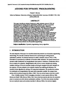
R R(s, a) = Σl Rl (sl , su , al ). The reward function is decomposable among sub groups of agents referred by l. If k agents i1 , . . . , ik are involved in a particular sub group l, then sl denotes the state along the link i.e. si1 , . . . , sik . Similarly, al = ai1 , . . . , aik . In the sensor domain in Figure 1, the reward is decomposed among two subgroups (sensor 1–sensor 2) and (sensor 2–sensor 3), hence R = R12 (s1 , s2 , su , a1 , a2 ) + R23 (s2 , s3 , su , a2 , a3 ). Based on the reward function, an interaction hypergraph can be constructed. A hyperlink l connects the subset of agents which form the reward component Rl . This hypergraph visually depicts the dependency among agents and is an important tool for the complexity analysis in later sections.

E

Figure 1: A 3-chain sensor network configuration. Each sensor can scan in 4 directions. Target moves stochastically between loc1 and loc2.

2.

BACKGROUND

This section briefly introduces the motivating sensor network domain and the ND-POMDP model. More details can be found in [8, 11].

2.1

Coordinated target tracking

bo bo = (bu , b1 , . . . , bn ) is the initial belief for joint state s = su , s1 , . . . , sn and b(s) = b(su ) · Πn i=1 b(si ).

Our target application is illustrated in Figure 1, which shows a 3-chain sensor network configuration. Each sensor has scanning ability in four directions (North, South, East, West). The target moves stochastically between loc1 and loc2. To track the target and obtain the associated reward the sensors with the overlapping area must scan the area together. For example, if the target is present in loc1 then sensor 1 must scan East and sensor 2 must scan West to track it. Thus, coordination plays an important role. The movement of targets is unaffected by sensor agents. Sensors have imperfect observability of the target, so there can be false positive and negative observations. On successfully tracking a target, sensors receive a reward. Otherwise they incur a cost, when they scan an area in an uncoordinated fashion or when the target is absent. The specifications of the model are taken from [11].

2.2

Solving the above decision problem requires to compute the joint policy π = π1 , . . . , πn that maximizes the total expected reward of all agents over a finite horizon T starting from the initial belief bo . The following theorem illustrates an important advantage of transition and observation independence in ND-POMDP. Theorem 1. Given transition and observation independence, and a decomposable reward function, the value of a joint policy π is also decomposable. That is, X t t t → → ω t) = Vπl (sl , su , − ω tl ). Vπt (st , − l

Hence, the value function of a policy in ND-POMDP can be represented as a sum of local value functions, one for each link. For proof please refer to [11].

ND-POMDP model

The problem of target tracking in sensor networks can be easily represented as a DEC-POMDP [2]. However, explicit utilization of independence among the agents can help us construct more efficient algorithms. For example, sensors in our domain are mostly independent–their state transitions given the target location and the observations are independent of the actions of the other agents. Agents are coupled only through the joint reward function. The ND-POMDP model [11] can express such independence relations. It is described below for a group of n sensor agents.

3.

S = ×1≤i≤n Si × Su . Si refers to the local state of agent i. Su refers to a set of uncontrollable states that are independent of the actions of the agents. In the sensor network example, Si is empty, while Su corresponds to the set of locations where targets can be present. A = ×1≤i≤n Ai where Ai is the set of actions for agent i. For the sensor network example A1 = {N, W, E, S, Off}. Ω = ×1≤i≤n Ωi is the joint observation set. P P (s |s, a) = Pu (su |su ) · Π1≤i≤n Pi (si |si , su , ai ), where a = a1 , . . . , an is the joint action performed in joint state s = su , s1 , . . . , sn resulting in joint state s = su , s1 , . . . , sn . This relies on transition independence. O O(ω|s, a) = Π1≤i≤n Oi (ωi |si , su , ai ), where s is the joint state resulting after taking joint action a and receiving joint observation ω. This relies on observation independence.

562

POINT-BASED DYNAMIC PROGRAMMING

The intractability of optimal (DEC) POMDP algorithms can be attributed to planning for the complete belief space. DEC-POMDPs are further disadvantaged as the joint policy has to be represented explicitly and cannot be extracted directly from the value function. The idea of planning for a finite set of belief points has been explored by Lovejoy [9], leading to several successful point-based POMDP algorithms such as PBVI [13], Perseus [16], and FSVI [15] among others. For DEC-POMDPs, a similar point-based algorithm called MBDP has been developed by Seuken and Zilberstein [14]. However, extending MBDP to multiple agents (>2) is nontrivial because the computational cost of planning as well as the MDP heuristic will require exponential effort. Even representing the problem parameters (reward, transition function) will be exponential in the number of agents, clearly infeasible. CBDP shares its motivation with these successful point-based algorithms. However, it is significantly different from MBDP as it exploits the structure of interactions in the ND-POMDP, whereas MBDP is oblivious to such structure. Next, we presents several novel techniques we employ in CBDP to enable efficient planning for multiple agents. Algorithm 1 shows the general point-based dynamic programming framework that CBDP follows. The input is a finite horizon problem with T decision steps. The algorithm first computes the heuristic function used for sampling belief points for each time step t. Then, the main bottom-up

Akshat Kumar, Shlomo Zilberstein • Constraint-Based Dynamic Programming for Decentralized POMDPs with Structured Interactions

Algorithm 1: Point-based DP framework 1 2 3 4 5 6 7 8 9

T ← horizon of the problem Belief set B ← {} Precompute the belief selection heuristic →T − Q ← all one step policy trees for t = T − 1 until 1 do →t+1 e t ← DoBackup(− Q ) Q Populate B using heuristic function →t − e t ,B) Q ← findBest(Q →1 − Output Q as the solution

l at time step t when the involved agents perform the action al , i.e. rlt = Rl (stl , stu , al ). Let ptu denote the transition of t the unaffected state at time t, i.e. ptu = P (st+1 u |su ). Let pti denote the transition probability of agent i, i.e. pti = |sti , stu , ai ). Similar shorthand notation can be dePi (st+1 i fined for a link l as well: ptl is the product of the transition probabilities of all the agents (say k) involved in the link l, i.e. ptl = pl1 . . . plk . The context of states and actions will become clear from the usage. The MDP value of any joint state st−1 , V (st−1 ), can be defined as follows: X P (st |st−1 , a)V (st )). V (st−1 ) = max(R(st−1 , a) + a

dynamic programming loop starts. For each step t, the set →t − Q = {qit |1 ≤ i ≤ n} contains the best policies for each agent. The set qit includes policies for agent i that contributed to the best joint policy for some sampled belief. The algorithm starts with the last time step, where there are only immediate actions to take. These actions, which are → − relatively few, are stored in the set Q T without any belief sampling. In each further iteration, the backup of the last e t . Then, a desired number step’s best policies is stored in Q of beliefs are sampled using the precomputed heuristic function. For each of the sampled beliefs, the best joint policy →t e t and stored in − Q , which forms is extracted from the set Q the basis for the next iteration. Finally, at t = 1, the best policy for the initial belief bo is found and returned as the solution. Note that the space and time complexity is defined by the number of sampled beliefs as planning is restricted only to this set. This is the key factor in the efficiency and scalability of point-based approaches. We now examine the main steps of Algorithm 1 as implemented in CBDP: 1) Computation of the heuristic function; 2) Belief sampling using heuristic function; and 3) Finding the best joint policy for a particular belief. Contrary to a single-agent POMDP, each of these steps is non-trivial for multiple agents. First, the well known MDP heuristic for POMDPs translates to a factored MDP, which is difficult to solve due to exponential state and action space [7]. Second, belief sampling requires reasoning about joint states and actions, which again requires exponential effort if done naively. Finally, computing the best joint policy for a given belief could require search through the exponential number of candidates. We show in the following sections how we perform efficiently each one of these steps of CBDP.

3.1

Heuristic function computation

We use as a heuristic the factored MDP derived from the original ND-POMDP model by ignoring the observations. The optimal policy of this MDP is used for belief sampling in CBDP. One would intuitively believe that the factored state and the reward dynamics of this MDP will make the value function structured, making it easier to compute the optimal policy. Unfortunately, this is not the case. The value function eventually depends on all the states as has been shown by Koller and Parr [7]. This makes the policy harder to compute. To address this, we introduce a way to approximate the value function such that it becomes structured and efficiently computable. To simplify the equations, we introduce some shorthand notation. Let rlt denote the immediate reward along the link

st

which can be simplified as follows using the above notation and the transition independence of the factored MDP. X t−1 rl + V (st−1 ) = max( a

X

t−1 t−1 . . . pn V (st )) pt−1 u p1

stu ,st1 ...stn

l

(1) The time complexity of solving Eq. 1 for all horizons is O(T |Ai |n |Su |2 |Si |2n ). The presence of two exponential terms, |Ai |n and |Si |2n , makes it harder to compute. We inductively define an approximate function Vˆ , which is an upper bound on the optimal value function. Vˆ is decomposable along the links and is thus easier to compute. For the last time step T , Vˆ is defined as the sum of immediate rewards for each link. Thus, it is trivially decomposable along the links. Let us assume inductively that for P time step t, Vˆ is decomposable, i.e. Vˆ (st ) = l Vˆlt (stu stl |st ). The conditioning over the current state is necessary as the two different joint states s, s may share the state component su sl along the link l, and the value V (su sl ) may be different in states s and s . For example, let s = su s1 s2 s3 , s = su s1 s2 s4 and the state along a link be s1 s2 . The value V (su s1 s2 ) can be different for s and s although they share the state along the link. The derivation of Vˆ for the previous step t−1 is as follows. Define a new function Vˆ for the step t − 1: X t−1 X t−1 ˆ t rl + pu . . . pt−1 Vˆ (st−1 ) = max{ n V (s )} a

l

st

Clearly, Vˆ (st−1 ) is an upper bound on the exact value V (st−1 ) because we assumed Vˆ (st ) was an upper bound on V (st ). In the following we derive Vˆ from Vˆ X t−1 X t−1 ˆ t Vˆ (st−1 ) = max{ rl + pu . . . pt−1 n V (s )} a

l

st

l

st

X t−1 X t−1 X t t t t Vˆl (su sl |s )} rl + pu . . . pt−1 = max{ n a

X t−1 rl + ≤ max{ a

l

X

l

put−1

stu ,st1 ...stn

t−1 . . . pn

X l

max Vˆlt } st | {z }

The quantity under the brace is uniquely defined for each t of the link l and thus can be replaced with Vel (stu stl ) = t t t t ˆ maxst Vl (su sl |s ). Intuitively, this approximation will perform better when the sensor agents along a link in a particular state (sl ) with a given external state (su ) provide similar contribution to the value function across all joint states (st ). Upon rearranging the terms of the previous equation we

563


are involved. Therefore, coordination graphs can be solved efficiently for large loosely coupled systems.

A1 Q12

Q13

3.1.2

A3

A2 Q24

Q34 A4

Figure 2: A coordination graph for 4 agents get X

X t−1 X rl + = max{ a

l

l

X t−1 X = max{ rl + a

l

l

t pt−1 . . . pt−1 Vel } u n

stu ,st1 ...stn

X

t−1 t−1 e t p−l Vl } pt−1 u pl

stu ,stl ,st−l

slt−1 refers to the state of agents along the link l, st−l refers to the state of the rest of the agents. Similarly, pt−1 −l abbreviates the transition probability product of agents except those on link l. pt−1 −l is independent of the rest of the terms and will sum up to 1. Finally, we obtain the decomposable Vˆ which was our goal. X t−1 X t−1 t−1 t (rl + pu pl Vel ) (2) Vˆ (st−1 ) = max a

3.1.1

l

Complexity

Computing the policy for our factored MDP requires solving Eq. 2 for each state and time step t using coordination graphs. The time complexity is O(nT |Su |2 |Si |2n |Ai |d ) where d is the induced width of the coordination graph. The space complexity is O(T |Su ||Si |n + n|Ai |d ). The term |Ai |d refers to the space requirement of the bucket elimination algorithm. The exponential factor corresponding to the state space still remains. However, note that for the sensor network domain, the internal states are empty. This makes the time complexity O(nT |Su |2 ||Ai |d ) and space complexity O(T |Su | + n|Ai |d ) which are polynomial in the state space and linear in the number of agents. Hence, for the sensor network domain we can effectively solve large problems with low induced width.

3.2

Belief sampling

This section describes the belief sampling for any horizon t. We use a portfolio of three heuristic functions: one based purely on the underlying MDP, another taking observations into account, and finally the random heuristic.

3.2.1

MDP-based sampling

In the pure MDP-based sampling, the underlying joint state is revealed after each step. In POMDPs this is easy as we draw a state from the current belief b. However, in a DEC-POMDP the belief is over joint states, hence one has to reason about the joint state space. But fortunately, in a ND-POMDP, b(s) = bu (su )b1 (s1 ) . . . bn (sn ). This allows us to sample each factored state from its corresponding distribution. Once we get the current underlying joint state st = (stu . . . stn ), we select the action a using the precomputed MDP policy. Then, the next unaffected state is sam= Sample(P (·|stu )). Each pled from the distribution st+1 u t+1 can be sampled as s = Sample(P (·|sti , stu , ai )). state st+1 i i Repeated simulations using such a scheme gives us a belief point for any horizon starting from the initial belief bo .

stu ,stl

Joint action selection

Solving Eq. 2 still requires iterating over exponential number of actions. We now show how it can be solved efficiently for each state st using coordination graphs. These graphs, which were first introduced in the context of factored MDPs [5], are essentially constraint networks whose solution corresponds to the solution of the underlying constraint optimization problem. A coordination graph is very similar to the interaction graph defined using reward functions. There is a node for each agent and an edge (or an hyper-edge) connects nodes for agents that are part of the same reward component Rl . Agents have Q functions defining the local rewards, which also depends upon some other agents–exactly those which share the same reward component. For example, in Figure 2 agent A2 has two Q functions, Q12 shared with agent A1 along the link A1 − A2 and Q24 . Eq. 2 can be solved for every state st by formulating a joint task for the agents to find the joint P action a that maximizes the sum of all Q functions l Ql . The Q function is defined for each link l as follows. X t+1 ptu ptl Vel st : Ql (al ) = rlt +

3.2.2 Direct belief space exploration One shortcoming of the MDP heuristic is that it ignores the effect of observations which are important to determine the belief state accurately in a partially observable environment. To overcome this limitation, Shani et al. proposed a new MDP-based heuristic that directly explores the belief space [15]. Our second heuristic is motivated by this approach, presented in the Algorithm 2. The algorithm returns a belief after applying a desired number of updates. The first few steps are similar to those of the pure MDP heuristic. First, the current underlying state is sampled from the current belief bt , the MDP action for it is found and the next state is sampled using the corresponding transition functions (steps 3 to 6 of the algorithm). Next, the most probable observation is sampled for each agent i (step 7). Then, the belief for each state component is updated using the action a and the observation ω = (ω1 . . . , ωn ). This updated belief is passed to the next iteration of BeliefExplore until the desired number of updates are performed (step 1). The call to BeliefExplore is initialized using the initial belief bo . Further discussion of belief updates follows. The belief update of b based on b, action a and obser-

st+1 ,st+1 u l

The above optimization problem can be easily solved using techniques from constraint optimization. In particular, the bucket elimination algorithm [4] can solve such problems efficiently using dynamic programming. The complexity of bucket elimination is exponential in the induced width of the chosen DFS ordering of the coordination graph and linear in the number of nodes of the graph which is the same as the number of agents. Note that the induced width is much smaller than the number of agents. For a tree-like network, the induced width is 1 no matter how many agents

564


orem 1, we get X Vπ (b) =

Algorithm 2: BeliefExplore(bt ) 1 2 3 4 5 6 7 8 9 10

if t == updatesRequired then return bt Sample st from bt a ← GetMDPAction(st ) st+1 ← Sample(P (·|stu )) u t+1 si ← Sample(P (·|sti , stu , ai )) ∀i = 1 to n ωi ← Sample(O(·|st+1 , st+1 u , ai )) ∀i = 1 to n i t+1 t bu ← τu (bu , a , ω) bt+1 ← τi (bti , a , ω) ∀i = 1 to n i return BeliefExplore(bt+1 )

su ,s1 ,...,sn

=

n Y

Oi (ωi | st+1 , su , a i ) i |{z} i=1

X

=

αOi (ωi |si , st+1 u , ai )

n\i Y

su

·

bti (si )P (si |si , st+1 u , ai )

Best joint policy computation

X

bu (su )bl (sl )b−l (s−l )Vπl (sl , su , )

su ,sl

l

su ,sl

The optimization problem is to find the complete assignP ment π to the variables which maximizes the sum l Cl , which is also the best joint policy for the particular belief. Using the bucket elimination algorithm, this problem can be solved in O(n(|Aj |maxBelief |Ωk | )d ) time and space where d is the induced width of the interaction graph. Thus, we have reduced the complexity from being exponential in the number of agents to being exponential in the induced width, which typically will be much smaller and linear in the number of agents.

This section describes the last step of the DP framework– how to find the best policy for a sampled belief point. After the backup of policies from the last iteration, each agent can have a maximum of |Ai ||B||Ωi | policies where |B| refers to the number of sampled belief points, which can be fixed a priori to a threshold maxBelief. Thus, the total number of joint policies can be O((|Aj |maxBelief |Ωk | )n ) where Aj is the maximum action space of any agent and Ωk is the maximum observation space. Searching for the best joint policy will require exponential time in the number of agents if done naively. We formulate below a constraint optimization problem for this task, which performs much better than naive search. The value for a joint belief b upon executing the joint policy π is given by Vπ (b) =

su ,sl ,s−l

This problem can be solved using a constraint graph similar to the coordination graphs defined in Section 3.1.1. There is a policy variable Πi for each agent i. The domain D(Πi ) = {πi } is the set of all backed up policies of agent i. Variables Πi and Πj are connected by an edge if their corresponding agents i and j share a reward component Rl . The structure of this graph is similar to the interaction graph, except that the agents are replaced by their corresponding policy variables. A constraint P is defined for each link l with the valuation Cl (πl ) = su ,sl bu (su )bl (sl )Vπl (sl , su , ). For example, consider the interaction structure of Figure 2. A constraint is defined for each of the 4 links and C12 (π1 , π2 ) = P su ,s1 ,s2 bu (su )b1 (s1 )b2 (s2 )Vπ1 π2 (s1 , s2 , su , ).

si

3.3

l

π

j=1

X

X

The above equation shows that the value of a policy for a belief can be decomposed into contributions along the interaction links. The best joint policy for a given belief is thus the solution of the following optimization problem: XX bu (su )bl (sl )Vπl (sl , su , )} Vπ (b) = max{

btu (su )P (su |su )

Oj (ωj |st+1 , st+1 u , aj ) j

Vπl (sl , su , )

l

X

l

The above equation shows the update of the unaffected state space. The part of the joint state other than the unaffected is state is fixed (see the term under the brace). Each st+1 i found using the MDP policy (in step 6 of Algorithm 2). α is the normalization constant. Similarly, other factored state spaces can be updated as (si )a,ω bt+1 i

X

where bl (sl ) refers to the product of beliefs for agents on the link l and b−l refers to the rest of the agent. b−l is independent of Vπl and will sum up to 1. So we are left with XX Vπ (b) = bu (su )bl (sl )Vπl (sl , su , ) (3)

vation ω is represented by b = τ (b, a, ω). Performing such updates on the joint belief space is costly. Therefore, we use an approximation scheme which updates the factored belief space individually, i.e. the current belief bt = btu bt1 . . . btn is t+1 . . . bt+1 updated as bt+1 = bt+1 u b1 n . The approximation is if we are updating the belief over Si then the rest of the joint state is fixed to the state sampled using MDP policy. a,ω =α bt+1 u (su )

bu (su )b1 (s1 ) . . . bn (sn )

4.

COMPLEXITY

Theorem 2. CBDP has a linear time and space complexity with respect to the problem horizon. Proof. CBDP plans only for the sampled belief set whose size can be fixed to maxBelief. Hence, the number of policy trees for each agent is between QLB = maxBelief (assuming each sampled belief requires a unique policy of the agent) and QU B = |Aj |maxBelief|Ωk | . For each horizon, only QLB policy trees are retained. To construct the new trees after backup, we can use a pointer sharing mechanism in which a tree from the previous iteration can be part of multiple new policy trees. Thus, the size of a T horizon policy can be O(QLB · T ). For n agents the total space required is O(n · (QLB .T + QU B )). Taking into account the additional space required by the bucket elimination algorithm for the best policy computation, the total space required is

b(s)Vπ (s, )

s

Using the independence relations in ND-POMDP and The-

565


11-Helix

7-H

(a)

(b)

Policy Value

CBDP

Node

Link

600 550 500 450 400 350 300 250 200 150 3

4

5

6

7

8

9

10

9

10

Horizon

(a) 15-3D

(c)

CBDP

5-P

(d)

Node

Link

1000

O(n · (QLB · T + QU B ) + (QU B )d ) which is linear in the horizon T . As shown in Section 3.1.2, the complexity of calculating the heuristic also increases linearly with T . Once the heuristic is computed, the complexity depends upon the main dynamic programing loop (steps 5-8) of Algorithm 1. If the size of the sampled belief set is fixed then the running time of the loop is independent of T . Hence, CBDP requires linear time complexity w.r.t. the horizon length. The next two theorems show how well the CBDP and the heuristic computation scale when we change the problem parameters–state space, action space or number of agents. Theorem 3. For each horizon, CBDP has polynomial time and space complexity w.r.t. the factored state space, exponential in the induced width d of the interaction graph and linear in the number of agents. Proof. The time complexity of CBDP per horizon depends upon the best joint policy computation. Its complexity is O(maxBelief · ((QU B )k L|Su |2 |Si |2k |Ωj |k + n(QU B )d )). L denotes the number of links in the interaction graph, and k denotes the maximum number of agents involved in an interaction link and n being the number of agents. The first term denotes the time required to setup the constraint formulation, second term is the time needed to solve it. Similarly, the space complexity is dominated by the bucket elimination algorithm, which is O(n(QU B )d ), again linear in the number of agents and exponential only in the induced width. A direct implication of the above theorem is that CBDP can scale up well to very large problem with low induced width. For the sensor network domain, we can further show the following property. A discussion of how to generalize it is included in the last section. Theorem 4. The MDP heuristic requires polynomial time and space per horizon for the sensor network domain. Proof. This follows directly from Section 3.1.2. The time complexity is O(n|Su |2 ||Ai |d ) and space complexity O(|Su | + n|Ai |d ).

566

Time (sec)

Figure 3: Sensor network configurations

100

10

1 3

4

5

6

7

8

Horizon

(b) Figure 4: a) compares the solution quality of CBDP and different versions of FANS (Node, Link) on the domain 5P. b) Compares the execution time.

5.

EXPERIMENTS

This section compares CBDP with FANS [10]–the most efficient of the existing algorithms including SPIDER [18] and LID-JESP [11]. We conducted experiments on the sensor network configurations introduced in [10], shown in Figure 3. All experiments were conducted on a Dual core machine with 1GB RAM, 2.4GHz CPU. The main purpose of the experiments is to show the scalability of CBDP, which has linear time and space complexity w.r.t. the horizon. We use a publicly available constraint solver implementing the bucket elimination algorithm [12]. The maxbelief was set to 5 as it provided good tradeoff between speed and solution quality across a range of tried settings. The experiments are divided into two sets. In the first set, we use relatively smaller domains (5-P and 7-H) because they are the only domains for which FANS can scale up to significant horizons. In the second set of experiments, we use the remaining larger domains (11-helix, 15-3D, 15-mod). For these domains, FANS cannot scale well (for 15-3D it fails to solve problems with horizons greater than 5). Figure 4(a) shows a comparison of the solution quality of CBDP and two different versions of FANS, Node (k = 0.5) and Link, on the 5-P domain. FANS has multiple heuristics which tradeoff solution quality for speed. It has been suggested in [10] that for smaller domains, the Link and Node heuristics provide the best tradeoff. Hence, we chose these two for comparisons. All three algorithms achieve almost the same solution quality for all horizons. However, the key difference is in the runtime (Figure 4(b)). CBDP provides significant speedup over both the Node and Link heuristics.


550

10000

CBDP Greedy Node

500

CBDP Greedy Node

Time (secs, logscale)

1000 Policy value

450

400

350

100

10 300

250

1 11-helix

15-3D

15-Mod

11-helix

(a)

15-3D

15-Mod

(b)

Figure 6: Solution quality and execution time for 11-helix, 15-3D and 15-mod with T = 3.

Policy Value

CBDP

Link

Node

and orders of magnitude faster than the Node heuristic. The average time required by CBDP per horizon is 710ms which implies CBDP can solve a 100 horizon instance within 1.5 minutes due to its linear complexity as opposed to the Node heuristic which requires 685 seconds to solve a horizon 7 instance. This further illustrates the scalability of CBDP. Figure 6 shows the next set of experiments in which we use larger domains (11-helix, 15-3D, 15-mod). To be consistent with the results of Marecki et al. [10], we set the horizon to 3 because for 15-3D, FANS scales up to horizon 4 only. For these larger domains, a Greedy heuristic has been proposed [10] and it provides best tradeoff than other heuristics. Hence, we used this heuristic along with the Node (k = 0.75) heuristic for comparisons. Figure 6(a) shows a comparison of the solution quality. For 11-helix, CBDP provides much better solution quality than either the Greedy or Node heuristic. Similar trends are observed for the 15-3D and 15-mod domains. CBDP provides better solution quality for them as well. The runtime comparison (Figure 6(b)) again shows the stark difference between CBDP and FANS. For 15-mod, CBDP takes 0.6 secs while FANS with the Greedy heuristic takes over 2,000 secs. One can easily see the magnitude of speedup CBDP provides over FANS.

700 650 600 550 500 450 400 350 300 250 200 150 2

3

4

5

6

7

8

9

10

9

10

Horizon

(a) CBDP

Link

Node

Time (sec)

1000 100 10 1

2

3

4

5 6 7 Horizon

8

Solution quality Time

9500

3010 2810 2610 2410 2210 2010 1810 1610 1410 1210 1010 810 610 410 210

8500

(b) Policy Value

7500

Figure 5: a) compares the solution quality of CBDP and different versions of FANS (Node, Link) on the domain 7-H. b) Compares the execution time.

6500 5500 4500 3500 2500

For horizon 10, CBDP is about 2 orders of magnitude faster than FANS with either heuristic. Another notable observation is that the increase in runtime for CBDP with the horizon is nearly linear as implied by Theorem 2. Figure 5(a) shows a comparison of the solution quality on the 7-H domain. We again compare with FANS using the Node (k = 0.5) and Link heuristics. On this domain, due to increase in the number of agents, FANS can provide solutions up to horizon 7. With the increase in the domain size, FANS is no longer as competitive in the solution quality as it was in the 5-P domain. CBDP provides much better solution quality for all horizons. The runtime graph (Figure 5(b)) shows again that CBDP is much faster and that more scalable. It is 5 times faster than the Link heuristic,

1500 0

10

20

30

40

50

60

70

80

90

Execution Time (secs)

0.1

100

Horizon

Figure 7: Solution Quality and Execution time for a range of horizons for 15-3D. The results of the last set of experiments are shown in Figure 7. These experiments show the solution quality and execution time statistics for CBDP for different horizons on the problem 15-3D, which is the most complex problem instance for both CBDP and FANS. FANS could scale up to only horizon 5 on this problem. In contrast, CBDP can easily scale up to horizon 100. The execution time curve in this

567


experiment clearly supports the linear time complexity of CBDP. The solution quality too increases at a nearly constant rate with the horizon, which means that CBDP is able to maintain good solution quality for large horizons. To summarize, our experiments consistently illustrate that CBDP provides several orders-of-magnitude of speedup over different versions of FANS, while providing better solution quality for all the instances examined. CBDP further has a linear time and space complexity w.r.t. the horizon, which makes it possible to apply it to problems with much larger horizons than was previously possible.

6.

[2] D. S. Bernstein, R. Givan, N. Immerman, and S. Zilberstein. The complexity of decentralized control of Markov decision processes. Mathematics of Operations Research, 27:819–840, 2002. [3] A. Carlin and S. Zilberstein. Value-based observation compression for DEC-POMDPs. In Proc. of the Seventh International Joint Conference on Autonomous Agents and Multiagent Systems, pages 501–508, 2008. [4] R. Dechter. Bucket elimination: A unifying framework for reasoning. Artificial Intelligence, 113(1-2):41–85, 1999. [5] C. Guestrin, D. Koller, and R. Parr. Multiagent planning with factored MDPs. In Proc. of the Neural Information Processing Systems, pages 1523–1530, 2001. [6] E. A. Hansen, D. S. Bernstein, and S. Zilberstein. Dynamic programming for partially observable stochastic games. In Proc. of the Nineteenth National Conference on Artificial Intelligence, pages 709–715, 2004. [7] D. Koller and R. Parr. Computing factored value functions for policies in structured MDPs. In Proc. of the Sixteenth International Joint Conference on Artificial Intelligence, pages 1332–1339. Morgan Kaufmann, 1999. [8] V. Lesser, M. Tambe, and C. L. Ortiz, editors. Distributed Sensor Networks: A Multiagent Perspective. Kluwer Academic Publishers, Norwell, MA, USA, 2003. [9] W. S. Lovejoy. Computationally feasible bounds for partially observed Markov decision processes. Operations Research, 39(1):162–175, 1991. [10] J. Marecki, T. Gupta, P. Varakantham, M. Tambe, and M. Yokoo. Not all agents are equal: Scaling up distributed POMDPs for agent networks. In Proc. of the Seventh International Joint Conference on Autonomous Agents and Multiagent Systems, pages 485–492, 2008. [11] R. Nair, P. Varakantham, M. Tambe, and M. Yokoo. Networked distributed POMDPs: A synthesis of distributed constraint optimization and POMDPs. In Proc. of the Twentieth National Conference on Artificial Intelligence, pages 133–139, 2005. [12] A. Petcu and B. Faltings. Dpop: A scalable method for multiagent constraint optimization. In Proc. of the International Joint Conference on Artificial Intelligence, pages 266–271, 2005. [13] J. Pineau, G. Gordon, and S. Thrun. Point-based value iteration: An anytime algorithm for POMDPs. In Proc. of the Eighteenth International Joint Conference on Artificial Intelligence, pages 1025–1032, 2003. [14] S. Seuken and S. Zilberstein. Memory-bounded dynamic programming for DEC-POMDPs. In Proc. of the Twentieth International Joint Conference on Artificial Intelligences, pages 2009–2015, 2007. [15] G. Shani, R. I. Brafman, and S. E. Shimony. Forward search value iteration for POMDPs. In Proc. of the Twentieth International Joint Conference on Artificial Intelligence, pages 2619–2624, 2007. [16] M. Spaan and N. Vlassis. Perseus: Randomized point-based value iteration for POMDPs. Journal of Artificial Intelligence Research, 24:195–220, 2005. [17] D. Szer and F. Charpillet. MAA*: a heuristic search algorithm for solving decentralized POMDPs. In Proc. of the Twenty-First Conference on Uncertainty in Artificial Intelligence, pages 576–583, 2005. [18] P. Varakantham, J. Marecki, Y. Yabu, M. Tambe, and M. Yokoo. Letting loose a SPIDER on a network of POMDPs: Generating quality guaranteed policies. In Proc. of the Sixth International Joint Conference on Autonomous Agents and Multiagent Systems, pages 1–8, 2007.

CONCLUSION AND FUTURE WORK

We have introduced a point-based dynamic programing algorithm called CBDP for ND-POMDPs–a restricted class of DEC-POMDPs characterized by a decomposable reward function. CBDP takes advantage of the structure of interaction in the domain and independence among the agents to produce significantly better scalability over the state-ofthe-art algorithms. It uses constraint networks algorithms to improve the efficiency of key steps of the dynamic programming algorithm. Consequently, CBDP has linear time and space complexity with respect to the horizon length and polynomial complexity in other problem parameters. The key feature of CBDP which contributes to its scalability is that the complexity per horizon step is exponential only in the induced width of the agent interaction graph, while it is linear in the number of agents. The induced width is often much smaller than the number of agents–particularly in loosely connected multi-agent systems–implying that CBDP can scale up better and handle multi-agent systems that are significantly larger than the existing benchmark problems. Experimental results consistently validate these properties of CBDP. Continued work on CBDP focuses on two research directions. First, we are exploring additional real-world settings that have an underlying interaction structure that CBDP can exploit. Sensor networks in particular provide a good application area where the challenge is to coordinate the operation of a large team of sensors. The second research direction aims to make the computation of the factored MDP heuristic efficient in more complex domains. For the target tracking problem, the heuristic computation is already efficient. But for problems that require agents to maintain substantial internal states, an exponential effort is required. To avoid this blowup in computation time, we plan to use the approach developed by Guestrin et al. [5], which has polynomial time complexity in the state space for factored MDPs such as the ones used in our work. Such an approach will further increase the scalability and applicability of DECPOMDPs to more complex real-world problems.

Acknowledgments We thank Janusz Marecki for helping us perform the comparisons with FANS. Support for this work was provided in part by the National Science Foundation under grant IIS0812149 and by the Air Force Office of Scientific Research under grant FA9550-08-1-0181.

7.

REFERENCES

[1] R. Becker. Exploiting Structure in Decentralized Markov Decision Processes. PhD thesis, University of Massachusetts Amherst, 2006.

568