EFFICIENT SPARSE DYNAMIC PROGRAMMING FOR ... - CiteSeerX

International Journal of Innovative Computing, Information and Control Volume 6, Number 4, April 2010

c ICIC International °2010 ISSN 1349-4198 pp. 1935–1947

EFFICIENT SPARSE DYNAMIC PROGRAMMING FOR THE MERGED LCS PROBLEM WITH BLOCK CONSTRAINTS Yung-Hsing Peng, Chang-Biau Yang∗ , Kuo-Si Huang, Chiou-Ting Tseng and Chiou-Yi Hor Department of Computer Science and Engineering National Sun Yat-sen University No. 70, Lienhai Rd., Kaohsiung 80424, Taiwan ∗ Corresponding author: [email protected]

Received September 2008; revised January 2009 Abstract. Detecting the interleaving relationship between sequences has become important because of its wide applications to genomic and signal comparison. Given a target sequence T and two merging sequences A and B, recently Huang et al. propose algorithms for the merged LCS problem, without or with block constraint, whose aim is to find the longest common subsequence (LCS) with interleaving relationship. Without block constraint, Huang’s algorithm requires O(nmr)-time and O(mr)-space, where n = |T |, m and r denote the longer and shorter length of A and B, respectively. In this paper, for solving the problem without block constraint, we first propose an algorithm with O(Lnr) time and O(m + Lr) space. We also propose an algorithm to solve the problem with block constraint. Our algorithms are more efficient than previous results, especially for sequences over large alphabets. Keywords: Algorithm, Dynamic programming, Longest common subsequence, Bioinformatics, Merged sequence

1. Introduction. In the field of sequence comparison, finding the longest common subsequence (LCS) between sequences is a classic approach for measuring the similarity of sequences. Given a sequence S, a subsequence S¯ of S can be obtained by deleting zero or more characters from S. Given two sequences S1 and S2 , the LCS of S1 and S2 , denoted by LCS(S1 , S2 ), is the longest sequence S¯′ such that S¯′ is a subsequence of both S1 and S2 . Algorithms for finding the LCS of two or more sequences have been extensively studied for several decades [1, 2, 3]. Most of these algorithms are based on either traditional dynamic programming [1] or sparse dynamic programming [4, 5, 6]. Traditional dynamic programming, which compares each character in S1 with each character in S2 , takes O(|S1 ||S2 |) time, where |S1 | and |S2 | denote the lengths of S1 and S2 , respectively. For alphabets that cannot be sorted, this approach is optimal [7]. For sortable alphabets, however, sparse dynamic programming is faster [5, 6], because the information of matches can be obtained more efficiently. In addition to the traditional LCS problem, some extended versions, such as the constrained LCS problem [8, 9, 3, 10, 11, 12] and the mosaic LCS problem [13, 14], have been proposed to provide more flexible comparison on sequences. Recently, Huang et al. [15] proposed one interesting problems: the merged LCS problem, which is to detect the interleaving relationship between sequences. In the problem, the block constraint may be involved. In biology, finding the interleaving relationship of sequences can be realized as detecting the synteny phenomenon, which means the order of specific genes in chromosome is 1935

1936

Y.-H. PENG, C.-B. YANG, K.-S. HUANG, C.-T. TSENG AND C.-Y. HOR common ancestor 1

2

3

4

5

6

7

8

9

10

lineage of species T' 1

2

3

4

5

lineage of species T 6

7

8

9

10

1

2

3

4

5

6

7

8

9

10

genome duplication 1

2

3

4

5

6

7

8

9

10

1

2

3

4

5

6

7

8

9

10

gene loss after gene loss 1 3 2

4 3

6 5

7 8

1

2

3

4

5

6

7

8

9

10

1

2

3

4

5

6

7

8

9

10

9 10

1 1

3

4

2

3

4

2

3

5 5

6

7

6

7

copy A of species T'

9 8 8

9

10

species T

10

copy B of species T'

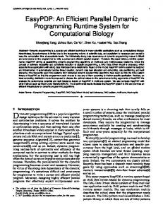
Figure 1. A simplified diagram of DCS block and WGD.

conserved over different organisms [16, 17, 18]. A typical example for this phenomenon can be seen between two yeast-species Kluyveromyces waltii and Saccharomyces cerevisiae [17]. By detecting the doubly conserved synteny (DCS) blocks of the two species, where each region of K. waltii corresponds to one region out of two yeasts in S. cerevisiae, Kellis et al. [17] obtain the support for the whole-genome duplication (WGD) or two rounds of gene duplication (2R) hypothesis [19, 20]. Figure 1 shows a simplified diagram of DCS block and WGD, which is an important application of the merged LCS problem. Another application of the merged LCS problem is the signal comparison. For example, the merged LCS enables one to identify the similarity between a complete voice (one series of signals without noise), and two incomplete voices (two series of signals sampled with different noise). Therefore, detecting the interleaving relationship between sequences is very realistic, for both fixed alphabets (genes) and large alphabets (signals with various values). Note that the alphabet is sortable for most cases. Therefore, for the merged LCS problem, without or with block constraint, it is still worth considering how to improve the existing results [15] by a sparse dynamic programming. However, no existing algorithms can be applied to achieve this goal directly. Though it is also interesting to solve these problems by machine learning [21] or iterative optimization [22, 23], these approaches may not obtain the optimal solution. To ensure that the optimal solution is always obtained, we focus on theoretical improvements of existing results [15]. In this paper, we propose the first known algorithm that solves the merged LCS problem with sparse dynamic programming. The proposed algorithm can be easily extended to solve the block-merged LCS problem. These new algorithms improve Huang’s results [15], especially for sequences over large alphabets. The rest of this paper is organized as follows. Section 2 provides explanations and annotations for the merged LCS problem and the block-merged LCS problem. Section 3 describes a simple linear time strategy for finding two-dimensional minima of nonnegative integer points. In Section 4, we use the result of Section 3 to solve the merged

SPARSE DYNAMIC PROGRAMMING FOR THE MERGED LCS

1937

LCS problem. In Section 5, we extend the algorithms in Section 4 to solve the blockmerged LCS problem. The analysis for large alphabets can be found in the ending part of Section 5. Section 6 concludes and discusses future work.

2. The LCS with Merging Sequences. 2.1. The Merged LCS Problem. Given a target sequence T and two merging sequences A and B, the merged LCS problem, denoted as M LCS(T, A, B), is to determine the LCS of T and A ⊕ B, where ’⊕’ denotes the merging operation which merges A and B into an interleaving sequence. Note that the result of A ⊕ B may not be unique, which means the problem is not trivial. For example, suppose we have A = a1 a2 a3 a4 = actt and B = b1 b2 b3 = ctg, then three of the possible merging sequences are M1 = a1 a2 b1 b2 a3 a4 b3 = acctttg, M2 = a1 a2 a3 a4 b1 b2 b3 = acttctg, and M3 = b1 a1 b2 a2 b3 a3 a4 = catcgtt. Further, suppose that the target sequence is T = tcatcga. Then, by examining all merging sequences, it can be seen that one of the optimal solutions of M LCS(T, A, B) is LCS(T, M3 ) = catcg, whose length is 5. This example illustrates that the MLCS approach is useful for measuring the interleaving relationship between sequences. Based on dynamic programming, Huang et al. give an on-line O(nmr)-time algorithm [15] for determining M LCS(T, A, B), whose off-line implementation requires O(mr) space, where n, m and r denote the length of T , the longer and shorter lengths of A and B, respectively. In Section 4, we propose an improved O(Lnr)-time on-line algorithm for solving M LCS(T, A, B), whose off-line implementation requires O(m + Lr) space, where L = |M LCS(T, A, B)| denotes the length of the optimal solution for the merged LCS problem. For any alphabet whose size is asymptotically linear to m, our improvement is √ significant because O(L) is expected as O( m) [24]. Also, our O(Lnr)-time algorithm achieves the best known result when L is relatively small. 2.2. The Block-merged LCS Problem. For genomic or signal comparison that is restricted with block constraints [17], Huang et al. further propose the block-merged LCS model. Different from the merged LCS problem, the block-merged LCS problem asks for the LCS of T and A ⊗ B, defined as M LCS # (T, A, B), where ’⊗’ denotes the merging operation with blocks. To give an example, let A= actt, as in the previous example. Now we divide A = actt into two blocks X1 = ac# and X2 = tt#, represented as A = X1 X2 = ac#tt#, where ′ #′ denotes the dividing symbol that ends a block. Suppose B = ctg is also divided into two blocks B = Y1 Y2 = ct#g#. In this case, three of the possible merging sequences with blocks are M1# = X1 Y1 X2 Y2 = acctttg, M2# = X1 X2 Y1 Y2 = acttctg, and M3# = Y1 X1 Y2 X2 = ctacgtt. Similarly, by checking all merging sequences of A ⊗ B, one can see that both LCS(T, M2# ) = atcg and LCS(T, M3# ) = ctcg are optimal solutions of M LCS # (T, A, B). Note that for this case, the merging sequence M3 = b1 a1 b2 a2 b3 a3 a4 in our previous example cannot be obtained from A ⊗ B, because M3 breaks the blocks. By considering the ends of blocks, Huang et al. derive an O(nm(|A# | + |B # |))-time on-line algorithm [15] for solving the block-merged LCS problem, where |A# | and |B # | denote the number of blocks in A and B, respectively. In addition, by using the technique of S-table [25, 26], they further propose an off-line algorithm that requires only O(nm + n|A# ||B # |) time and space. Let L′ = |M LCS # (T, A, B)| be the length of the optimal solution for the block-merged LCS problem. In Section 5, we will explain how to determine M LCS # (T, A, B) with O(min{L′ n(|A# | + |B # |), n(|A# |r + |B # |m)}) time and O(m + L′ (|A# | + |B # |)) space.

1938

Y.-H. PENG, C.-B. YANG, K.-S. HUANG, C.-T. TSENG AND C.-Y. HOR

3. The Two-dimensional Minima of Non-negative Integer Points. In this section, we show that the two-dimensional minima of non-negative integer points can be determined efficiently. This property will be used for our algorithm in the next section. The definition of a minimum in a set of two-dimensional points is given as follows. Definition 3.1. Given a set Q of two-dimensional points, a two-dimensional minimum of Q is a point (x, y) ∈ Q such that x′ > x or y ′ > y, for any point (x′ , y ′ ) ∈ Q − {(x, y)}. When the points in Q are integer points with boundaries, the set of two-dimensional minima in Q, defined as M IN (Q), can be determined with bucket sort. Let each point in Q be bounded by non-negative integers Zx and Zy , which means that 0 ≤ x ≤ Zx and 0 ≤ y ≤ Zy , for any (x, y) ∈ Q. In this case, we have the following result.

Lemma 3.1. For any set Q of two-dimensional integer points bounded by non-negative integers Zx and Zy , the determination of M IN (Q) can be achieved in O(|Q|+min(Zx , Zy )) time.

Proof: Without loss of generality, suppose Zx ≤ Zy . Applying the bucket sort with respect to x-axis, it takes O(|Q| + Zx ) time to divide Q into (Zx + 1) sets Q0 , Q1 , · · · , QZx . Since it takes O(|Qi |) time to determine the unique two-dimensional minimum M IN (Qi ) = (i, yi ), for 0 ≤ i ≤ Zx , the overall time for determining all such (i, yi ) would be O(|Q|+Zx ). If Qi is an empty set, then (i, yi ) = (∞, ∞). Now, it is clear that M IN (Q) can be obtained with an O(Zx )-time linear scan on M IN (Q0 ), M IN (Q1 ), · · · , M IN (QZx ). Therefore, the lemma holds. For the case of real points, known sorting algorithms allow M IN (Q) to be determined in O(|Q| log |Q|) time. Here we omit the algorithm for real points, because Lemma 3.1 is sufficient to support our algorithms in Section 4. 4. Algorithms for the Merged LCS Problem. In this section, we solve the merged LCS problem in O(Lnr) time. Briefly, our algorithm solves the problem by locating proper indices (candidates) with two-dimensional minima. To improve the efficiency of our algorithm, we also show how to reduce the space complexity to O(min{Lnr, Lmr}) for on-line applications, and O(m + Lr) for off-line applications. 4.1. Locating Candidates. For a sequence S, let S[i] denote the ith character in S. Also, let S[i, j] denote the substring in S that ranges from S[i] to S[j], for any 1 ≤ i ≤ j ≤ |S|. Further, define S[0] as an empty character and S[i, j] as an empty string for any i > j. Also, let S1 + S2 denote the concatenated sequence for two sequences S1 and S2 . In addition, we define the relationship between a pair of distinct 2-tuple numbers as follows. Definition 4.1. Given a pair of 2-tuple numbers (i, j) and (i′ , j ′ ), we say that (i′ , j ′ ) < (i, j) if i′ ≤ i and j ′ ≤ j for (i, j) 6= (i′ , j ′ ).

In the following, we explain the idea of identifying candidates. Suppose we have the target sequence T = t1 t2 · · · tn , two merging sequences A = a1 a2 · · · am and B = b1 b2 · · · br with m ≥ r. An (l, k)-candidate is defined as follows.

Definition 4.2. For 0 ≤ i ≤ m, 0 ≤ j ≤ r and 0 ≤ l ≤ k ≤ n, a pair of integers (i, j) is an (l, k)-candidate if the following conditions hold. (1)|M LCS(T [1, k], A[1, i], B[1, j])| = l (2)For any integer (i′ , j ′ ) < (i, j), |M LCS(T [1, k], A[1, i′ ], B[1, j ′ ])| < l. Such an (l, k)candidate is also called a dominating candidate. According to Definition 4.2, there exist some (L, k)-candidates (i, j) such that L = |M LCS(T [1, k], A[1, i], B[1, j])| = |M LCS(T, A, B)|, for 0 ≤ k ≤ n, 0 ≤ i ≤ m and 0 ≤ j ≤ r. Based on this idea, a lemma follows.


1939

Lemma 4.1. There exists an increasing sequence of dominating candidates C = (i0 , j0 ) < (i1 , j1 ) < · · · < (iL , jL ) and indices K = k0 , k1 , · · · , kL , where i0 = j0 = k0 = 0, such that (ip , jp ) is a (p, kp )-candidate, 0 ≤ p ≤ L, and T [k1 ], T [k2 ], · · · , T [kL ] is the LCS of T and A ⊕ B. Proof: The correctness of this lemma can be verified with recursion. In the following, we explain how to construct these dominating candidates and indices efficiently, so as to determine the LCS of T and A ⊕ B. 4.2. The On-line Algorithm for Merged LCS. We first introduce some notations. For any symbol σ, let nextA (σ, i) = i′ denote the minimum index i′ > i in sequence A such that A[i′ ] = σ. If there is no such index, set i′ = ∞. Also, let nextB (σ, j) serve the same purpose for sequence B. Suppose the alphabet is of fixed size. Thus, with an O(m + r)time preprocessing that constructs a mapping table on A and B, both nextA (σ, i) and nextB (σ, j) can be determined in constant time, for any 0 ≤ i ≤ m, 0 ≤ j ≤ r. Let ′ Hl,k denote the set of (l, k)-candidates. Also, let Hl,k be a set constructed by substituting each (i, j) ∈ Hl,k with two integer points (nextA (T [k + 1], i), j) and (i, nextB (T [k + 1], j)). ′ ′ Any point (x, y) ∈ Hl,k is excluded from Hl,k if x = ∞ or y = ∞. Hence, we have ′ ′ |Hl,k | ≤ 2|Hl,k |. Note that each (x, y) in Hl,k is now bounded by Zx = |A| = m and Zy = |B| = r. Besides, Hl,k can also be deemed as a set of integer points bounded by Zx = m and Zy = r. Algorithm 1 Finding the merged LCS in O(Lnr) time Set len ← 1 and H0,k ← {(0, 0)}, for 0 ≤ k ≤ n. for k = 1 to k = n do for l = 1 to l = len do ′ Construct Hl−1,k−1 from Hl−1,k−1 with next ′ Hl,k ← M IN (Hl−1,k−1 ∪ Hl,k−1 ) end for if |Hlen,k | > 0 then len ← len + 1 end if end for L ← len − 1 Retrieve the LCS by tracking from HL,n to H0,0 . Algorithm 1 provides an online method for solving the merged LCS problem in O(Lnr) time. To prove the correctness of Algorithm 1, in the following we derive some useful properties of dominating candidates. Lemma 4.2. For any dominating candidate (i, j) ∈ Hl,k with l ≥ 1 and k ≥ 1, one of the following conditions holds. (1)There exists (¯i, ¯j) ∈ Hl−1,k−1 such that i = nextA (T [k], ¯i) and j = ¯j. (2)There exists (¯i, ¯j) ∈ Hl−1,k−1 such that i = ¯i and j = nextB (T [k], ¯j). (3)There exists (¯i, ¯j) ∈ Hl,k−1 such that i = ¯i and j = ¯j. Proof: The proof of this lemma can be done by discussing whether T [k] is picked as the lth common character, for each candidate (i, j) ∈ Hl,k . If T [k] is picked as the lth common character, then T [k] must be picked with either A[i] or B[j]. Otherwise, there will be some integers i′ ≤ i − 1, j ′ ≤ j − 1 such that |M LCS(T [1, k], A[1, i′ ], B[1, j ′ ])| = l, which is contradictory to that (i, j) is an (l, k)-candidate. Clearly, picking T [k] with A[i]

1940


or B[j] leads to condition (1) or (2), respectively. Also, one can see that condition (3) holds if T [k] is not picked as the lth common character. ′ Combining Definitions 3.1, 4.2 and Lemma 4.2, we have Hl,k = M IN (Hl−1,k−1 ∪Hl,k−1 ), ′ which is the set of minima in Hl−1,k−1 ∪ Hl,k−1 . In the following, we shall show that each Hl,k can be obtained in O(r) time. Lemma 4.3. For 1 ≤ l ≤ L and 1 ≤ k ≤ n, Hl,k can be obtained in O(r) time when Hl−1,k−1 and Hl,k−1 are given. Proof: With the pigeonhole principle, one can see that both Hl−1,k−1 and Hl,k−1 contain ′ ′ no more than r +1 candidates. Because |Hl−1,k−1 | ≤ 2|Hl−1,k−1 |, it is clear that |Hl−1,k−1 ∪ ′ Hl,k−1 | ≤ 3(r + 1). With Lemma 3.1, Hl,k can be obtained in O(|Hl−1,k−1 ∪ Hl,k−1 | + min(m, r)) = O(r) time. By Lemmas 4.2 and 4.3, one can see that Algorithm 1 determines HL,n in O(Lnr) time. Based on Lemma 4.1, it is easy to design an O(L + n)-time backtracking algorithm for Algorithm 1. With additional analysis for the required space, our first result is given in Theorem 4.1. Theorem 4.1. M LCS(T, A, B) can be determined on-line respect to T with O(Lnr) time and O(min{Lnr, Lmr}) space. Proof for the space complexity: Given (i, j) ∈ Hl,k , let Backl,k (i, j) denote the query function for tracking the previous dominating candidate which generates (i, j). That is, we have Backl,k (i, j) = (i′ , j ′ ) if (i, j) is generated by (i′ , j ′ ) ∈ Hl−1,k−1 , satisfying either (nextA (T [k], i′ ), j ′ ) = (i, j) or (i′ , nextB (T [k], j ′ )) = (i, j). Otherwise, we have Backl,k (i, j) = (i, j) because (i, j) ∈ Hl,k is generated by (i, j) ∈ Hl,k−1 . A straightforward implementation would fully update the tracking function O(Lnr) times, which requires O(Lnr) space to retrieve the LCS. However, the tracking function need not be updated with Backl,k (i, j) = (i′ , j ′ ) if for any k ′ < k there already exists (i, j) ∈ Hl,k′ . That is, the query Backl,k (i, j) can be replaced with Backl,k′ (i, j), if a common subsequence of length l can be obtained from T [1, k ′ ] and A[1, i] ⊕ B[1, j], for any k ′ < k. One can see that with Backl,k′ (i, j), the retrieved LCS is still of length l. Therefore, for any triplet (i, j, l), we need to update the tracking function only one time for the minimum k that (i, j) ∈ Hl,k , denoted as M K(i, j, l). Since the number of (i, j, l)triplets is bounded by O(Lmr), the required space for storing the tracking function is also bounded by O(Lmr). Note that all Backl,k and M K can be implemented with a table of (m + 1) × (r + 1) grids, where each grid Gi,j contains a linked list which stores each M K(i, j, l) with increasing l. That is, the lth element in Gi,j stores the minimum k such that (i, j) ∈ Hl,k . Therefore, to update Backl,k (i, j) = (i′ , j ′ ), one can first append to Gi,j a new element which stores k, then add a link from the last (lth) element in Gi,j to the last ((l − 1)th) element in Gi′ ,j ′ , which takes constant time. The correctness of this implementation can be verified with the observation that for any (i, j) ∈ H¯l,k¯ and (i, j) ∈ Hl,k which result in two different updates, we have ¯l < l if and only if k¯ < k. Therefore, the upper bound of the required space is linear to the total number of generated pairs, which is known to be O(Lnr). Note that building the table of (m + 1) × (r + 1) grids takes Ω(mr) time and space. Therefore, the required time and space are O(Lnr + mr) and O(min{Lnr + mr, Lmr}), respectively. However, for on-line applications it is suitable to assume Ln > m, since n still grows whereas m is given. Therefore, by omitting the additional O(mr) complexity, one can see that the theorem holds. Our backtracking algorithm is summarized as Algorithm 2, which serves as the supplement to Algorithm 1. One can see that Algorithm 2 retrieves the LCS in O(L) time,


1941

which is also an improvement to the O(n + L)-time straightforward implementation. The space efficiency of Theorem 4.1 would also be substantial for on-line applications when n is much greater than m. Algorithm 2 Retrieving the LCS in O(L) time Set l ← L and k ← n. Pick an arbitrary candidate (i, j) ∈ HL,n . while l 6= 0 do k ← M K(i, j, l) (i′ , j ′ ) ← Backl,k (i, j) if i′ < i then Report A[i] and T [k] as the lth common character. else Report B[j] and T [k] as the lth common character. end if (i, j) ← (i′ , j ′ ) l ←l−1 end while 4.3. The Off-line Implementation. If the on-line process on T is not required, we can give a more space-efficient implementation with O(m+Lr) space, provided that the length of T is given beforehand. Though, under this assumption, the proposed algorithm becomes off-line to T , an O(m + Lr)-space implementation is necessary in some circumstances. Briefly, our off-line algorithm is an extension to Hirschberg’s divide-and-conquer algorithm [1]. However, we avoid the reverse computation. This makes our algorithm easy to implement. Theorem 4.2. M LCS(T, A, B) can be determined with O(Lnr) time and O(m + Lr) space. P Proof: Note that for any specific k, we have Ll=1 |Hl,k | ≤ L(r + 1). That is, it takes O(Lr) space to store all Hl,⌊ n2 ⌋ , for 1 ≤ l ≤ L. Here we treat the case L = 0 as the ′ boundary condition that needs no further tracking. Since Hl,k = M IN (Hl−1,k−1 ∪ Hl,k−1 ), any tracking path from H1≤l≤L,⌊ n2 ⌋≤k≤n to H0,0 must pass through a unique dominating candidate (ib , jb ) ∈ Hlb ,⌊ n2 ⌋ with a unique length lb , 0 ≤ lb ≤ L. In other words, this unique (ib , jb ) can be used as the breaking point in Hirschberg’s divide-and-conquer strategy. Let M idl,k (i, j) denote such a unique dominating candidate obtained by tracking from (i, j) ∈ Hl,k≥⌊ n2 ⌋ to H0,0 . Next, with the following formulas, we show how to obtain M idl,k (i, j) without reverse computation. (1)M idl,⌊ n2 ⌋ (i, j) = (i, j). (2)For ⌊ n2 ⌋ < k ≤ n, M idl,k (i, j) = M idl,k−1 (i, j) if (i, j) ∈ Hl,k and (i, j) ∈ Hl,k−1 . (3)Otherwise, let (i′ , j ′ ) = Backl,k (i, j), we have M idl,k (i, j) = M idl−1,k−1 (i′ , j ′ ). The correctness of the above formula can be easily seen, since it is a simple strategy which passes down the information of the demanded candidates. For all candidates (î, ˆj) ∈ HL,n , M idL,n (î, ˆj) can be obtained with O(Lnr) time and O(Lr)-space. Suppose (ib , jb ) ∈ Hlb ,⌊ n2 ⌋ = M idL,n (î, ˆj) is the demanded candidate for some (î, ˆj) ∈ HL,n . Let Tα = T [1, ⌊ n2 ⌋ − 1], Tβ = T [⌊ n2 ⌋ + 1, n], Aα = A[1, ib ], Aβ = A[ib + 1, m], Bα = B[1, jb ], Bβ = B[jb + 1, r] be six divided sequences, the problem can now be split according to different conditions.

1942


(1)If (ib, jb) ∈ Hlb ,⌊ n2 ⌋−1, then we have |M LCS(T [1, ⌊ n2 ⌋ − 1], A[1, ib ], B[1, jb ])| = lb and |M LCS(T [⌊ n2 ⌋ + 1, n], A[ib + 1, m], B[jb + 1, r])| = L − lb . That is, M LCS(T, A, B) can be solved by computing M LCS(Tα , Aα , Bα )+M LCS(Tβ , Aβ , Bβ ). Note that it takes only constant time to determine whether (ib , jb ) is in Hlb ,⌊ n2 ⌋−1 , since one can pass down the answer along with the M id function. (2)If (ib, jb) ∈ / Hlb ,⌊ n2 ⌋−1, then based on the proof of Lemma 4.1, either A[ib ] or B[jb ] must be picked with T [⌊ n2 ⌋] to form the lb th common character. Suppose A[ib ] is picked, then the whole longest common subsequence M LCS(T, A, B) must be of the form M LCS(Tα , Aα [1, ib − 1], Bα ) + T [⌊ n2 ⌋] + M LCS(Tβ , Aβ , Bβ ). Similarly, one can see that M LCS(T, A, B) = M LCS(Tα , Aα , Bα [1, jb − 1]) + T [⌊ n2 ⌋] + M LCS(Tβ , Aβ , Bβ ) if B[jb ] is picked. With properties |Tα | ≤ ⌊ n2 ⌋, |Tβ | ≤ ⌊ n2 ⌋, |Aα | + |Aβ | = m, |Bα | + |Bβ | = r and lb + (L − lb ) = L, we get that rlb |Tα | + r(L − lb )|Tβ | ≤ Lnr . 2 The above discussion indicates that the overall time for solving the subproblems is always bounded by half of that needed to solve M LCS(T, A, B). Therefore, this implementation takes O(Lnr) time but O(Lr) space. Note that it still takes O(m + r) space to construct the functions nextA and nextB . Therefore, the overall space complexity is O(m + r + Lr) = O(m + Lr). In the worst case, this off-line implementation takes no more than O(mr) space, because L ≤√2m. In some cases, however, the required space is much less. If, for example, L = r = m, then our implementation takes only O(m) space, rather than O(mr) = O(m1.5 ) space. In addition, for the case that L is relatively small, the required space reduces to near O(m + r). 5. Extending the Algorithm with Block Constraints. In this section, we show how to extend the algorithms proposed in the previous section to solve the problem with block constraints. Our extension is done by first relating M LCS # (T, A, B) to dominating candidates, and then showing that these new dominating candidates can still be obtained with a similar sparse dynamic programming. 5.1. Candidates with Block Constraints. Recall that the symbol ′ #′ means the end of a block. To fit the problem, we assume that ’#’ does not appear in T , and that each block ends with a dividing symbol. That is, we have A[m]=’#’ and B[r]=’#’ if both A and B contain at least one block. For the case of an empty block, we assume it ends # with an empty character. For any A[i] 6=’#’ and B[j] 6=’#’, let num# A (i) and numB (j) denote the number of ’#’s in A[1, i] and B[1, j], respectively. That is, for any 1 ≤ i ≤ m, num# A (i) means the block index in A where A[i] can be located. Therefore, A[i1 ] and A[i2 ] # are in the same block if and only if num# A (i1 ) = numA (i2 ), for 1 ≤ i1 , i2 ≤ m. In T , let k1 ≤ k ′ ≤ k2 be three arbitrary indices of the LCS obtained from T and A ⊗ B. Clearly, any LCS obtained from T and A ⊗ B must satisfy the following two conditions: (1)For any A[i1 ] and A[i2 ] picked with T [k1 ] and T [k2 ], respectively, T [k ′ ] cannot be picked # with any B[j], for 1 ≤ j ≤ r, if num# A (i1 ) = numA (i2 ). (2)For any B[j1 ] and B[j2 ] picked with T [k1 ] and T [k2 ], respectively, T [k ′ ] cannot be # picked with any A[i], for 1 ≤ i ≤ m, if num# B (j1 ) = numB (j2 ). Let K ′ = k0′ , k1′ , k2′ , · · · kL′ ′ be some indices of T such that T [k1′ ], T [k2′ ], · · · , T [kL′ ′ ] is an LCS obtained from M LCS # (T, A, B). For L′ = 0, let k0′ = 0 represent the empty index which means no common subsequence can be found between T and A ⊗ B. The following lemma describes the relationship between M LCS # (T, A, B) and dominating candidates. Lemma 5.1. For any sequence of indices K ′ = k0′ , k1′ , k2′ , · · · kL′ ′ where T [k1′ ], T [k2′ ], · · · , T [kL′ ′ ] is an LCS obtained from M LCS # (T, A, B), there exists a sequence of pairs C # =


1943

′ (i′0 , j0′ ), (i′1 , j1′ ), (i′2 , j2′ ), · · · , (i′L′ , jL′ ′ ) such that for 1 ≤ p ≤ L′ , (1)(i′p−1 , jp−1 ) < (i′p , jp′ ) and (2)for each (i′p , jp′ ) ∈ C # , one of A[i′p ] and B[jp′ ] serves as the pth common character with T [kp′ ] while the other must be a dividing symbol ’#’ or an empty character.

Proof: This lemma can be verified by a recursion considering block constraints. To support the algorithm we are to describe, we give a conditional definition of X ⊗ Y for two given sequences X and Y , which does not alter Huang’s derivation but will simplify our further presentation. Let X ′ and Y ′ denote the longest prefixes of X and Y that end with ’#’, respectively. Definition 5.1. (1)If |X| = 0 or |Y | = 0, let X ⊗ Y = X + Y . (2)For X[|X|]=’#’ and Y [|Y |]=’#’, let X ⊗ Y denote a merged sequence of X and Y with block constraints. (3)For X[|X|] 6=’#’ and Y [|Y |] =’#’, let X ⊗ Y = (X ′ ⊗ Y ) + X[|X ′ | + 1, |X|]. (4)For X[|X|] =’#’ and Y [|Y |] 6=’#’, let X ⊗ Y = (X ⊗ Y ′ ) + Y [|Y ′ | + 1, |Y |].

The first two conditions in Definition 5.1 describe Huang’s derivation of block constraints [15], while the third and the fourth conditions are mainly used for supporting our algorithm. Definition 5.1 does not consider the case where both X[|X|] ∈ / {’#’, φ} and Y [|Y |] ∈ / {’#’, φ}, because it will be excluded by the following definition of an (l, k)# candidate. Definition 5.2. For 0 ≤ i ≤ m, 0 ≤ j ≤ r and 0 ≤ l ≤ k ≤ n, a pair of integers (i, j) is called an (l, k)# -candidate if the following three conditions hold. (1)A[i] ∈ {’#’, φ} or B[j] ∈ {’#’, φ}. (2)|M LCS # (T [1, k], A[1, i], B[1, j])| = l (3)For any pair of integers (i′ , j ′ ) where A[i′ ] ∈ {’#’, φ} or B[j ′ ] ∈ {’#’, φ}, |M LCS # (T [1, k], A[1, i′ ], B[1, j ′ ])| < l if (i′ , j ′ ) < (i, j). In fact, Definition 5.2 is an extension of Definition 4.2 to include block constraints. 5.2. Extended On-line and Off-line Algorithms. Now we explain how to determine M LCS # (T, A, B) by a sparse dynamic programming that locates candidates. The new sparse dynamic programming is obtained with a slight modification to the result of Section # ′# 4. Let Hl,k denote the set of (l, k)# -candidates. Also, let Hl,k be the set obtained by # replacing each candidate (i, j) ∈ Hl,k with two pairs of integers according to the following rules. (1)For (i, j) = (0, 0): Replace (i, j) by (0, nextB (T [k + 1], 0)) and (nextA (T [k + 1], 0), 0). (2)For A[i] ∈ / {’#’, φ}: Replace (i, j) by (nextA (T [k + 1], i), j) and (nextA (’#’, i), nextB (T [k + 1], j)). (3)For B[j] ∈ / {’#’, φ}: Replace (i, j) by (i, nextB (T [k + 1], j)) and (nextA (T [k + 1], i), nextB (’#’, j)). ′# # Any (x, y) ∈ Hl,k is excluded if x = ∞ or y = ∞. Here we have |Hl,k | ≤ (|A# |+|B # |+2), # ′# # because for each (i, j) ∈ Hl,k , either A[i] or B[j] is an end of block. Since |Hl,k | ≤ 2|Hl,k |, # ′# # # both |Hl,k | and |Hl,k | are bounded by O(|A | + |B |). Based on the idea in Section 4, # can be constructed recursively. each Hl,k # ′# # Lemma 5.2. Hl,k = M IN (Hl−1,k−1 ∪ Hl,k−1 ), for 1 ≤ l ≤ k ≤ n.

Proof: This lemma is correct based on the result of Section 4. # Nonetheless, note that Lemma 3.1 cannot be directly applied to obtain Hl,k , since it ′# # # # # still takes O(|A |+|B |+r) time even if |Hl−1,k−1 ∪Hl,k−1 | is bounded by O(|A |+|B # |). # In the following, we propose the last trick, which guarantees that Hl,k can be obtained in # # O(|A | + |B |) time.

1944


# Lemma 5.3. For 1 ≤ l ≤ k ≤ n, each Hl,k can be determined with O(|A# | + |B # |) time # # if both Hl−1,k−1 and Hl,k−1 are given.

Proof: Let QA0 , QA1 , QA2 , · · · , QA|A# | and QB0 , QB1 , QB2 , · · · , QB|B# | denote distinct sets

′# # of integer pairs which are constructed from Hl−1,k−1 ∪ Hl,k−1 with the following two rules. ′# # (1)For any (i, j) ∈ Hl−1,k−1 ∪ Hl,k−1 , if A[i] ∈ {’#’φ}, then (i, j) ∈ QAI , where I = num# A (i). (2)Otherwise, we have B[j] ∈ {’#’φ} and (i, j) ∈ QBJ , where J = num# B (j). ′# # # Based on these rules, one can partition Hl−1,k−1 ∪ Hl,k−1 into (|A | + |B # | + 2) sets in O(|A# | + |B # |) time. Keeping the minimum pair in each QAI and QBJ , one can then perform an O(|A# | + |B # |)-time linear scan to obtain two sets of 2D minima QA = M IN (QA0 ∪ QA1 ∪ · · · ∪ QA|A# | ) and QB = M IN (QB0 ∪ QB1 ∪ · · · ∪ QB|B# | ). Since both QA and QB are 2D minima, they are two sorted sets of points with respect to the x-coordinate. That is, it takes O(|QA | + |QB |) time to merge QA and QB into a set QM so that QM is also sorted with respect to the x-coordinate. Therefore, M IN (QM ) can be obtained by an O(|QM |)-time linear scan on QM . This means M IN (QM ) can be determined in ′# # # O(|A# | + |B # |) time. Since we have M IN (QM ) = M IN (Hl−1,k−1 ∪ Hl,k−1 ) = Hl,k , we conclude that the lemma holds. Definition 5.2 reveals that for any specific k and l1 6= l2 , Hl#1 ,k ∩ Hl#2 ,k = {φ}. Therefore, PL′ # ′ # # # # l=0 |Hl,k | is bounded by both O(L (|A | + |B |)) and O(|A |r + |B |m). According to Lemma 5.3, it is not difficult to design an O(min{L′ n(|A# | + |B # |), n(|A# |r + |B # |m)})time algorithm for determining HL#′ ,n (see Algorithm 1). With the concept of Theorem 4.1, one can easily verify the correctness of the following theorem, thus its proof is omitted.

Theorem 5.1. M LCS # (T, A, B) can be determined on-line respect to T with O(min{L′ n(|A# |+|B # |), n(|A# |r+|B # |m)}) time and O(min{L′ n(|A# |+|B # |), L′ (|A# |r +|B # |m)}) space. Note that both O(L′ n(|A# | + |B # |)) and O(n(|A# |r + |B # |m)) are necessary for measuring the time complexity. Taking r = log n, |A# | = m and |B # | = 1 for example, we have O(L′ n(|A# | + |B # |)) = O(L′ nm) but O(n(|A# |r + |B # |m)) = O(nm log n). The required space of this example is only O(L′ m log n), which is a substantial improvement for the case where n > m. For off-line applications, Hirschberg’s idea [1] can still be applied to reduce the space complexity. Based on the proof of Theorem 4.2, the following result can be easily obtained. Theorem 5.2. M LCS # (T, A, B) can be determined with O(min{L′ n(|A# | + |B # |), n(|A# |r + |B # |m)}) time and O(m + L′ (|A# | + |B # |)) space. For applications that both |A# | and |B # | are relatively small, our algorithm takes only O(L′ n) time. In contrast, previous algorithm with S-table [15] does not meet this bound. Consider two sequences A = X1 , X2 , · · · , X|A# | and B = Y1 , Y2 , · · · , Y|B # | , where each Xi ∈ A denotes a single block and each Yj ∈ B does, too. The construction of S-tables P # | A P|B # | B A B takes Ω( |A i=1 nLi + j=1 nLj ) time and space, where Li and Lj denote |LCS(T, Xi )| P|A# | A P|B # | B and |LCS(T, Yj )|, respectively. Obviously, we have ( i=1 Li + j=1 Lj ) ≥ L′ . Therefore, the needed time for computing S-tables cannot be kept in O(L′ n). Theorem 5.2 also indicates that our algorithm is more space-efficient than S-tables, since we have (|A# | + |B # |) < n in general. When the number of blocks is limited, our off-line algorithm takes only O(m) space.


1945

Table 1. Algorithms for the merged LCS and the block-merged LCS problem. Here, n, m and r denote the length of T , the longer and shorter lengths of A and B, respectively, L or L′ denotes the length of the answer, and δ denotes the number of blocks in A and B. Algorithm Huang’s on-line [15] Our on-line Huang’s off-line [15] Our off-line Algorithm Huang’s on-line [15] Our on-line Huang’s off-line [15] Our off-line

Merged LCS Complexity Fixed Alphabets Time O(nmr) Space O(nmr) Time O(Lnr) Space O(Lmr) Time O(nmr) Space O(mr) Time O(Lnr) Space O(m + Lr) Block-merged LCS Complexity Fixed Alphabets Time O(nmδ) Space O(nmδ) Time O(L′ nδ) Space O(L′ mδ) Time O(nm + nδ 2 ) Space O(nm + nδ 2 ) Time O(L′ nδ) Space O(m + L′ δ)

Large Alphabets O(nmr) O(nmr) √ O(n mr) O(m1.5 r) O(nmr) O(mr) √ O(n mr) √ O(m + mr) Large Alphabets O(nmδ) O(nmδ) √ O(n mδ) O(m1.5 δ) O(nm + nδ 2 ) O(nm + nδ 2 ) √ O(n mδ) √ O(m + mδ)

5.3. Analysis for Large Alphabets. In this subsection, we give a brief analysis for the case of large alphabets. Let |ΣA | ≤ m and |ΣB | ≤ r denote the number of distinct symbols in A and B, respectively. Thus, |Σ| = |ΣA ∪ ΣB | ≤ m + r, where Σ denotes the overall alphabet. In this case, it takes O(|Σ| log |Σ| + |ΣA |m + |ΣB |r) time and O(|ΣA |m + |ΣB |r) space to construct the lexical-ordered tables for storing nextA and nextB . However, note that the constructing time and space can be reduced to O(m log m) and O(m), respectively, by using (|ΣA | + |ΣB |) arrays that separately store the indices of each symbol in A and B. Therefore, for each T [k], it takes O(log m) time to locate the array of T [k]. Then, each query for nextA (T [k], i) and nextB (T [k], j) can be answered in O(log |T [k]|) time, where |T [k]| denotes number of indices i′ that A[i′ ] = T [k] or B[i′ ] = T [k]. Note m ), which is almost a constant for large alphabets. In that |T [k]| is expected as O( |Σ| √ addition, recall that for large alphabets, O(L) is expected to be O( m) [24]. Therefore, our algorithms achieve significant improvements for large alphabets. 6. Conclusions. Table 1 summarizes related results for the merged LCS problem and the block-merged LCS problem. In Table 1, we adopt the general case that O(n) = O(m). However, we do not replace each m with n, because they have different meaning in the problem. In addition, for simplicity, we assume O(|A# |) = O(|B # |) = O(δ) ≤ O(m). For large alphabets, we assume m = c|Σ|, √ for somemconstant c, by which we apply the ) = O(1) [24]. expected case that O(L′ ) ≤ O(L) = O( m) and O( |Σ| In Table 1, most of our algorithms are more efficient than previous results. Here we briefly discuss the only exception: our off-line algorithm for the block-merged LCS problem with fixed alphabets. In this case, for O(L′ δ) ≥ O(m + δ 2 ), our algorithm would be less efficient in time. However, one should note that our off-line algorithm is always more efficient in space. Therefore, it is suitable for one to design a hybrid algorithm that combines our results with Huang’s. For future study, here is an interesting problem. Recall that our on-line algorithms for solving M LCS(T, A, B) and M LCS # (T, A, B) require O(min{Lnr, Lmr}) space and

1946


O(min{L′ n(|A# |+|B # |), L′ (|A# |r+|B # |m)}) space, respectively. The space complexities for the average case, however, have not yet been analyzed. A few simple tests even suggest that our analysis for the worst cases may not be tight. For example, suppose that T =an , A =an and B =an are three identical sequences of length n, which are formed with a unique symbol ’a’. This is one of the worst cases for traditional on-line sparse dynamic programming to determine LCS(T, A) and LCS(T, B), because the number of matches is maximized. By the implementation of our on-line algorithm with O(min{Lnr, Lmr})space in Section 4, nevertheless, this case requires merely O(n2 ) space, rather than the worst O(n3 ) space. Since the worst case cannot be derived by simply maximizing the number of matches, to propose a tighter space analysis for our on-line algorithms would be an interesting topic in the future. Acknowledgment. This research work was partially supported by the National Science Council of Taiwan under contract NSC-96-2221-E-110-010. The authors gratefully acknowledge the helpful comments and suggestions of Steve Haga and the reviewers, which have improved the presentation. REFERENCES [1] D. S. Hirschberg, “A linear space algorithm for computing maximal common subsequences,” Communications of the ACM, vol. 18, pp. 341–343, 1975. [2] C.-B. Yang and R. C. T. Lee, “Systolic algorithms for the longest common subsequence problem,” Journal of the Chinese Institute of Engineers, vol. 10(6), pp. 691–699, 1987. [3] C. S. Iliopoulos and M. S. Rahman, “New efficient algorithms for the lcs and constrained lcs problems,” Information Processing Letters, vol. 106(1), pp. 13–18, 2008. [4] B. S. Baker and R. Giancarlo, “Sparse dynamic programming for longest common subsequence from fragments,” Journal of Algorithms, vol. 42, no. 2, pp. 231–254, 2002. [5] D. S. Hirschberg, “Algorithms for the longest common subsequence problem,” Journal of the ACM, vol. 24(4), pp. 664–675, 1977. [6] J. W. Hunt and T. G. Szymanski, “A fast algorithm for computing longest common subsequences,” Communications of the ACM, vol. 20(5), pp. 350–353, 1977. [7] J. D. Ullman, A. V. Aho, and D. S. Hirschberg, “Bounds on the complexity of the longest common subsequence problem,” Journal of the ACM, vol. 23(1), pp. 1–12, 1976. ¨ [8] A. N. Arslan and Omer E˘ g ecio˘ g lu, “Algorithms for the constrained longest common subsequence problems,” International Journal of Foundations of Computer Science, vol. 16(6), pp. 1099–1109, 2005. [9] F. Y. L. Chin, A. De Santis, A. L. Ferrara, N. L. Ho, and S. K. Kim, “A simple algorithm for the constrained sequence problems,” Information Processing Letters, vol. 90, pp. 175–179, 2004. [10] C.-L. Lu and Y.-P. Huang, “A memory-efficient algorithm for multiple sequence alignment with constraints,” Bioinformatics, vol. 21(1), pp. 20–30, 2005. [11] Y.-T. Tsai, “The constrained common sequence problem,” Information Processing Letters, vol. 88, pp. 173–176, 2003. [12] Z. Gotthilf, D. Hermelin, and M. Lewenstein, “Constrained LCS: hardness and approximation,” in Combinatorial Pattern Matching, 19th Annual Symposium (CPM2008), (Pisa, Italy), pp. 255–262, 2008. [13] K.-S. Huang, C.-B. Yang, K.-T. Tseng, Y.-H. Peng, and H.-Y. Ann, “Dynamic programming algorithms for the mosaic longest common subsequence problem,” Information Processing Letters, vol. 102, pp. 99–103, 2007. [14] G. A. Komatsoulis and M. S. Waterman, “Chimeric alignment by dynamic programming: algorithm and biological uses,” in RECOMB ’97: Proceedings of the first annual international conference on computational molecular biology, (New York, NY, USA), pp. 174–180, ACM Press, 1997. [15] K.-S. Huang, C.-B. Yang, K.-T. Tseng, H.-Y. Ann, and Y.-H. Peng, “Efficient algorithms for finding interleaving relationship between sequences,” Information Processing Letters, vol. 105(5), pp. 188– 193, 2008. [16] O. Jaillon, J.-M. Aury, F. Brunet, J.-L. Petit, N. Stange-Thomann, E. Mauceli, L. Bouneau, C. Fischer, C. Ozouf-Costaz, A. Bernot, S. Nicaud, D. Jaffe, S. Fisher, G. Lutfalla, C. Dossat, B. Segurens,


[17] [18]

[19] [20] [21]

[22]

[23]

[24] [25] [26]

1947

C. Dasilva, M. Salanoubat, M. Levy, N. Boudet, S. Castellano, V. Anthouard, C. Jubin, V. Castelli, M. Katinka, B. Vacherie, C. Biemont, Z. Skalli, L. Cattolico, J. Poulain, V. de Berardinis, C. Cruaud, S. Duprat, P. Brottier, J.-P. Coutanceau, J. Gouzy, G. Parra, G. Lardier, C. Chapple, K. J. McKernan, P. McEwan, S. Bosak, M. Kellis, J.-N. Volff, R. Guigo, M. C. Zody, J. Mesirov, K. LindbladToh, B. Birren, C. Nusbaum, D. Kahn, M. Robinson-Rechavi, V. Laudet, V. Schachter, F. Quetier, W. Saurin, C. Scarpelli, P. Wincker, E. S. Lander, J. Weissenbach, and H. R. Crollius, “Genome duplication in the teleost fish tetraodon nigroviridis reveals the early vertebrate proto-karyotype,” Nature, vol. 431, no. 7011, pp. 946–957, 2004. M. Kellis, B. W. Birren, and E. S. Lander, “Proof and evolutionary analysis of ancient genome duplication in the yeast saccharomyces cerevisiae,” Nature, vol. 428, no. 6983, pp. 617–624, 2004. D. Vallenet, L. Labarre, Z. Rouy, V. Barbe, S. Bocs, S. Cruveiller, A. Lajus, G. Pascal, C. Scarpelli, and C. Medigue, “MaGe: a microbial genome annotation system supported by synteny results,” Nucleic Acids Research, vol. 34, no. 1, pp. 53–65, 2006. K. Hokamp, A. McLysaght, and K. H. Wolfe, “The 2R hypothesis and the human genome sequence,” Journal of Structural and Functional Genomics, vol. 3, no. 1-4, pp. 95–110, 2003. G. Panopoulou and A. J. Poustka, “Timing and mechanism of ancient vertebrate genome duplications - the adventure of a hypothesis,” TRENDS in Genetics, vol. 21, no. 10, pp. 559–567, 2005. H. Zhu, H. Kai, K. Eguchi, and Z. Guo, “Application of BPNN in classification of time intervals for intelligent intrusion detection decision response system,” International Journal of Innovative Computing Information and Control, vol. 4(10), pp. 2483–2491, 2008. T. Furusho, T. Nishi, and M. Konishi, “Distributed optimization method for simultaneous production scheduling and transportation routing in semiconductor fabrication bays,” International Journal of Innovative Computing Information and Control, vol. 4(3), pp. 559–575, 2008. K. Najim, E. Ikonen, and E. G´ omez-Ramírez, “Trajectory tracking controlbased on a genealogical decision tree controller for robot manipulators,” International Journal of Innovative Computing Information and Control, vol. 4(1), pp. 53–62, 2008. M. Kiwi, M. Loebl, and J. Matou˘ sek, “Expected length of the longest common subsequence for large alphabets,” Advances in Mathematics, vol. 197, pp. 480–498, 2005. G. M. Landau and M. Ziv-Ukelson, “On the common substring alignment problem,” Journal of Algorithms, vol. 41, no. 2, pp. 338–354, 2001. G. M. Landau, B. Schieber, and M. Ziv-Ukelson, “Sparse LCS common substring alignment,” Information Processing Letters, vol. 88, no. 6, pp. 259–270, 2003.