extended in order to (i) cope with partially or fully un- known variable domains; (ii) dynamically acquire do- main values on demand while the constraint propaga-.
Constraint Propagation and Value Acquisition: why we should do it Interactively E.Lamma, P.Mello, M.Milano DEIS University of Bologna V.le Risorgimento, 2 40136 Bologna ITALY
R. Cucchiara DSI University of Modena Via Campi 213/b 41100 Modena ITALY
Abstract In Constraint Satisfaction Problems (CSPs) values belonging to variable domains should be completely known before the constraint propagation process starts. In many applications, however, the acquisition of domain values is a computational expensive process or some domain values could not be available at the beginning of the computation. For this purpose, we introduce an Interactive Constraint Satisfaction Problem (ICSP) model as extension of the widely used CSP model. The variable domain values can be acquired when needed during the resolution process by means of Interactive Constraints, which retrieve (possibly consistent) information. Experimental results on randomly generated CSPs and for 3D object recognition show the effectiveness of the proposed approach.
1
Introduction
The Constraint Satisfaction Problem (CSP) formalization has been widely used within Artificial Intelligence and related areas. A CSP is defined on a finite set of variables each ranging on a finite domain of objects of arbitrary type and a set of constraints. A solution to a CSP is an assignment of values to variables which satisfies all the constraints. Propagation algorithms [4] (e.g., forward checking, look ahead) have been proposed in order to reduce the search space. A basic hypothesis for a CSP model is that variable domain values are completely specified at the beginning of the constraint propagation process. We can consider the problem solving activity as the result of the cooperation of two software components (depicted in figure 1): a generator of domain values GEN and a constraint solver CS. The classical CSP formalization leads to a sequential use of this architecture, where GEN produces all domain values and the CS module processes constrained data. The generation or the acquisition of variable domain values should be completed before the constraints on variables are imposed and propagated.
468
CONSTRAINT SATISFACTION
M.Gavanelli, M. Piccardi Dip. Ingegneria University of Ferrara Via Saragat, 1 44100 Ferrara ITALY
However, in many applications the acquisition of domain values is a computational expensive process. Thus, it is not convenient to acquire all domain values, but a pipelined behaviour is preferable. Take, for example, a visual system as GEN module. The acquisition of visual features (such as segments and surfaces) as domain values for the CS is a computational expensive task. In other applications, not all values are available at the beginning of the computation. Thus, it is not possible to acquire all the domain values at the beginning of the* computation. Suppose we are processing an image representing a box of possibly overlapped pieces that a robot should handle one by one. We have no information on occluded pieces (and thus on the corresponding visual features) until the robot has picked up the emerging pieces occluding the underlying ones. We argue that interleaving the generation/acquisition of domain values and their processing could greatly increase the performances of the problem solving strategy in some cases, and can be the only way of processing in presence of unknown information. Domain values acquisition can be performed on demand only when values are effectively needed or available, as previously suggested by Sergot in [ l l ] in the Logic Programming setting. Furthermore, in many applications the GEN module is able to focus its attention on significant domain values (i.e., domain values satisfying some properties) or even provide consistent values when guided by means of constraints which we call interactive constraints. For tins purpose, the classical CSP model should be extended in order to (i) cope with partially or fully unknown variable domains; (ii) dynamically acquire domain values on demand while the constraint propagation process is in progress; (iii) drive the domain value acquisition by means of interactive constraints; (iv) incrementally process new information without restarting a constraint propagation process from scratch each time new information is available. The resulting framework has been called Interactive Constraint Satisfaction Problem (ICSP) model. In this paper, we present the ICSP model and corresponding propagation algorithms based on the Forward Checking (FC) [4] and Minimal Forward Checking (MFC) [2] which we call respectively Interactive For-
representing a list of values which will be eventually retrieved in the future if needed, or completely unknown,
Figure 1: Two modules architecture ward Checking (1FC) and Interactive Minimal Forward Checking (IMFC). If the GEN module is able to focus on significant domain values or even to provide consistent values when guided by constraints, on average the number of acquisition greatly decreases with respect; to the standard case. Otherwise, we have the same number of data acquisition of the standard case.
2
The ICSP model
In this section, we first recall some CSP-related concepts. Then, we present the interactive constraint satisfaction framework. We focus on binary CSPs. A binary CSP is a tuple (V,D,C) where V is a finite set of variables ranging on domains of objects of arbitrary type We call the domain of is a finite set of constraints on pairs of variables in V. A constraint c on variables and i.e., defines a subset of the cartesian product of variable domains representing sets of possible assignments of values to variables. A solution to a CSP is an assignment of values to variables which satisfies all the constraints. A constraint c on variables is satisfied by a pair of values We now extend the CSP definition in order to allow constrained variables to range on partially or completely unknown domains. D e f i n i t i o n 2.1 An interactive domain of a variable is a set, of possible values which can be assigned to that variable. We refer to Knoum.j as the list of values representing the known domain part and to VnKnown, as a variable representing a list of not yet available values for variable Declaratwely, the association of a domain to a variable holds iff Both Known, and Un Known, can be possibly empty lists1. Also, for each i, the intersection of Known, and UnKnmvn, is empty: this follows from the fact that the interactive domain is a set. The interactive domain of variable can be either completely known, e.g, = [3,4,5], or only partially known, e.g., = , where i s a variable 1
When both are empty an inconsistency arises.
The notion of interactive domains has some similarities with the concept of streams [12] widely used for communication purposes in Concurrent Prolog. A stream is a communication channel which can be assigned to a term that contains a message and an additional variable. From this perspective, interactive domains represent communication channels between the GEN module and the CS module. The unknown part of the domain contains a message (one retrieved value) and an additional variable for future acquisitions. The strength of the interactive approach concerns the fact that the CS module can guide knowledge acquisition (i.e., the GEN module) by means of constraints, called interactive constraints, and incrementally process new information without restarting a constraint propagation process from scratch each time new values are available. With no loss of generality, we define binary interactive constraints. D e f i n i t i o n 2.2 An interactive binary constraint c on variables and i.e., defines a possibly partially known subset of the cartesian product of variable interactive domains representing sets of possible assignments of values to variables. Declaratively, given the domains of and the constraint is satisfied iff
D e f i n i t i o n 2.3 A binary Interactive CSP (ICSP) is a tuple (V,D,C) where V is a finite set of variables D is set of interactive domains and C is a set of interactive (binary) constraints. A solution to the ICSP is an assignment of values to variables which is consistent with constraints.
3
Search strategies
In this section, we define the Interactive Forward Checking and the Interactive Minimal Forward Checking procedures. With no loss of generality, both the algorithms start, by considering an ICSP where all variables range on a completely unknown domain, i.e., no value is available1 for any variable. Thus, all variables initially range on a completely unknown domain, and are chosen in the following instantiation order: The current variable is the variable to be instantiated and is its current interactive domain. We refer to future connected variables to as the ordered subset of 2
With an abuse of notation, we impose the constraint c on variables representing a list. For the sake of readability, we have omitted the definition of a new variable on which constraints should be imposed.
LAMMA ET AL.
469
procedure l-propagation-acquisition(i,futurejconnected.vars); begin for each in futurexonnected-vars do begin known[j] := known(Domain[j]); unknownp] :=: unknown(Domain[j]); if known[j] = then begin for each in known[j] do if not consistent then begin
procedure I F C ( V a r , Domain), begin for all begin l-label(i); I-propagation-acquisition(i,future_connected-vars); end; end;
Figure 2: The IFC algorithm procedure I-label(i); begin known[i] := known(Dornain[i]); % known part of Var[i] unknown[i] := unknown(Domain[i]); % unknown part of Var[i] if unknown Var[i] domain is fully unknown then begin collect all unary constraints C on Var[i]; impose C on unknown[i]; acquire_one_val(i,C); end; if known[i] = [] then fail; else begin % Now known[i] is surely defined select a value Vi from known[i]\ assign end; end;
else begin impose_constraints on unknown [j] acquire_all_values( unknown [j]) end; end ; and,
Figure 4: The propagation algorithm guide the knowledge acquisition in order to let the GEN module to focus only on semantically significant image parts. If this capability could be exploited, the number of data acquisition performed by IFC is significantly smaller than those performed by FC.
Figure 3: The labeling procedure containing those variables linked to means of a constraint.
by
3.1 Interactive Forward Checking In standard CSPs, the forward checking strategy [4] interleaves a labeling step which instantiates variable to a value in its domain with a constraint propagation process. This second step removes from the domains of future connected variables values which are not consistent with The interactive version of the FC (figure 2) is divided in two steps as well. A labeling move is used to find an instantiation for the current variable, and a propagation/acquisition step is used to remove (already acquired) values inconsistent with the current labeling, or to acquire new consistent values. The labeling step, called I - l a b e l (figure 3), takes as input the index of the variable to be instantiated and either selects a value in its known domain part if it exists, or retrieves one value for consistent with the unary constraints on I - l a b e l then assigns The propagation/acquisition step (figure 4) takes as input the index of the current variable and the set of future connected variables. For each future connected variable a classical FC propagation step is performed in order to remove inconsistent values if the domain of is known. Otherwise, an acquisition is performed in order to retrieve all the values consistent with v. After the acquisition, the domain of is completely known. The main difference with the classical FC algorithm is achieved if the GEN module is able to be guided by means of constraints in order to retrieve consistent values. For instance, in a visual recognition system [l], constraints exploiting some form of locality, such as touches (X1,X 2) where X1 and X2 are segments, could
470
CONSTRAINT SATISFACTION
3.2 Interactive M i n i m a l Forward Checking In the previous section, we have described the IFC algorithm which performs, when needed, the acquisition of all domain values consistent with a given assignment. As argued in [2], a more efficient algorithm finds and maintains only one consistent value in the domain of each future variable, suspending forward checks until other values are required by the search. In the interactive version of the MFC we retrieve only one value for each future connected variable, consistent with a given assignment. In addition, we impose new constraints on the unknown part of the domain for eventual future acquisitions. The algorithm is the same as the one described in figure 2. The I-propagation-acquisition step reported in figure 5 is different from the IFC since we acquire only one value by the GEN module and produce constraints on the unknown domain parts which will be used in backtracking for acquiring further values. Posing new constraints on the variables representing the unknown domain parts is a crucial point in our framework that allows newly acquired data to be processed without starting the constraint propagation process from scratch each time new values are available. As an example, consider the constraint where variable is instantiated to 3 and the domain of variable completely unknown, i.e., When the constraint is checked, a knowledge acquisition is performed for X2. Suppose that value 5 is retrieved. The domain of X2 becomes and on a set of constraints is imposed, stating that and These constraints are taken into account if value 5 is removed from the domain of during constraint propagation. In this case, another consistent value for is retrieved satisfying the imposed constraints on X''2.
procedure I-propagation-acquisition(i,futurexonnected.var8); begin for each V a r j in future_coiinected.vars do begin known[j) := known(Domain[j)); % contains at most one value unknown[j] := unknown(Don»ain(j]); if known [j] =[Vj then begin if not consistent (V i ,V j ) then begin remove v j from known[j); irnpo8e_constraints on unknownfj]; acquire>one..value( unknown (j]); end; else impose-C.onstraints on unknown[j] else begin % the domain of Var j is fully unknown impose_constraints on unknown[j] acquire_one_value( unknown [j]) end; end ; end;
Figure 6: Constraint check ratio FC/1FC
Figure 5: The IMFC propagation
4
Heuristics
One important issue is the ordering in which variables are labelled and the ordering in which values are assigned to each variable. Decisions in these orderings significantly affect the efficiency of the search strategy. As concerns variable selection, a widely used CSP heuristics, called first fail principle, selects first the variable with the smallest domain. When coping with partially or fully unknowrn domains, we cannot know in advance how many values will be contained in the domain. Thus, we partially disable variable selection heuristics which depend on domain size. A general criterion which can be followed in the interactive framework tends to minimize knowledge acquisitions. Thus, we first select variables with a completely known domain and among those, then partially known variables, and finally, completely unknown variables. As concerns the domain value choice, the only heuristic used concerns the selection of a value belonging to the known part of a domain before the selection of the unknown part that results in an unguided knowledge acquisition.
5
Experimental Results
In order to test ICSP algorithms, we performed a series of experiments based on randomly generated CSPs. Each CSP is defined by a 4-tuple where n is the number of variables, m is the size of every domain, p is the probability that a binary constraint is imposed on a pair of variables (constraint density), and q is the conditional probability that two values in a constraint are consistent. We consider both the number of constraint checks performed by the high-level system and the number of constraint checks performed by the low-level system during interaction. Each time a single value is requested for one variable domain (function acquire„one.value), first we check if an already acquired value is consistent w.r.t. the interactive constraints (and we count the number of
Figure 7: Constraint check ratio MFC/IMFC constraint checks needed); if the element is not found we perform acquisition. Figure 6 shows the ratio of the number of constraint checks performed by FC and by IFC (the higher the bars, the better is the interactive1 approach). The test was performed generating a number of problems with n — 10, d = 10, and varying ;) and q. Each bar is calculated on the average of 20 problems. We can see that the number of constraint checks performed by IFC is always less than plain FC and is considerably lower when the constraint tightness is high (i.e., low values of q). This depends on the fact that, when binding a variable, the IFC algorithm acquires only the values consistent with constraints, so, if the constraint is tight, only few acquisitions will be performed. Analogous considerations can be done for Minimal Forward Checking algorithm: as the constraint tightness grows, the interactive approach outperforms the non interactive one. Since in most applications the value extraction is usually the most expensive task, the comparison based on the number of extracted values is more significant than a comparison based on constraint checks. In Figure 9 we show the percentage of extracted elements for the IMFC algorithm in problems generated with n = 10, d — 10, varying p and q from 10% to 90%. We can see that in more than half of the cases the number of extracted elements is less than 50% of the number of elements extracted by CSP methods. The number of acquired values is very low if the constraints are tight, as every interactive constraint will acquire only few values and this will
LAMMA ET AL.
471
Figure 8: IFC percentage of extracted elements.
constraints. The CSP-based approach for object recognition suffers of a severe limitation in term of efficiency when applied to real vision applications: surface extraction is a time consuming step working on range images. Thus, useless acquisitions should be avoided and the adoption of ICSP leads to a significant performance improvement, The ICSP-based recognition executes the following steps: (i) the constraint solver queries the low-level image processing system for retrieving an unconstrained surface (SI); (ii) the interacting constraint propagation starts, and whenever a variable domain is not known, new variable values satisfying constraints are requested. In this case, the GEN module is able to acquire visual features being guided by spatial constraints such as get..surface_touching(Xi) so that only adjacent surfaces to Xi are directly computed. This improves the ICSP performances since variable domains turn to be smaller and, more important, the visual system focusses only on significant image parts. Thus, the guided interaction prevents the low-level system from acquiring many useless surfaces. Several tests are performed on a specific data-base of range images: we have1 created a modified version of the Washington State University database [5] by assembling several images in order to obtain new ones containing many different possibly overlapped objects. Image B_l (320x320) * B.2 (320x320) * B_3 (320x320) B.4 (320x320) B_5 (320x320) * B_6 (320x320) B_7 (400x400) B_8 (400x400)* B_9 (400x400)
Figure 9: IMFC percentage of extracted elements. be enough to demonstrate that the whole problem is inconsistent. The number of acquisitions is higher in IFC, because it extracts all values consistent with an interactive constraint (Figure 8). The displayed graph is quite similar to that in Figure 9, but shows a higher number of acquisitions when q grows. If almost every value in a domain is consistent w.r.t. the interactive constraints, then it is likely that every acquisition will lead to a full extraction, i.e. every acquisition will extract nearly all the d values which can be assigned to a given variable.
5.1
3D Visual Object Recognition
In this section, we show some results obtained in 3D object recognition by using the ICSP framework, [1]. We model 3D objects by means of constraint graphs: nodes represent object parts (say surfaces) and constraints geometric and topological relations among them. A graph representation of object models has been used in many different contexts of 2D shapes [9], and extended to the 3D scene recognition [7],[6]. Solving the 3D object recognition problem as a standard CSP involves the extraction from the image of all surfaces which are put in variable domains Then, we have to find an assignment of surfaces to variables satisfying all
472
C O N S T R A I N T SATISFACTION
ICSP 136.60 129.80 125.01 39.93 156.50 34.89 178.77 549.10 215.85
CSP 279.66 276.07 256.51 263.50 309.90 301.43 442.51 518.59 555.76
Speedup 2.04 2.12 2.05 6.59 1.98 8.63 2.47 0.94 2.57
Table 1: Computational results Results in Table 1 refer to a database of 9 images and describe the time (in seconds) spent for extracting the first 3D object with an L-shape: the CSP and the ICSP approaches are compared. Some images (marked with *) do not contain the object. In those cases the whole image has been explored and all surfaces computed for both approaches. When all the surfaces are extracted in the image, the performance gain using an interactive approach is not particularly high (in one case the ICSP is even slower since it uses more check points): nevertheless, in images containing the modelled 3D object, a speedup ranging between 2 to 8 has been obtained.
6
Related Work
The general idea that in many applications it is both unreasonable and unrealistic to force the user to provide in advance all information required to solve the problem was argued by Sergot [ l l ] who proposed an extension of Prolog allowing interaction with the user. From an algorithmic perspective, our starting points are the FC [4]
and the MFC [2] algorithms. They have been extended with the notion of interaction between a constraint solver and a low level module producing constrained data to be processed. Dynamic Constraint Satisfaction (DCS) [8] is a field of AI taking into account dynamic changes of the constraint store such as the addition, deletion of values and constraints. The difference between DCS and our approach concerns the way of handling these changes. DCS approaches propagate constraints as if they work in a closed world. DCS solvers record the dependencies between constraints and the corresponding propagation in proper data structures so as to tackle modifications of the constraint store. In this perspective, we also cope with changes in the sense that the acquisition of new variable values can be seen as a modification of the constraint store. However, we work in an open world where domains are left opened thanks to their unknown part. Unknown domain parts intensionally represent future acquisition, i.e., future changes. Thus, the propagation we perform is less powerful than that performed by dynamic approaches, but we do not need to store additional information for restoring the constraint store consistency as done by DCS approaches. Other related approaches concern constraint-based reactive systems [3]. Reactive programs are programs that react with their environment, are usually stateful, and have to make decisions before their consequences are known. They interleave information accumulation and decision making activities. Also in our approach data acquisition and its processing are interleaved. However, in reactive programs the constraint solver computes a solution for a given set of (incrementally added) variables starting from an already committed system state. Thus, the computation of a single query is performed with no interaction with the (GEN) system. In our approach, instead, interactions between the system (the* GEN module) and the constraint solver take place during the execution of a single query. As a final remark, in the field of programming languages, concurrent constraint programming [10] represents a framework which is based on the notions of consistency and entailment for computing with partial information. Computation emerges from the interaction of concurrently executing agents communicating by means of constraints on shared variables. In a sense, the work on concurrent constraint programming concentrates on the algorithms without paying attention to the semantics of the external world. With our approach we add this semantics. Concurrent constraint programming can be used as an effective language for implementing the interactive constraint solver.
More important, it is used in order to guide the search by generating new constraints at each "step. We have implemented the framework by extending the ECLTS C CLP(FD) library. We have shown results on randomly generated CSPs and in the field of 3D object recognition. Future work concerns the extension of other constraint propagation algorithms, like arc-consistency, to the interactive case. In addition, we are investigating other fields such as planning and user interfaces which could benefit from the proposed approach.
Acknowledgements This work has been partially supported by MURST Project, on "Intelligent Agents: Interaction and Knowledge1 Acquisition".
References [I]
[2] [3]
[4] [a]
6]
7]
8] [9]
[10] [II]
7
Conclusion and Future work
We have presented a model for interactive CSP which can be used when data on the domain is not completely known at the beginning of the computation, but can be dynamically acquired on demand by a low level system.
[12]
R. Cucchiara, E. Lamina, P. Mello, and M. Milano. An interactive constraint-based system for selective attention in visual search. In Proceedings ISMJS'97, LNAI, 1997. M..I. Dent and R.E. Mercer. Minimal forward checking. In Proceedings of ICTAI9J,, 1994. M. Fromhcrz and J. Conlcy. Issues in reactive constraint, solving. In Proceedings of CO TIC'97 Workshop m CP97. 1997. P. Van Hentenryck. Constraint Satisfaction in. Logic Programming. MIT Press, 1989. A. Hoover. G. Jean-Baptist.e, X. Jiang, P.J. Flynn, H.Bunke. D.B.Coldgof, K. Bowyer, D.W. Eggerf, A.Fitzgibbon. and R.B. Fisher. An experimental comparison of range image segmentation algorithms. IEEE Transactions on PA ML 18(7):673689, 1996. M.Herman and T.Kanade. Incremental reconstruction of 3D scene from multiple complex image. Artificial Intelligence, 30:289 341, 1986. M.II.Yang and M.Marefat. Constrained based feature recognition: handling non uniquitess in feature interaction. In IEEE International Conference on Robotics and Automations, 1996. S. Mittal and B. Falkenhainer. Dynamic constraint satisfaction problems. In Proc. of AAAI-90, 1990. J.A. Murder, A.K.Mackworth, and W.S.Havens. Knowledge structuring and constraint satisfaction: the MAPSEE approach. IEEE Trans, on PAML 10(6):866 879, 1988. V.A. Saraswat. Concurrent Constraint Logic Programming. MIT Press, 1993. M. Sergot. A query-the-user facility for logic programming. In P. Degano and E. Sandewall, editors, Integrated Interactive Computing Systems, pages 27-41. North-Holland, 1983. E. Shapiro, editor. Concurrent Prolog - Vol. L MIT Press, 1987.
LAMMA ET AL.
473