Constraints Assisted Modeling and Validation in ... - CiteSeerX

Constraints Assisted Modeling and Validation in Metropolis Framework Guang Yang1 , Harry Hsieh2 , Xi Chen3 , Felice Balarin4 , Alberto Sangiovanni-Vincentelli1 1 2

University of California, Berkeley University of California, Riverside 3 Novas Software, Inc. 4 Cadence Berkeley Laboratories

Abstract— This paper focuses on quantitative constraints specified with Logic of Constraints(LOC) and coordination constraints with Linear Temporal Logic (LTL) that are used in the specification, modeling, and validation of heterogeneous embedded system design. Quantity annotation is the principal approach for modeling performance information in Metropolis, our experiment platform. Quantitative constraints are then used to enforce and to refine simulation. They can also be used in synthesis settings especially for deciding system level parameters such as scheduling and hardware-software partitioning. Similarly, we utilize LTL in Metropolis to quickly refine the system behavior especially process coordinations. On the validation aspect, LOC and LTL are also used to specify assertions for simulation and for formal verification. We demonstrate our approach with a multimedia example from the industry.

in this paper, we are going to focus on the last two pairs. Metropolis also supports declarative constraints in high level specification: Linear Temporal Logic (LTL)[3] and Logic of Constraints (LOC)[4]. LTL is well studied in formal verification field. It is quite expressive to specify properties along a time line. Therefore, we use it to specify coordination among processes. LOC is particularly suited for specification of performance constraints over system behaviors. A constraint formalism is not meaningful unless there exists an efficient tool set for verification or implementation. The following table summarizes what we can do with the constraints in our tool set.

I. I NTRODUCTION

Modeling

The increasing complexity of embedded systems today demands more efficient design and verification methodologies. Systems are becoming more integrated as more and more functionalities and features are required for the product to succeed in the market. More than ever, design and verification methodologies emphasizing reuse and higher levels of abstraction are required to minimize the design cost of an electronic product. At the same time, it is becoming increasingly necessary to be able to dictate the constraints a system must satisfy at high levels of abstraction. The design methodology can take these constraints either as a part of the system implementation, therefore enforce them within analysis and synthesis tools, or as a part of the system specification, thus verify the system implementation against these constraints (or more often called properties). The dual functionalities of the constraints are especially meaningful, since they not only save modeling efforts by dictating instead of implementing certain properties, and they also overlap the design and verification phases by reusing the same set of properties. Based on high abstraction levels and design reuse principles, we build Metropolis[1], an environment for heterogeneous system design. In this environment, to achieve better design reuse, we support orthogonalization of concerns[2] to its full extent, which includes the separation between computation and communication, function and architecture, behavior and performance, processes and coordination, and etc. However,

Simulation Verification

LTL process coordination check on/off-line enforce properties formally verify (FV)

LOC performance constraint check on/off-line enforce a subset FV a subset

We take the LTL or LOC constraints as properties we need to check against the system specification. Checking simulation traces for LTL properties online or offline has been wellstudied e.g. in SPIN[5]. In Metropolis, we propose an efficient simulation-based approach for analyzing LOC formulas. C++ trace checkers are automatically generated from LOC formulas. The checkers analyze the simulation traces and report any constraint violations. Besides simulation, it is also necessary to formally prove the desired properties, especially for small but important designs or library modules that will be instantiated many times across different designs. Our Metropolis environment therefore integrates a set of formal/semi-formal verification tools for design properties specified with LOC and LTL [4], [6]. On the other hand, we can also view LTL or LOC constraints as part of the system implementation. The analysis tools should enforce those properties, even though the design without the constraints does not satisfy them. This is in fact a quite powerful modeling technique, where a mix of regular (often imperative) specification and declarative constraints together shape the system behavior. The advantage usually comes from the fact that each specification style, imperative or declarative, is particularly expressive to model different

aspects. In Metropolis, we create an algorithm to enforce LTL properties during simulation. Similarly, but limited to a well understood subset, we can enforce LOC constraints during simulation as well. The rest of this paper is organized as follows. In the next section, we review related work in this field. Section III gives a brief introduction to the Metropolis Meta-Model language and how to specify LTL and LOC constraints with it. Section IV describes our simulation, enforcement and verification techniques for the assisting constraints. Section V uses an industrial example to demonstrate the usefulness and effectiveness of our methodologies. Section VI concludes the paper. II. R ELATED W ORK Constraint definition is central to many methodologies. A general approach is taken by the Rosetta [7] language: different domains of computation are described declaratively and constraints can be expressed as predicates on some defined quantities. Constraints are then applied by combining the different domains. In our work, we restrict the scope of constraint definition in favor of a representation that is more natural to the designer and that is more computationally tractable. Besides Metropolis, some assertion-based specification languages also use LTL constraints. Among them, the most notable ones are Accellera PSL [8] (now IEEE Standard 1850), IBM Sugar 2.0 [9] and Synopsys OpenVera [10]. In these languages, LTL constraints are used only to check the system behavior either by simulation or formal verification. In both cases, constraints do not affect the system behavior at all. Object Constraint Language (OCL) [11], part of the Unified Modeling Language (UML), supports invariants, pre- and post-conditions, and guards, applied to classes, operations of classes, and states, respectively. Design Constraints Description Language (DCDL) [12] sponsored by Accellera is intended mostly for low-level (i.e. chip-level) constraints like clock slew, operating voltages and port capacitances. Both approaches facilitate specifying constraints associated with the system as a whole, e.g. area, yield, testability, time to market. In contrast, we focus on specifying LOC constraints for particular executions of the system, like response time, energy consumption and memory usage. Real-Time (RT) Logic [13] is a formalism for expressing timing properties in real-time systems. With it, the properties are specified by means of timing relations on occurrences of events. In contrast, LOC is able to constraint over any data besides time. For analysis, RT Logic was primarily intended for formal reasoning, while LOC is more biased toward simulation monitoring. Many constraint formalisms have been proposed that are at most as expressive as ω-regular language (and in some case strictly less expressive). An incomplete list includes S1S, LTL, PSL, HAAD, and many variants of finite-state automata on infinite words, e.g. [14], [15]. MONA [16], on the other hand, is based on regular languages and finite-state automata on finite words. We believe that LOC is a good complement to all these approach, as there are certain natural properties (e.g. data

process X { port Read R; port Write W;

process X name P0

void thread(){ while(true){ x = R.read(); z = foo(x); W.write(z); } }

medium S name M

process X name C

process X name P1

} constraint { ltl G( beg(P0, M.write) −> !beg(P1, M.write) U end(P0, M.write) && beg(P1, M.write) −> !beg(P0, M.write) U end(P1, M.write)); }

interface Read extends Port { update int read(); eval int nItems(); } interface Write extends Port { update int write(int data); eval int nSpace(); }

Fig. 1.

medium S implements Read, Write { int n, space; int[] storage; int read(){...}; int nItems(){...}; int write(){...}; int nSpace(){...}; }

producer-consumer model

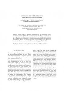
consistency in Section III-E) that are not ω-regular, but can be expressed and verified (both formally and by simulation) using LOC. III. P RELIMINARIES A. Metropolis Meta-Model Metropolis Meta-Model (MMM) is the specification language used in Metropolis design environment. In MMM, the system behavior is specified by three types of objects: processes, media and quantities. Figure 1 shows an example with two producer processes communicating with one consumer model through a medium. A Process has a single active thread. Inside a thread, the code is executed sequentially. Different processes run asynchronously, which is a source of non-determinism. Processes can have ports. The type of a port is an interface defining a set of functions. Through a port, only those functions defined in the same (or sub-) type of port can be called. Media are passive objects. Their methods get executed only when they are called by processes through ports. Quantities are used to model system performance, such as time or power. Though it is also often used to specify scheduling policies, such as first-come-first-serve and time slicing [17], we won’t discuss that aspect in this paper because it is not closely related to the topic of this paper. To understand the following contents, readers can understand a quantity as an object which during execution will annotate performance numbers to events. B. Actions and Events Actions and events are introduced into MMM to define formal execution semantics and to specify formal constraints. Actions include statements and function calls. For instance, in Figure 1, x=R.read(), R.read(), z=foo(x) and W.write(z) are all actions. Each action has two events associated with it, the beginning of the action and the end of the action. For example, W.write(z) is calling the interface function write() defined in medium M. It generates two events beg(P0, M.write)

and end(P0, M.write). P0 indicates the process, which triggers this event; M indicates where the event is physically located. C. LTL in MMM In MMM, LTL can be used to specify coordination among processes. To do that, an LTL formula is defined over events connected with the standard temporal operators • • • •

F f: f G f: f X f: f f U g:

must hold somewhere in the future must hold globally must hold at the next step f must always hold until g holds

or of the form expressed with regular boolean operators •

f , !f , f &&g, f ||g, f → g, f ⇔ g

where f and g are events, or simpler LTL formulas. We can use LTL to specify many meaningful constraints. For instance, in the example shown in figure 1, we want two producers P0 and P1 to write into medium M in a mutual exclusive manner. This can be done by adding the following constraints, which says whenever P0 starts to write, P1 must wait until P0 finishes its writing and vice versa.

E. Expressiveness of LTL and LOC Through several examples and claims, we will conclude that LOC and LTL are incomparable and have different domains of expressiveness. Claim 1: There are LOC formulas that can be expressed with LTL. Since both LOC and LTL contain basic Boolean expressions, a subset of LOC constraints that specify simple global Boolean conditions can be expressed in LTL also. Claim 2: There are LOC formulas that cannot be expressed with LTL. Many quantitative constraints that can be easily expressed by LOC are not suitable for LTL. Specifically, when more than one events need to be compared in the same constraint (e.g. the latency constraint), LTL is not expressive enough to be used. For example, the data consistency constraint: data(input[i]) = data(output[i]) .

(2)

requires comparing the instance of output to input with the same instance index. However, the number of input instances that may occur before the n-th instance of output is arbitrarily large. Therefore, this constraint cannot be modeled by a finitestate system, and it is impossible to express it using any G(beg(P 0, M.write) →!beg(P 1, M.write) U end(P 0, M.write) && formalism based on ω-regular languages, such as LTL or PSL. beg(P 1, M.write) →!beg(P 0, M.write) U end(P 1, M.write)) Claim 3: LOC can express only safety properties. It is well known that safety properties are those which can always be shown violated by a finite trace. Indeed, if a trace D. LOC in MMM does not satisfy an LOC formula, then there must exist an LOC is a formalism designed to reason about traces from the i for which the formula is false. We can evaluate all index execution of a system. It consists of all the terms and operators expressions for that value of i. Since there can only be finitely allowed in sentential logic, with additions that make it possible many of these expressions, there must exist some point in the to specify system level quantitative functional and performance execution such that, for that particular i, the formula does not constraints without compromising the ease of analysis. The refer to any event occurrence beyond that point. Clearly, the basic blocks of LOC formulas are execution prefix up to that point is sufficient to disprove the property. On the other hand, LTL is capable of expressing • constants, or some liveness properties, for example GF (A), i.e. “A occurs • integer variable i (the only index variable that can appear infinitely often”. in an LOC formula), or Conclusion: LOC and LTL are incomparable. • expressions of the form a(e[n]), where a is an annotation Generally, LOC is designed for the specification of quantiname (quantity or data value), e is an event name, and tative performance and functional constraints at the transaction index expression n is an integer-value term, or level where system events and their annotations are considered. • combination of simpler terms using operators. Because of the use of index variable i, LOC is beyond the We interpret a(e[n]) as the value of annotation a of the n-th finite automata domain. On the other hand, LTL is suitable for occurrence of event e. All other terms are interpreted naturally. the specification of functional constraints, and can effectively Terms can be combined using relational operators to create express the temporal patterns for system state transitions. atomic LOC formulas. Finally, LOC formulas are standard Boolean expressions over atomic formulas. IV. S IMULATION AND V ERIFICATION T ECHNIQUES FOR LTL AND LOC C ONSTRAINTS Models of LOC formulas contain a sequence of occurrences for each event name in the formula. We call such structures As discussed in introduction, both LTL and LOC constraints annotated behaviors. Each occurrence may be annotated with can be used as a part of implementation or specification. some quantity annotation, e.g. time, power, etc. Given an As specification, LTL properties can be checked by on/offannotated behavior, we evaluate the formula for each value line simulation or by formal verification. These techniques of index variable i. For example, rate constraint “Display’s are well understood and quite standard, therefore we are not are produced every 10 time units” can be expressed as going to discuss them in this paper. Instead, we will describe simulation based LOC property checking in details, and briefly t(Display[i + 1]) − t(Display[i]) = 10 (1) discuss formal verification of a subset of LOC properties. As

Choose the best transitions* by checking BA

Move forward till next event

Initial state of both system and BA

!" !# $% " # & " # & ' (

Fig. 2.

A Sample B¨uchi Automaton

Eliminate transitions disallowed by BA

Get possible transitions due to system states

*: Maximize the number of runnable events in the system Minimize the distance to an accepting state in BA

Fig. 3.

implementation, the enforcement of LTL constraints and a subset of LOC constraints in simulation is more interesting and will be presented in the following. A. Enforcing LTL Constraints in Simulation A system is specified with the mixture of imperative MMM code and declarative LTL constraints. The task of the simulator is to exhibit the behavior that: 1) can be generated by the imperative MMM code; 2) satisfies the LTL constraints. How to satisfy the first condition efficiently is presented in [18][19]. However, it is difficult to deal with LTL constraints in simulation, because they specify only what the behavior should be, instead of how to realize it. To handle LTL constraints more easily, we choose B¨uchi Automaton (BA) to represent LTL constraints. LTL-to-B¨uchi translation is a well-studied topic in formal verification domain [20], and we have integrated an existing translation tool [21] into Metropolis simulator. 1) B¨uchi Automaton: Figure 2 shows a sample BA, which represents the LTL property that as soon as process P triggers the request event, process C starts to serve and eventually finishes serving. As the figure illustrates, BAs have finitely many states, some of which are designated as initial states or accepting states. States are connected with transitions, and transitions are labeled with enabling conditions. Since an LTL formula refers to events, enabling conditions in the corresponding BAs express possible event schedulings. For instance, the enabling condition tb on the transition from state S3 to S4 denotes that t should not occur, b should occur, while e is don’t-care. A run of a BA is a sequence of states starting from the initial state; between every two adjacent states, the enabling condition must hold. A run of a BA is accepting if it visits some accepting states infinitely often. 2) Simulation Flow and The Use of B¨uchi Automaton: Figure 3 shows the high-level simulation flow. Once the simulator starts from the initial states, the simulator needs to keep track of two sets of states, the system states of all MMM processes and the BA states. When all processes hit some events, event schedulings begins. The simulator must eliminate all illegal transitions in BA first, e.g. the transition with an enabling condition tb is eliminated if b has not come yet. In remaining legal transitions, compatible sets are chosen due to system state and MMM semantics, which must enable at least one transition in the BA if at least one event occurs in

Simulation Flow

LTL constraints1 . At this point, the enabling conditions give all possible event schedulings. Then, check BA again to select the best choice, such as maximizing the number of runnable events. Note that since the BA could be non-deterministic, which is usually the case in our implementation, the simulator needs to do on-the-fly subset construction to maintain a set of, instead of one, current states of the BA. 3) Assisting Heuristics: Since LTL enforcement is done at runtime, no global information is available like in formal verification. This brings in an valid question: which scheduling is the best scheduling in terms of demonstrating the accepting behavior efficiently without expensive look-ahead or backtrack? To partially answer this question, we develop heuristics that attempt to maximize the likelihood that the choice made can be extended into an accepting behavior. Based on our experiments, the heuristics works very well on typical coordination constraints expressed by LTL. The first heuristic is to maximize the number of events that can run, e.g. event b in tb transition and the donot care event e if possible. This will prevents a process from idling at a state and let the system proceed as quickly as possible, therefore minimize the total simulation time. The second one is to minimize the distance to accepting states in BA. This tries to lead the system to demonstrate accepting behavior specified by LTL constraints. To realize the second heuristic, we first annotate each state in BA with an integer number before simulation, which indicates the minimum number of steps in which it can reach an accepting state. This could be easily done by backward traversal of the BA. Then during simulation, whenever there are multiple choices, always choose the next state in BA which has the minimum step number. If on-the-fly subset construction is needed, take the minimum minimum-step-numbers among all the states in the subset. B. Enforcing Built-in LOC Constraints in Simulation General LOC constraints are usually difficult to understand, not to mention enforcing them effectively in simulation. However, designers are familiar with a subset of LOC constraints, 1 The simulator should just check the BA for the events appearing in LTL constraints. If no events present in the current system state, no action is needed on the BA side.

which are quite often used in real world designs. So, we provide these constraints as a set of built-in LOC constraints(BIL), including maximum rate, minimum rate, maximum latency, minimum latency, and period. To enforce BILs, we need to integrate them into time quantity. The entire simulation process consists of parsing the BIL, registering BIL to time quantity, resolving BIL, and annotating quantity. For example, we add a maximum latency BIL of 10 clock cycles on an event. After parsing and registering it to time quantity, in simulation whenever time needs to be advanced, time quantity will check whether the last occurrence of that event would be 10 clock cycles before the new time, had time been moved forward. If that is the case, in order not to violate the BIL, time quantity will prevent time from advancing until that event comes. As soon as it comes, time quantity will annotate a proper value to it. Other BILs can be handled in similar ways. C. Simulation Trace Checker for LOC In simulation verification, we automatically generate simulation trace checkers from LOC formulas. In the LOC checker, we use a linear-time algorithm to check the simulation trace, which could be infinite, and see if an LOC formula can be satisfied for all possible values of index i. Although the algorithm is linear in time, memory space usage is dependent on the formula heavily. To reduce the running time, we try to scan the whole trace only once and store the annotation information that is expected to be useful in the future. Therefore, a memory recycling procedure has to be invoked frequently to release unnecessary memory space to obtain space efficiency. The algorithm of LOC checking progresses based on the index variable i. Each LOC formula instance is checked sequentially with the value of i being 1, 2, ..., etc. [6] The time complexity of the algorithm is linear in the size of the trace since evaluating a particular Boolean expression takes constant time. The memory usage, however, may become prohibitively high if we try to keep the entire trace in the queue for analysis. As the trace file is scanned in, the checker attempts to store only the useful annotations, and in addition, to evaluate as many formula instances as possible, and to remove from the memory parts of the annotations that are no longer needed (memory recycling).

figure out whether the design needs to be altered. If the verification session runs too long, approximate verification can be used to explore a subset of the state space and report the probability that the property will pass. Obviously, a partial exploration cannot prove that a property holds. However, it is our experience that a lot of “easy” bugs can be found within a relatively small amount of time and memory usage. If a Spin verification session continues to run after a long time, it is highly likely that the property will eventually pass. V. C ASE S TUDY — F UNCTION M ODEL FOR V IDEO P ROCESSING A. Function Model for Video Processing Figure 4(a) shows the block diagram of a Picture-in-Picture (PIP) application. A single input transport stream (TS) is demultiplexed and parsed into multiple MPEG video streams. Controlled by the user’s input, decoded video streams can be resized and fed to JUGGLER which combines them into picture-in-picture videos. In this design, RESIZE is the major component that computes and adjusts the size of MPEG video frames. It consists of about 9,000 lines of Metropolis MetaModel source code and contains 22 concurrent processes and more than 300 communication media. During simulation, a deadlock problem was detected in RESIZE[22], specifically, on the communication among TMEM CTL U, TMEM CTL V and TMUX UV processes. See figure 4(c). The reason is that TMUX UV fails to consume all the data generated by TMEM CTL U and TMEM CTL V. Knowing all above, we can fix the problem by implementing a scheduling policy among the three processes. If written imperatively, this would require adding hand-shaking signals and scheduling algorithm. As an alternative, we can simply constrain the write and read operation with LTL constraints, which is much easier than the first approach. The LTL properties we use are as follows. They are basically saying the read and write operation should alternate. G(writeU → (!F (writeU ) U read) && read → (!F (read) U writeU )) G(writeV → (!F (writeV ) U read) && read → (!F (read) U writeV )) writeU = end(T M EM CT L U, T M EM CT L U.write) writeV = end(T M EM CT L V, T M EM CT L V.write) read = end(T M U X U V, T M U X U V.read))

D. Formal Verification For formal verification in Metropolis, the MMM description is automatically translated into Promela description, and the LTL properties specified in MMM are checked using the model checker SPIN [6]. It is known that only a subset of LOC can be translated into equivalent LTL formulas and formally checked with SPIN directly [4]. For the rest of the LOC formulas, the formal verification results may be inconclusive, i.e. the verification is only partial. The designer may perform any synthesis step (e.g. composition, decomposition, constraint addition, scheduler assignment) and a new Promela code can be automatically generated to verify the property. If it does not pass, the error trace may be used to help designers

The simulation result shows no deadlock after adding above constraints. In order to quantitatively investigate the simulation, we profile the simulation run with LTL constraints enforcement. It shows that the overhead to enforce LTL constraints is 1% of the total simulation time. In the transaction-level design of PIP, where time is still not available, we can check both functional and performance constraints with proper annotations output from the simulation. In the component RESIZE of PIP, the images processed are in interlaced format with alternating fields of all odd lines, then all even. The image size should only change after a complete frame, each of which has 2 fields, is produced. Therefore, the

SVSRC

USRCONTROL

USRCONTROL

Picture−in−Picture RESIZE

MPEG

SHSRC

SVSRC

WINDOW

TMEM_CTL_U

TMEM_CTL_V

TMUX_UV

PES_PARSER

JUGGLER

MPEG TS_DEMUX

RESIZE

(a) Picture-in-Picture Block Diagram

(b) Resize Module Block Diagram Fig. 4.

(c) Details in SVSRC

Picture-in-Picture

field sizes of paired even and odd fields should be the same. This property can be expressed as an LOC formula: size(field start[2i + 2]) − size(field start[2i + 1]) = (3), size(field start[2i + 1]) − size(field start[2i]) where field start is an event at which RESIZE starts to output a new image field. The annotation size is the total number of pixels processed by RESIZE. The generation of the checker for this LOC formula and the actual checking on the simulation trace take less than 1 minute of CPU time. We also check performance properties such as latency. The latency issue in RESIZE relates to the timely response to user size specification. Since PIP is specified at the behavior level, no detail timing information is available. We therefore specifies a bound (e.g. 5) on the number of fields processed between reading a new size specification (read size) and the actual change in output image size (change size): field count(change size[i])−field count(read size[i]) ≤ 5 , (4) where read size is generated whenever RESIZE reads a new size specification from USRCONTROL, and change size is generated whenever the size of the output image is actually changed. The annotation field count is the value of a global counter that is incremented by one whenever RESIZE processes a new image field. The generation of the checker for this LOC formula and the actual trace checking also take less than 1 minute of CPU time. VI. C ONCLUSIONS In this paper, we have presented our constraints assisted design and verification methodologies, where constraints are used to aid system modeling, enforced as a part of system implementation, and checked as a part of system properties. We have introduced the algorithms to enforce LTL and builtin LOC constraints in simulation. We have also introduced the verification techniques integrated in the Metropolis design environment for the properties specified with LTL and LOC. The industrial multimedia application have demonstrated the effectiveness of modeling with constraints and the efficiency of our simulation tool and simulation trace checker. R EFERENCES [1] F. Balarin, Y. Watanabe, et al.: Metropolis: An Integrated Environment for Electronic System Design. IEEE Computer Society, April, 2003

[2] K. Keutzer, S. Malik, R. Newton, J. Rabaey, A. Sangiovanni-Vincentelli: System Level Design: Orthogonalization of Concerns and Platform-Based Design. IEEE Transactions on Computer-Aided Design of Circuits and Systems, Vol. 19, No. 12, Dec. 2000 [3] A. Pnueli: The Temporal Logic of Programs. Proceedings of the 18th IEEE Symposium on Foundation of Computer Science, 46-57, 1977 [4] X. Chen, H. Hsieh, F. Balarin, Y. Watanabe: Logic of Constraints: A Quantitative Performance and Functional Constraint Formalism. IEEE Transactions on Computer-Aided Design of Integrated Circuits. Vol. 23, No. 8, Aug. 2004. [5] Gerard J. Holzmann: The Model Checker SPIN. Software Engineering, 279-295, Vol. 23, No. 5, 1997 [6] X. Chen, H. Hsieh, F. Balarin, and Y. Watanabe: Formal Verification for Embedded System Designs. International Journal of Design Automation for Embedded Systems. Special Issue of Covalidation of Embedded Hardware/Software System, edited by Ian G. Harris. Kluwer Academic Publishers, 8(2/3), June/September 2003. [7] P. Alexander, C. Kong, D. Barton: Rosetta usage guide. available at http://www.sldl.org 2001 [8] Accellera: http://www.accellera.org [9] IBM: http://www.haifa.il.ibm.com/projects/verification/sugar [10] OpenVera: http://www.open-vera.com [11] Object Constraint Language specification. http://www. omg.org, 1997. [12] Quick reference guide for the Design Constraints Description Language. http://www.eda.org/dcwg, 2000. [13] F. Jahanian, A. K. Mok: Safety Analysis of Timing Properties in RealTime Systems. IEEE Transactions on Software Engineering, 890-904, 1986 [14] B. Alpern, F. Schneider: Verifying temporal properties without temporal logic. ACM Transactions on Programming Languages, vol 11, no 1, 147167, Jan 1989 [15] Z. Har’El, R. P. Kurshan: Software for Analysis of Coordination. Proceedings of the International Conference on System Science, 382-385, 1988 [16] J.G. Henriksen, J. Jensen, et al: Tools and Algorithms for the Construction and Analysis of Systems. Mona: Monadic Second-order logic in practice First International Workshop, TACAS ’95, LNCS 1019 [17] V. Shah, C. Passerone, L. Lavagno, Y. Watanabe: A time slice based scheduler model for system level design. Design Automation and Test in Europe, page 378, 2005. [18] F. Balarin, L. Lavagno, et al.: Concurrent Execution Semantics and Sequential Simulation Algorithms for the Metropolis Metamodel. Proc. 10th Int’l Symp. Hardware/Software Codesign, 13-18, 2002 [19] G. Yang, Y. Watanabe, F. Balarin, A. Sangiovanni-Vincentelli: Separation of Concerns: Overhead in Modeling and Efficient Simulation Techniques. Fourth ACM International Conference on Embedded Software (EMSOFT’04), Sep. 2004 [20] Fabio Somenzi and Roderick Bloem: Efficient Buchi Automata from LTL formulae. [21] Paul Gastin and Denis Oddoux: Fast LTL to Buchi Automata Translation. CAV, 2001 [22] X. Chen, A. Davare, H. Hsieh, A. Sangiovanni-Vincentelli, Y. Watanabe: Simulation based deadlock analysis for system level designs. DAC ’05: Proceedings of the 42nd annual conference on Design automation, 260265, 2005