MODELING AND VALIDATION OF A GREENHOUSE CLIMATE MODEL Javier Leal Iga ∗ Efra´ın Alcorta Garc´ıa ∗ Humberto Rodr´ıguez Fuentes ∗∗ ∗
Facultad de Ing. Mec´ anica y El´ectrica, UANL, MEXICO ∗∗ Facultad de Agronom´ıa, UANL, MEXICO
[email protected];
[email protected];
[email protected]
Abstract. In this work it is proposed an extension to the Greenhouse climate model given by (Tap, 2000). The extension considers the effect of humidity in the air temperature as well as some terms related to the use of fogs, shade cloth and fan. The introduced modification is validated using measurements of a greenhouse in north west Mexico. The results show that the proposed model is adequate to c simulate the climate behavior of the Greenhouse. Copyright ° 2005 IFAC Key Words. Nonlinear systems, Greenhouse climate, modeling, validation.
1. INTRODUCTION The main purpose of a greenhouse is to improve the environmental conditions in which plants grown. Greenhouse climate is influenced by many factors, for example, by outside temperature, wind, humidity, the crop, etc. Many dynamic climate models of a greenhouse have been proposed in the last 25 years. Basically, these models are based on mass and energy balances. In 1983 some simple models were proposed. These models include a first order linear approximation with empirical crop models (Udink ten Cate, 1983) and a nonlinear high order model, without the crop consideration and the requirement of the sky temperature (Bot, 1983). After these seminal work, many enforce has been done in order to get more useful models. In (Tchamitchian, 1993) proposes a 3rd nonlinear model which includes a simple model of a crop. Independent of early approaches Takakura (Takakura, 1993) proposes a nonlinear model which considers a cover temperature, inside air temperature, floor and plant temper-
ature. From other point of view (Nielsen and Madsen, 1998) proposes a linear continuous time stochastic model. Other approach has been considered in (Ferreira and Ruano, 2002) where a neural network based model of the climate of a Greenhouse has been explored. A more complete climate model has been proposed in (Tap, 2000), which considers a 4th order nonlinear model. A differential equation to the humidity was incorporated to the climate model and the effect of transpiration and respiration of the crop, condensation as well as a better calculation of the air flow in the Greenhouse were also considered. In this work is proposed a greenhouse climate model extension. Basically, the effect of the humidity on the air temperature as well as the effect of fans, shade cloth and fogs are added. For validation, measurement of meteorological variables of a greenhouse located in north west Mexico are taken. The results show that the proposed modifications are useful to model the greenhouse climate.
The work it is organized as follows. In section 2 a climate model of the considered Greenhouse is presented. In section 3 measured data and parameters used for validation are exposed. A comparison between measurements taken inside of the greenhouse and the obtained from the proposed model is shown in section 4. In section 5 some conclusions are discussed.
s = s1 Tg2 + s2 Tg + s3 g = g1 (1 − g2 e−g3 G )e−g4 Ci λ = L1 − L2Tg ½ m m1 (W g − Wc∗ ) |Tg − Tc | 2 Wg > Wc∗ Mc = 0 Wg ≤ Wc∗ ∗ ωPc Wc∗ = Patm − Pc∗ a2 Tc
2. GREENHOUSE CLIMATE MODEL As mentioned above, the start point for this work is the model given by (Tap, 2000). This consists basically in four nonlinear differential equations for the state variables: air temperature Tg (t), soil temperature Ts (t), humidity Vi (t) and CO2 concentration represented by Ci (t). Note that the description of all variables of the equations can be found in the Appendix A. The model equations are the follows: Greenhouse air temperature The following equation results of consider the temperature equation from (Tap, 2000) and added the effects of: a) Air density variation due to d humidity dt (Cg Tg ) with Cg = h(cp γ0 + CH Vi ) time variant (Leal, et. al., 2004) [show in bold on equation (1) and (4)]; b)The effect of fans [φf an on equation (3), apply directly as the flow adding for fans ]; c) Shade cloth [Z on equation (1), as percent reduction of incoming radiation ]; d) And fogs [Q on equation (1), (2) and (7), directly calculated with the amount of humidity adding for fogs (Qf )]. dTg 1 = [Kv (To − Tg )+ (1) dt h(cp γo + CH Vi ) +α(Tp − Tg ) + Kr (To − Tg ) + λMc Ks (Ts − Tg ) + ZηG − λE + − ²+1 CH Tg (E − φv (Vi − Vo ) − Mc + Q)] where:
Pc∗ = a1 e a3 +Tc ² 1 Tc = To + Tg ²+1 ² ωPg Wg = Patm − Pg Pg = Λ(Tg + To )Vi Note that the air temperature equation of (Tap, 2000) considers the heat exchanges between: Greenhouse indoor and outdoor air, Greenhouse indoor air and pipe heating system, Greenhouse indoor air and the roof, Greenhouse soil and indoor air, as well as the influence of: solar radiation, heat loss for evaporation due transpiration, heat input due condensation of water vapor on the roof and a tomato crop. Greenhouse soil temperature Cs
ρ · Qf Ag φv = φvent + φf an Kv = (γo + Vi )cp φv σrwl φvent = ( + ζ + ξrww )W + ψ 1 + χrwl qSnηG + rρcp Dg gb E = WL λ(S + γ(1 + ggb ) a2 T g
Dg = a1 e a3 +Tg − Λ(Tg + To )Vi
(2) (3) (4)
(5)
The soil differential equation considers the heat exchange between the Greenhouse indoor air and the soil ground and the heat exchange between the superficial and the deep soil. Greenhouse CO2 concentration Vg dCi = φv (Co − Ci ) + ϕinj + R − P Ag dt where R=
MCO2 MCH2 O
(Tg −20) 10
Q10
(6)
ρr Wm
"
Pmax = τc Ci Teff
P =
Q=
dTs = −Ks (Ts − Tg ) + Kd (Td − Ts ) dt
Pmax Log K
# 1−
h
p
(Tg − Tmin )(Tg − Tmax ) (Tg − Tmin )2 (Tg − Tmax )2 + Tcs
(1 − m)Pmax + ∈p Kp I
i
(1 − m)Pmax + ∈p Kp Ie−Kp ·LAI
The CO2 concentration differential equation is formed by mass balance between CO2 indoor and outdoor; CO2 injection flux; crop photosynthesis and CO2 contributed by respiration. Greenhouse air water vapor concentration Vg dVi = E − φv (Vi − Vo ) − Mc + Q (7) Ag dt The water vapor concentration consider the effect of transpiration mass balance between transpiration crop, indoor and outdoor humidity, minus
cover condensation, and plus humidity add for nebulizators.
the lee, windward and upper windows are open at 100 % for operation almost all part of day. A tomato crop is in the Greenhouse.
3. MODEL VALIDATION
In this work, some signals were taken manually because of the impossibility to record them automatically. The signals under this situation are: the time at switch on and off of fogs; measurement in place of CO2 (in this study are used a vector of estimated data based in measurements of other similar studies); opening of windows in rainy nights; the humidity amounts added at ambient into greenhouse (sometimes the operator of greenhouse spray water directly on crop, with intention of reduce the air temperature). All of these were measured in situ during day time, but at night was impossible and were approximated with the information of operators.
The validation is concerned with determining whether the proposed model is adequate or not. In this section it is presented a way to verify the pertinence of the proposed model as well as the condition under the test is carried out. 3.1 Validation process The verification of the proposed model is realized based on physical measurements of a Greenhouse, see figure 1, which is located in north-west Mexico. The idea is to obtain measurements of the input and output signals of the Greenhouse. In order to use the proposed model to generate an estimated output and compare it with the measured output. Two sets of data are considered: Case A: 5 days, with fogs switch on/off. Case B: 14 days, with fogs switch off. The measurement signals with data acquisition
3.3 Measured data The measurements obtained from the data acquisition outdoor of the greenhouse are shown in figure 2 for Case A, and figure 3 for Case B. Outdoor Temperature 40 35 °C
Kg/m3
0.02
30
0.015
25 20
Outdoor Absolute Humidity 0.025
0
2
4
6
0.01
0
2
4
6
Solar Radiation 6
400
4
200
Figure 1. Greenhouse used for the experiments equipment were air temperature, relative humidity, solar radiation, wind speed, atmospheric pressure, greenhouse outdoor, and air temperature and relative humidity at greenhouse indoor. Note that for the soil temperature and the deep soil temperature only pointing measurements has been utilized. From the above signals only the air temperature inside of the Greenhouse and the relative humidity in the Greenhouse are considered as outputs. The rest of the signals are used together with the model to estimate the outputs. 3.2 Experiment conditions The greenhouse is equipped with 4 fogs and 4 fans on north wall, the air is continuously renewed during day and night. Moreover, in this greenhouse
0
Wind Speed
m/s
W/m2
600
2
0
2
4
6
0
0
Days.
2
Days.
4
6
Figure 2. Outdoor data: Case A The record operation of fogs is presented in figure 4. This information will be used in Case A. All other values for variables and parameters are specified in Appendix A. It is important to note that all the values of parameters correspond to the physical sense, none of them has been modified for calibration or some other reason.
4. EXPERIMENTAL RESULTS With the measurements available the simulation for the different cases were developed.
Kg/m3
°C
20
0.02
0.015 0
5
10
15
0.01
0.03 0.028
Absolute Humidity Kg/m3
0.025
30
10
0.032
Outdoor Absolute Humidity 0.03
Outdoor Temperature 40
0
5
Solar Radiation
10
0.026 0.024 0.022 0.02 0.018
15
0.016 0.014
Wind Speed 6
400
4
200
0
1
2
3 Days.
4
5
6
Figure 6. Greenhouse absolute humidity. The continuous line represent the measurements and the dash line the simulation
m/s
W/m2
600
2
12
0
5
10
0
15
0
5
Days.
10
15
8
Figure 3. Outdoor data: Case B −3
1.2
10
Days.
Temperature °C
0
x 10
6 4 2 0
−2 −4
1
Humidity Kg/m3
−6 −8
0.8
0
1
2
3 Days.
4
5
6
0.6
Figure 7. Greenhouse air temperature. Difference between measured and simulation data.
0.4
0.2
0
−3
0
1
2
3 Days.
4
5
x 10
6
6
Figure 4. Indoor humidity add for fogs: case A 4.1 Case A The comparison of measurements in land and results of model, are in figure 5, figure 6:
Absolute Humidity Kg/m3
4 2 0 −2 −4 −6 −8
0
1
2
3 Days.
4
5
6
40 38
Figure 8. Difference between measured Greenhouse humidity and the simulation
36
Temperature °C
34 32
very close. The simulation for the humidity is closer than the one of the temperature, and result with a correlation of 0.6098.
30 28 26 24 22 20
0
1
2
3 Days.
4
5
6
Figure 5. Greenhouse air temperature. The continuous line shows the measurements and the dash line represents the simulation model
4.2 Case B The comparison are in figure 9, figure 10: 40
35
Temperature °C
In the figure 5, it can be seen that the output obtained by simulation is very similar to the measurement. There are some differences, however them can be considered acceptable. Figure 7 shows the difference between real and simulated greenhouse air temperature. The mean value resulting is 2.4 ◦ C, the variance of 5.87 and the correlation between simulated and measured was 0.9534. In the same case, the figure 6 shows the measured greenhouse humidity against the simulation. The most important differences are present in half day, in the rest of day the similitude are
30
25
20
15
0
2
4
6
8
10
12
14
Days.
Figure 9. Greenhouse air temperature. The continuous line show the measurements and the dash line represent the simulation model
or parameter, the result must improve with more time and resources let adjust this values.
0.035
Absolute Humidity Kg/m3
0.03
0.025
5. CONCLUSIONS
0.02
0.015
0.01
0
2
4
6
8
10
12
14
Days.
Figure 10. Greenhouse absolute humidity. The continuous line represent the measurements and the dash line the simulation In the figure 9, we can see like the prognostic model are more close at real measurements than figure 5, the effect of fogs switch off improve the results. And in the figure 11, which show the differential between real minus simulated greenhouse temperature, resulting with a mean of 1.06 ◦ C, variance of 2.50 and correlation of 0.98. 10 8
Temperature °C
6 4 2 0
−2 −4 −6 −8
0
2
4
6
8
10
12
14
Days.
Figure 11. Greenhouse air temperature. Difference between measured and simulation For the humidity, the figure 10 shows greenhouse humidity real against simulated with the proposed model. And as it can be seen, the results model present good behavior with a correlation of 0.8093, and required more adjust for calibrate better the model at conditions of greenhouse tacked in this study (like the exact moment in which turn on/off the fogs for operators each day). From this graphic we can see how in the half day the model presents the most important differences, in the rest of day the similitude is very close. It −3
10
x 10
Absolute Humidity Kg/m3
8 6 4 2 0 −2 −4 −6
0
2
4
6
8
10
12
14
Days.
Figure 12. Greenhouse humidity: difference between measured and simulation is important to note the fact that the proposed approach does not change any value for variable
An extension and validation of a climate greenhouse model has been presented. Based on the climate model of (Tap, 2000), and including the modification of (Leal, et. al., 2004) in order to consider the humidity variations in the air temperature equation. Besides the above modification, some terms to consider the effect of fans in walls, fogs and shadow cloth have been included. To test the proposed modifications, a real Greenhouse in north-west Mexico has been used. Measurements of the required variables in real operation were acquired. The measurements of the output variables are compared to the related simulation obtained using the proposed model. Two series of data were utilized to the test. In the first case fogs has been utilized in order to reduce the temperature, Case A. For the second data set, Case B, the fogs were turn off. As can be seen, the results from the figures 5-12 and correlations, shown an acceptable behavior in both cases. Although we found a good behavior with the model, further work should keep on working sampling a greenhouse during all a year, in order to evaluate the model under different weather conditions. And include the design of a control strategy for the temperature variable.
6. ACKNOWLEDGMENTS The authors are gratefully to Ing. Fco. Barrera Cumming, whom give facilities to do the study.
REFERENCES Bot, G. (1983). Greenhouse Climate: from physical processes to a dynamic model, PhD Thesis. Wageningen Agricultural University. Institute of Agricultural and Environmental Engineering and Physics The Netherlands., P.O.B. 43,NL-6700 AA Wageningen Uni. Ferreira, P. M. and A. E. Ruano (2002). Choice of rbf structure fpr predicting greenhouse inside air temperature. In: IFAC 15th World congress. Barcelona. Leal Iga, J., Alcorta Garc´ıa, E. and Rodr´ıguez Fuentes, H. (2004). Influence of air density variations in the climate of a greenhouse. In: 2nd IFAC symposium on system structure and control. Oaxaca, Mexico. Nielsen, B. and H. Madsen (1998). Identification of a linear continuous time stochastic model of the heat dynamic of a greenhouse. J. Agr. Eng. Res. 71, 249–256.
Takakura, T. (1993). Climate under cover, digital dynamic simulation in plant Bioengineering. Kluwer Academic Pub. The Netherlands. Tap, F. (2000). Economics-based optimal control of greenhouse tomato crop production, PhD Thesis. Wageningen Agricultural University. Institute of Agricultural and Environmental Engineering and Physics The Netherlands., P.O.B. 43,NL-6700 AA Wageningen Uni. Tchamitchian, M. (1993). Optimal control applied to tomato crop production in a greenhouse. In: European Control Conference. Groningen. Udink ten Cate, A. J. (1983). Modeling and (adaptive) control of greenhouse climates, PhD Thesis. Wageningen Agricultural University. Institute of Agricultural and Environmental Engineering and Physics The Netherlands., P.O.B. 43, NL-6700.
(3) Ks
= 5.75 = 0.7 (3) Kd = 2 (1) α = 0 (1) Z = 0.6 (1) Td = 19 (1) Vg = 4555.4 (1) Ag = 1050 (1) ϕinj = 0 (1) rw l = 100 (1) rw w = 100 (1) WL = 75 (3) LAI = 3 (2) η
(3) Wm
(2) Mair
= 0.17 = 1.29 (2) γo = 1.205 (2) ρ = 998 (2) Patm = 101.0 (3) ω = 0.622
Kg Dry air density at 0 ◦ C, m 3 Kg Dry air density at 20 ◦ C, m 3 Kg Specific mass of water, m 3 Atmospheric air pressure, kP a Humidity ratio
(3) q
Evaporation radiation,
= 0.01
Functions Q Dg s g Wc∗ Pc∗ Tc Wg Pg λ
Kg Humidity add for fogs s·m2 Air vapor pressure deficit, kPa a Saturated water vapor-pressure slope, kP ◦C Leaf conductance Humidity ratio at sat. cover vapor pressure Saturated vapor pressure at cover Cover temperature Greenhouse air humidity ratio Greenhouse air vapor pressure Vaporization energy of water, Joules g
Kv E Mc
Ventilation heat transfer coeff., g Crop transpiration rate, s·m2 Condensation water flow, mg2 s
R P φv φvent
W
m2
◦ C·
g CO2 Crop respiration, s·m 2 g CO2 Crop photosynthesis, s·m 2 m Ventilation flux, s m Ventilation flux for windows, s
Inputs To Tp G Co Vo W Qf
Outside air temperature, ◦ C Heating pipe temperature, ◦ C Short-wave radiation, watts·m−2 Outside air CO2 concentration, mg3 Kg Outside water vapor concent., m3 Wind speed m s 3 Water consuming for fogs, ms
System states Tg Ts Ci Vi
Greenhouse air temperature, ◦ C Greenhouse soil temperature, ◦ C Greenhouse CO2 concent., mg3 Kg Greenhouse water vapor concent., m3
Parameters (1) φf an
= 11.4 (2) cp = 1010 (2) Cs = 120000 (2) Ch = 2010 (1) Kr = 0.3349
Ventilation flux for fans, m s Jouls Air specific heat, Kg· ◦C Jouls Greenhouse soil heat cap., Kg· ◦C Jouls Water vapor specific heat, Kg· ◦C W Roof heat transfer, ◦ C· m2
m2
m2 g
2
= 0.01 (3) n = 0.098 (3) gb = 10 (3) γ = 0.067 (3) ² = 3 (3) s1 = 0.00018407 (3) s2 = 0.00097838 (3) s3 = 0.051492 (2) Λ = 0.46152 (3) a1 = 0.611 (3) a2 = 17.27 (3) a3 = 239 (3) ζ = 0.000027060 (3) σ = 0.000071708 (3) χ = 0.0156 (3) ξ = 0.000063233 (3) ψ = 0.000074 (2) L1 = 2501 (2) L2 = 2.381 (3) g1 = 20.3 (3) g2 = 0.44
Ev. vapor pressure deficit, mg Parameter of radiation Boundary layer conductance, mm s a apparent psychometric constant, kP ◦C Inside outside cover heat resistance. a Sat. water vapor press. par. 1, kP ◦C3 kP a Sat. water vapor press. par. 2, ◦ C 2 a Sat. water vapor press. par. 3, kP ◦C m Pressure constant, N ◦C g Saturation vapor pressure, kP a Saturation vapor pressure Saturation vapor pressure, ◦ C Renewal rate parameter, m s Renewal rate parameter Renewal rate parameter Renewal rate parameter Renewal rate parameter Vaporization energy coefficient, Jg Vaporization energy coefficient, g J◦ C Leaf conductance, mm s Leaf conductance
(3) g3
Leaf conductance,
(3) r
APPENDIX A: STATES, INPUTS, FUNCTIONS AND PARAMETERS
W Soil heat transfer, ◦ C· m2 Radiation conv. factor W Soil to soil heat transfer, ◦ C· m2 W Pipe air heat transfer, ◦ C· m2 Effective solar radiation Deep soil temperature, ◦ C Greenhouse volume, m3 Greenhouse surface, m2 g CO2 Injection flux, s·m 2 Rel. lee window opening Rel. windward window opening Leaf dry weight, mg2 Crop leaf area index Crop dry weight, KgCH2 O
= 0.0025
(3) g4
= 0.00031 = 0.0010183 (3) m2 = 0.33 (4) MCO2 = 0.044 (4) MCH2 O = 0.03 10 = 1.40 (4) Q
s m2 µmol m3 g
(4) ρr
Leaf conductance, g Mass transfer, s m 2 Mass transfer Kg Carbon dioxide molar mass, mol Kg Glucide unit molar mass, mol Respiration of the crop Maintenance respiration, KgCH2 0
2.46×10⁻⁹ m = 0.10 (4)
Leaf transmission factor
(3) m1
= 1.2 × 10⁻⁷ (4) τc = 0.0029 (4) Tef f = 0.54 (4) Kp = 0.58 (4) Tmin = 7 (4) Tmax = 38.5 (4) Tcs = 19840 (4) ∈p = (2) Qf
= 0.0011
Kg·s
Leaf CO2 efficiency, m s Amplitude of temp effect, ◦1C Crop light extinction coefficient Min. temp for photosynthesis, ◦ C Max. temp for photosynthesis, ◦ C Smoothness for temp effect, ◦ C 2 Quantum yield efficiency, KgCO2 µmol
Fog water consumption
m3 s
measured in situ, or property obtained for the materials used in greenhouse. (2) values taken from his physics property. (3) Obtained from (Tap, 2000). (4) Obtained from (Tchamitchian, 1993). (1)