Constructive density estimation network based on several different separable transfer functions. WÅodzisÅaw Duch and RafaÅ Adamczak. Department of ...
ESANN'2001 proceedings - European Symposium on Artificial Neural Networks Bruges (Belgium), 25-27 April 2001, D-Facto public., ISBN 2-930307-01-3, pp. 107-112
Constructive density estimation network based on several different separable transfer functions. Włodzisław Duch and Rafał Adamczak Department of Computer Methods, Nicholas Copernicus University, Grudzi¸adzka 5, 87-100 Toru n´ , Poland. http://www.phys.uni.torun.pl/kmk Geerd H.F. Diercksen Max-Planck Institute of Astrophysics, 85740-Garching, Germany Abstract. Networks estimating probability density are usually based on radial basis function of the same type. Feature Space Mapping constructive network based on separable functions, optimizing type of the function that is added, is described. Small networks of such type may discover accurate representations of data. Numerical experiments on artificial and real datasets are reported.
1
Introduction
Neural networks based on sigmoidal, radial and many other types of transfer functions, are universal approximators [1]. Unfortunately there is no guarantee that such networks will find a good solution. Approximation of complex decision borders by a neural network requires flexibility that is usually provided only by networks with sufficiently large number of parameters. Despite regularization techniques which help to avoid overparameterization training of such networks may be difficult and prone to the local minima problems. It is commonly believed that learning and architectures are the most important issues in neural computing. One relatively unexplored way to improve the performance of neural networks in complex problems is to optimize transfer functions performed by artificial neurons. The situation is analogous to the “nature” versus “nurture” debate: although MLP networks may in principle learn all kinds of data the inner ability of a network to learn quickly requires flexible “brain modules”, or transfer functions that are appropriate for the problem to be solved. It is easy to construct N-dimensional training data that can be handled correctly by a single hyperplane (suitable for MLPs with complexity O(N)) or by a spherical, localized functions (suitable for RBF networks with Gaussian functions and O(N) complexity). Inappropriate model applied to such data will need at least O(N 2 ) parameters, making the training process harder. Rates of convergence and complexity of models necessary to approximate or classify data depends strongly on the type of transfer functions used. A survey of transfer functions suitable for neural networks The authors acknowledge POL-040-98 grant for German-Polish collaboration. W.D. is also grateful for support by the Polish Committee for Scientific Research, grant 8 T11C 006 19.
ESANN'2001 proceedings - European Symposium on Artificial Neural Networks Bruges (Belgium), 25-27 April 2001, D-Facto public., ISBN 2-930307-01-3, pp. 107-112
has been presented in [6], and a taxonomy of such functions in [7]. Constructive algorithms that add one transfer function at a time are very attractive but so far have been restricted to functions of the same type. Models that select or optimize the type of function that is added have not been used so far. Feature Space Mapping (FSM) neural model [2] is based on multidimensional separable transfer functions. Such choice of transfer functions has some advantages over the radial basis functions [1]. A separable transfer function f (X) = ∏Ni=1 fi (Xi ) may be interpreted as a conjunction of fuzzy membership functions f i (Xi ). Viewed from various perspectives FSM is a neurofuzzy system, a probability density estimation network modeling p(X|C i ), localized transfer functions enable a memory-based interpretation (generalization of the training data to form reference prototype vectors), and the unsupervised training leads to a self-organizing system that models distribution of data using prototypes. The main idea is simple: components of the input vectors X i and the output vectors Yi define features, and probability distributions in the feature spaces define fuzzy prototypes or memorized “objects”. These objects are described by the joint probability density of the input/output data vectors p(X,Y |M) using a network M based on some transfer functions. Although this model may be presented in probabilistic framework as a density network it was originally inspired by cognitive model of mind as an approximation to real neurodynamics – high activity of the spiking neurons may be described by the probability density function in the feature space [3]. The importance of density estimation as the basis for neural systems has recently been stressed by many authors (cf. [1]). FSM model has been implemented as a constructive network using several types of transfer functions: Gaussians, triangular, trapezoidal, rectangular or soft trapezoidal functions (products of pairs σ(X i − b) − σ(Xi + b) of sigmoidal functions). The network has been tested on a number of classification problems and has been used for extraction of fuzzy and crisp logical rules. It may also be used as an associative memory, predicting the values of a part of X vector from any other part. In previous papers general philosophy, the training algorithm, parameterization of rotated bicentral transfer functions and initialization of neural networks parameters has been described[2, 4, 5]. The FSM model has been extended here to allow for different transfer functions that are added during the process of network growth. After a brief description of the FSM network recent developments are described and issues connected with optimization of transfer functions are discussed. Results of computer experiments are presented in section 3 which is followed by conclusions.
2
FSM model
FSM model as used for classification is described very briefly here. Since training of the MLP networks or other networks with fixed architecture is tedious a robust constructive algorithm is used to build the FSM network. In the simplest case a single hidden layer structure is used. Initial architecture is created using clusterization techniques [5] and optimized during learning process. A set of training examples D = {X k ,Y k } is used to create a network M(X,Y ; P), where P are adaptive parameters of the network that gives outputs approximating the landscape of joint proba-
ESANN'2001 proceedings - European Symposium on Artificial Neural Networks Bruges (Belgium), 25-27 April 2001, D-Facto public., ISBN 2-930307-01-3, pp. 107-112
bility density p(X,Y |D ). The M(X,Y ; P) should be neither equal to, or proportional to, this density; all that is required is that the maxima of conditional probabilities Yp (X) = maxY p(Y |X, D ) and X p (Y ) = maxX p(X|Y, D ) agree with the corresponding maxima of M(X,Y ; P) obtained by calculation of Y M (X) = maxY M(X,Y ; P) and XM (Y ) = maxX M(X,Y ; P). This task is simpler than the full estimation of joint or conditional probabilities. Transfer functions: good transfer functions φ(X; θ) should offer the most flexible densities (flexible shapes of φ(X; θ) =const contours) with the smallest number of adaptive parameters θ. A small network with a few flexible transfer functions is equivalent to a large network with typical sigmoidal or Gaussian nodes. The FSM model is based on separable transfer functions, with each one-dimensional component equivalent to a membership function, specific for a given data cluster. For extraction of crisp logical rules rectangular functions are used, for fuzzy logic rules trapezoidal, triangular and Gaussian functions. Multidimensional Gaussian functions are also used in their classical as well as asymmetric form: � N � 2 2 2 2 G(X, R, σ) = ∏ (1 − Θ(Xi − Ri ))e−(Xi −Ri ) /σi− + Θ(Xi − Ri )e−(Xi −Ri ) /σi+
(1)
i=1
Gaussians are the only radial basis functions that are separable. RBF functions are defined relatively to only one center ||X − R||. Bicentral functions obtained by subtraction of two sigmoidal functions are natural generalization of trapezoidal functions to soft continuos shapes; they use two reference vectors [6]. It may also be of advantage to consider classes of functions with non-linear parameters that strongly influence their contours. Several classes of such functions may be defined: conical functions combining weighted activation with distance function: σ(X; W, R, α, β) = σ(α(X − R) · W + β||X − R||)
(2)
change their shape depending on the parameters α, β, becoming standard sigmoidal functions for α = 1, β = 0, R = 0 and acquiring spherical shape for α = 0, β = 1. An additional degree of freedom is obtained if different norms are admited, for example ||X − R||γ = (∑i |Xi − Ri |γ )1/γ . Another family of functions is: � � β β σ(X; W, α, β) = σ (||W + X||α − ||W − X||α) (3) For α = 2, β = 2 this function becomes a standard sigmoidal transfer function with weighted activation. Training algorithm: overall complexity, counted as the total number of adaptive parameters of the network, should be minimized. The algorithm used previously to train the FSM network [2, 4] estimated probability density for all classes, requiring explicit representation of convex and concave decision borders. The number of functions required to represent an area outside of a sphere may be quite large. The algorithm has been modified to allow for the ELSE class that has no explicit representation. Due to the lack of space only significant changes comparing to the training algorithm described in [4] are given here.
ESANN'2001 proceedings - European Symposium on Artificial Neural Networks Bruges (Belgium), 25-27 April 2001, D-Facto public., ISBN 2-930307-01-3, pp. 107-112
A single layer of hidden units with parameters determined by a clustering algorithm [5] is created during initialization. Initial functions are selected to minimize the number of their parameters. Intervals covered by each component f i (Xi ) of the transfer function is expanded after several training epochs as much as possible without increasing the classification error. As a result for irrelevant features the function covers the whole data range and is deleted from the product. This method may be used with local learning rules that do not require minimization of global error function, therefore it is well suited to on-line learning. After selection of the default class that will not be explicitly represented, followed by initialization of the FSM architecture and parameters, learning algorithm proceeds as follows: 1. Parameters P controlling smoothness and size of transfer functions are increased until M(X; P) > 0.5 for all training vectors X; in this way approximation to the probability density p(X|D ) is more smooth and nodes covering outliers are not created. 2. Start the learning epoch: first check if a new node is needed. If a new data vector X does not belong to the default class find the network node N m that is maximally active; if the class of Nm node is different than the class of X find the closest node N m� to the maximally active node such that N m� is of the same class as X. 3. If activation of the G(Nm� ) node is below a given threshold and at least 20 training epoches have passes since the previous node was added a new node is needed. Create K networks, each with a different type of additional nodes, retrain these networks to and select the best, preferring simpler networks if similar accuracy is achieved by different models. 4. If Nm� and Nm belong to different classes check two conditions: is the new vector X sufficiently far from the center of the nearest function? If yes, check if G(N m ) > Minact , i.e. does the activity of the node exceed certain minimum? Min act is set to 0.2 at the beginning of the training and after some time, when learning slows down, it is decreased by two. If both conditions are fulfilled create a new node. 5. If new node is not necessary update parameters of the existing nodes: if the node with highest activation belongs to the same class as X increase the interval that the nodes with non-zero activations belonging to this class cover and update the network parameters: weights, positions of localized functions or of biases, and masses of neurons (calculated by counting the number of times the node has been updated). 6. The second most excited node is also optimized if it belongs to a different class than the most excited node [4]. Increasing the number of nodes leads to 100% classification accuracy on the training set, overfitting the data. The simplest way to avoid it is to assume lower goal for accuracy and check the performance on a test dataset. This requires several stops and checks while the network adapts itself more and more closely to the data. If two nodes show almost equal activity and one of them belongs to the wrong class it is selected as the winner to allow further adaptation.
3
Numerical experiments
We have made several experiments with the FSM network adding neurons from a pool of rectangular, triangular, trapezoidal, Gaussian and asymmetric Gaussian transfer functions. Since the goal is to find a simplest description of the data the method should
ESANN'2001 proceedings - European Symposium on Artificial Neural Networks Bruges (Belgium), 25-27 April 2001, D-Facto public., ISBN 2-930307-01-3, pp. 107-112
2
2
2
1.5
1.5
1.5
1
1
1
0.5
0.5
0.5
0
0
0
−0.5
−1 −0.5
−0.5
0
0.5
1
1.5
−1 −0.5
−0.5
0
0.5
1
1.5
−1 −0.5
0
0.5
1
1.5
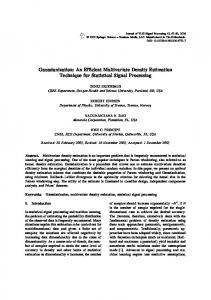
Figure 1: 2D classification problem created by a circle and the plane dividing two classes. Contours 0.2 0.4 0.6 0.8 of 5 Gaussians, 3 rectangles and a rectangle combined with Gaussians are shown. be tested first on artificial data. An interesting problem is defined by creating 2-class distribution of samples, with the first class separated from the second by a hyperplane with a spherical Gaussian placed at the border. In 2 dimensions this is a line with a circle. Training was done on 1400 randomly generated points, 600 on each side of the dividing hyperplane and 200 in the half-sphere. FSM network was set at 98% accuracy and training repeated 5 times. Networks created had 5.8±1.3 Gaussian nodes, 2.6±0.5 non-symmetric Gaussian nodes and 4.2±0.8 rectangular nodes. A network with mixed nodes found a solution with one rectangular node, extending through the whole data range, and one Gaussian node, substantially reducing the complexity of the final model (Fig. 1). The number of Gaussian or rectangular nodes in 3 to 5-dimensional cases grows quickly while the problem is still solvable by a single rectangular function providing a hyperplane, plus one Gaussian function. The FSM training algorithm is usually able to find the simplest solution but relatively large variance of results is obtained, indicating that the problem of finding an optimal solution is rather difficult. Tests on real data shows the ability of the FSM algorithm to find a small number of appropriate functions. For example, the Wisconsin cancer dataset [8] contains 699 instances, with 458 benign (65.5%) and 241 (34.5%) malignant cases. Each instance is described by the case number, 9 attributes with integer value in the range 1-10 (for example, feature f 2 is “clump thickness" and f 8 is “bland chromatin") and a binary class label. Performing 10-fold stratified crossvalidation with the target accuracy at the 96% level only 2 nodes using rectangular functions are created, giving a very simple description of the data in terms of logical rules. The actual accuracy achieved in 3 trials was 95.6, 95.4 and 95.4%, which compares favorably with slightly more accurate result of 96.5% that is obtained with 12 Gaussian functions, and with results of Shang and Breiman [9] who used CART decision tree achieving 93.5%, improved with boosting to 96.2%. Tests on several other datasets gave a reduction of the number of nodes created by the FSM network.
ESANN'2001 proceedings - European Symposium on Artificial Neural Networks Bruges (Belgium), 25-27 April 2001, D-Facto public., ISBN 2-930307-01-3, pp. 107-112
4
Conclusions
Networks using different transfer function open new possibilities for solving difficult classification problems and discovering simple representation of data, but also present new theoretical challenges. Finding the model with optimal complexity may be quite difficult although there are several algorithms based on information theory that may be helpful (cf. [10]. Numerical experiments performed so far indicate that the constructive algorithm used by FSM gives answers with a large variance, finding solutions of similar accuracy using different combination of functions. For real datasets it is quite probable that many such solutions exist. So far the FSM network has been tested with a few types of transfer functions in one network. One possibility that is worth exploring is to use families of transfer functions (Eq. 2, 3) that are parameterized to provide flexible decision borders. A single node is than able to provide a hyperplane or an ellipsoidal decision border. Results obtained with such networks should be reported soon.
References [1] C. Bishop, Neural networks for pattern recognition. Clarendon Press, Oxford, 1995. [2] W. Duch, G.H.F. Diercksen, Feature Space Mapping as a universal adaptive system, Computer Physics Communications 87, 341–371 (1995) [3] W. Duch, From cognitive models to neurofuzzy systems – the mind space approach. Systems Analysis-Modelling-Simulation 24, 53–65 (1996) [4] W. Duch, R. Adamczak, N. Jankowski, New developments in the Feature Space Mapping model. 3rd Conf. on Neural Networks, Kule, Poland, pp. 65-70 (1997) [5] W. Duch, R. Adamczak, N. Jankowski, Initialization of adaptive parameters in density networks. 3-rd Conf. on Neural Networks, Kule, Poland, pp. 99-104 (1997) [6] W. Duch and N. Jankowski, New neural transfer functions. Neural Computing Surveys 2, 639-658 (1999) [7] W. Duch and N. Jankowski, Taxonomy of neural transfer functions, Int. Joint Conference on Neural Networks, Vol. 3, pp. 477-484 (2000) [8] K. P. Bennett, O. L. Mangasarian, Robust linear programming discrimination of two linearly inseparable sets. Optimization Methods and Software 1, 23-34 (1992) [9] N. Shang, L. Breiman, Distribution based trees are more accurate. Int. Conf. on Neural Information Processing, Hong Kong, Vol. 1, pp. 133-138 (1996) [10] B. Ripley, Pattern Recognition and Neural Networks. Cambridge University Press (1996)