The second method concerns the incorporation of mixed state- ... attractive in aerospace industries. However ... The constraints are incorporated in the system.
JOURNAL OF GUIDANCE, CONTROL, AND DYNAMICS Vol. 31, No. 5, September–October 2008
Constructive Methods for Initialization and Handling Mixed State-Input Constraints in Optimal Control Knut Graichen∗ Vienna University of Technology, 1040 Vienna, Austria and Nicolas Petit† Ecole Nationale Supérieure des Mines de Paris, 75272 Paris, France DOI: 10.2514/1.33870 New methods are presented to address two issues in indirect optimal control: the calculation of a starting point for the numerical solution and the consideration of mixed state-input constraints. In the first method, an auxiliary optimal control problem is constructed from a given initial trajectory of the system. Its adjoint variables are simply zero. This auxiliary problem is then used within a homotopy approach to eventually reach the original optimal control problem and the desired optimal solution. The second method concerns the incorporation of mixed stateinput constraints into the dynamics of the considered optimal control problem. It uses saturation functions which strictly satisfy the constraints. In this way, the original constrained optimal control problem is transformed into an unconstrained one with an additional regularization term. The two approaches are derived within a general framework. For sake of illustration, they are applied to the space shuttle reentry problem, which represents a challenging benchmark due to its high numerical sensitivity and the presence of input and heating constraints. The reentry problem is solved with a collocation method and demonstrates the applicability and accuracy of the proposed constructive methods.
overcome this problem by combining indirect optimal control either with direct approaches [8–10] or with global methods, such as genetic algorithms [11]. However, all these approaches still require the direct method to obtain near-optimal initial guesses for the indirect solution or involve global optimization techniques to extend the region of convergence. 2) The analytical treatment of constraints within the indirect method is often nontrivial and leads to interior boundary conditions or case-dependent definitions of the control functions. In general, the overall structure of the boundary value problem (BVP) depends on the sequence between singular/nonsingular and unconstrained/ constrained arcs and requires a priori knowledge of the optimal solution. Motivated by the preceding problems, the scope of this paper is to present two new methods for initial guess calculation and for handling mixed state-input constraints in indirect optimal control: 1) The initial guess problem is addressed by presenting a new homotopy approach, which is based on an auxiliary optimal control problem (OCP) for which the adjoint states are simply zero. A continuation method is then employed to convert the auxiliary OCP to the original one. The auxiliary OCP can be derived for any given initial (not necessarily near-optimal) trajectory of the system, for example, obtained by forward integration. Hence, the homotopy approach can be seen as “self-contained,” because it does not require techniques from direct or global optimization. 2) A saturation function approach is presented to systematically account for mixed state-input constraints by adapting ideas originally developed in [12]. The constraints are incorporated in the system dynamics, which results in a new unconstrained OCP with an additional regularization term. Interestingly, the approach can be related to classical interior penalty function methods, whereby the idea of saturation functions circumvents certain numerical problems resulting in an enhanced numerical robustness. The two methods are presented in a general framework and are applied to the space shuttle reentry problem subject to input and heating constraints. The reentry problem is a frequently used benchmark in optimal control due to several challenging features, such as highly nonlinear dynamics and a high numerical sensitivity, see, for example, [4,13–18] for a collection of reentry problems and
I. Introduction
T
HE numerical solution of optimal control problems can be divided into different classes with their own advantages and characteristics. In the direct approach, the model equations of the considered system are discretized and the control trajectories are parametrized to obtain a finite-dimensional parameter optimization problem, see, for example, [1–4]. The well-known advantage of the direct approach is the good numerical robustness with respect to the initial guess, as well as the convenient handling of constraints. A different class of methods that gathered increasing interest in the recent past is global optimization, which explores the solution space of the optimization problem with the intention of finding all optimal solutions or solutions in unexpected regions. Typical solution techniques of global methods are genetic or evolutionary algorithms, which have, for example, been applied to find orbital or transfer trajectories [5,6]. Probably the most classical way to solve optimal control problems is the indirect approach, which is based on the calculus of variations and requires the solution of a two-point boundary value problem stemming from the first-order optimality conditions, see, for example, [7]. Indirect methods are known to show a fast numerical convergence in the neighborhood of the optimal solution and to deliver highly accurate solutions, which makes them particularly attractive in aerospace industries. However, two main drawbacks are opposed to the advantages of the indirect method: 1) A good initial guess of the trajectories (especially of the adjoint states) is required. This problem is of particular importance for highly sensitive problems. Several approaches have been proposed to Received 4 August 2007; revision received 1 March 2008; accepted for publication 18 March 2008. Copyright © 2008 by the American Institute of Aeronautics and Astronautics, Inc. All rights reserved. Copies of this paper may be made for personal or internal use, on condition that the copier pay the $10.00 per-copy fee to the Copyright Clearance Center, Inc., 222 Rosewood Drive, Danvers, MA 01923; include the code 0731-5090/08 $10.00 in correspondence with the CCC. ∗ Senior Researcher, Complex Dynamical Systems Group, Automation and Control Institute. † Assistant Professor, Centre Automatique et Systèmes. Member AIAA. 1334
1335
GRAICHEN AND PETIT
their numerical solution. The simulations for the reentry problem are conducted under MATLAB with a modified version of a collocationbased BVP solver. The numerical results reveal the good performance of the two presented methods and show the high accuracy of the indirect approach in optimal control. The paper is outlined as follows: The homotopy approach for the initial guess calculation is presented in Sec. II for a general class of unconstrained OCPs and is applied to the unconstrained reentry problem in Sec. III. Section IV derives the saturation function approach for general OCPs with mixed state-input constraints and discusses the numerical advantages with respect to classical penalty function methods. In Sec. V, the saturation function approach is applied to the reentry problem with input and heating constraints. The collocation code, which is used for the solution of the reentry problem is described in the Appendix.
II.
Homotopy Approach to Initial Guess Calculation
This section presents a new homotopy method to address the initial guess problem in indirect optimal control. An auxiliary OCP is derived with respect to a given initial trajectory of the system (e.g., obtained by integration) for which the adjoint states are simply zero. A continuation scheme is then used to convert the auxiliary OCP to the original one. For the sake of simplicity, the homotopy method is described for unconstrained OCPs. However, the method can equally be applied to the constrained case in Sec. IV, because the saturation function approach (presented in Sec. IV) results again in an unconstrained OCP. A.
Problem Statement
We consider the following OCP: min J�u� :� ’�x�T�; T� �
Z
T
L�x; u; t� dt
(1)
0
subject to x_ � f�x; u�;
x�0� � x0
(2)
The main obstruction in solving the BVP in Eqs. (2–7) is the initial guess of the adjoint trajectories ��t�, t 2 �0; T� and the guess of the free end time T. If ��t� and T are not sufficiently close to the optimal solution � �t� and T , the numerical solution of the BVP may not converge. As mentioned in the Introduction, several approaches exist in the literature to address this problem, see, for example, [8–10]. However, they typically require a near-optimal trajectory (usually by involving direct optimization methods) to calculate an initial trajectory for the adjoint state, which is sufficiently close to the optimal one. The focus of the next section is to construct an auxiliary OCP for a given (not necessarily near-optimal) trajectory of the system (2) for which the optimal solution of the adjoint state can easily be derived. This auxiliary OCP is then used in a homotopy approach to recover the original OCP in Eqs. (1–3). B.
Construction of Auxiliary Optimal Control Problem
In the first step, assume that an initial trajectory �x0 �t�; u0 �t��, t 2 �0; T 0 � with a certain final time T 0 is given, which satisfies the system equations and initial conditions in Eq. (2): x_ 0 � f�x0 ; u0 �;
x0 �0� � x0
In general, the final conditions of Eq. (3) for the end time T � T 0 will not evaluate to zero but to a certain residual � �x0 �T 0 �; T 0 � � �0T One possibility to derive the trajectory �x0 �t�; u0 �t�� is, for instance, a numerical integration of the system over the time interval t 2 �0; T 0 �. On the one hand, T 0 should be reasonably chosen within the range of the expected optimal final time T of the original OCP in Eqs. (1) and (2) and, on the other hand, with the objective to keep the residual �0T small. Consider now the auxiliary OCP ZT L0 �u; t� dt (8) min J0 �u� :� ’0 �T� � 0
0 � ��x�T�; T�
(3)
The nonlinear system (2) is described by f: Rn � Rm ! Rn with the state x 2 Rn and input u 2 Rm . The final conditions �: Rn � R� ! Rq in Eq. (3) are of dimension q � n. The cost functions ’: Rn ! R and L: Rn � R � �0; T� ! R, as well as f and �, are assumed to be sufficiently smooth. The end time T is unspecified for the sake of generality. However, the presented approach can also be applied to problems with fixed final time T. In the indirect approach to optimal control, the OCP in Eqs. (1–3) is treated with the calculus of variations. With the Hamiltonian H�x; �; u; t� � L�x; u; t� � �> f�x; u�
subject to x_ � f�x; u�;
0 � ��x�T�; T 0 � �0T
@H @L @f � �> �_ > � @x @x @x � � @’ � @� �� � > �T� � �� ��> @x T @x �T � � � � @’ � @� �� H�x; �; u; t��� � �� �> @t T @t �T T
(9) (10)
where the cost of Eq. (8) is defined by the functions 1 ’0 �T� � �T T 0 �2 ; 2
1 L0 �u; t� � ju�t� u0 �tT 0 =T�j2 (11) 2
with the Euclidean norm
the first-order optimality conditions for the OCP in Eqs. (1–3) follow to [7] @f @H @L � � �> �0 @u @u @u
x�0� � x0
(4) (5)
(6)
ju u0 j2 �
�ui u0i �2
i�1
Obviously, the optimal solution to the auxiliary OCP in Eqs. (8–10) is the previous trajectory �x0 �t�; u0 �t�� with the end time T � T 0 and the optimal cost J0 �u0 � � 0. Note that T 0 is used in the final conditions of Eq. (10) instead of the free end time T. This is of importance to obtain the optimal free end time T � T 0 , see Eq. (17). The time normalization �tT 0 =T� in Eq. (11) accounts for the fact that u0 �t� is only defined on �0; T 0 �. The derivation of the corresponding adjoint state ��t� � �0 �t� requires a closer look at the optimality conditions. The Hamiltonian
(7)
with the adjoint states � 2 Rn and the multipliers � 2 Rq . The unspecified end time T leads to the additional transversality condition (7). The optimal solution has to satisfy Eqs. (2–7) and is denoted by �x �t�; � �t�; u �t�; � ; T �, t 2 �0; T �.
m X
H0 �x; �; u; t� � L0 �u; t� � �> f�x; u�
(12)
yields @f @f @H 0 @L0 � �u u0 �tT 0 =T��> Im � �> � 0 (13) � � �> @u @u @u @u
1336
GRAICHEN AND PETIT
whereby @L0 =@u simplifies due to Eq. (11). The symbol Im denotes the (m � m) unit matrix. The adjoint system is defined accordingly by @H 0 @f � �> �_ > � @x @x � � � 0 � � @’0 �� > > @�� �T � � > @� � �� � �T� � � �� @x � @x @x �T T T
(14)
(15)
� �t� � 0;
� �0
0
0
t � �0; T �;
(16)
satisfies the optimality conditions (13–15). In addition, the transversality condition � � � 0 � � d’0 �� 0 > @�� �T � � 0 � � (17) H �x; �; u; t�� � � �T T @t dt �T T T must hold, due to the free end time T. As mentioned before, the function ��x�T�; T 0 � of the final conditions in Eq. (10) does not directly depend on T but on T 0 , which simplifies the right-hand side of Eq. (17) to T 0 T. For u�t� � u0 �t� and the trivial optimal adjoint state ��t� � �0 �t� � 0, the Hamiltonian (12) evaluates to zero and the transversality condition (17) yields T � T 0 as the optimal end time. Note that the derivation of the auxiliary OCP also holds if the final time T of the original OCP in Eqs. (1–3) is fixed. In this case, T 0 of the initial trajectory �u0 �t�; x0 �t��, t 2 �0; T 0 � must be chosen to T 0 � T and the transversality condition (17) is omitted. C.
Continuation Toward Original Optimal Control Problem
The auxiliary OCP in Eqs. (8–10) can be used as a starting point for a continuation scheme to eventually reach the original OCP in Eqs. (1–3). Thereby, the trajectory �x0 �t�; u0 �t��, t 2 �0; T 0 � with the trivial adjoint states �0 �t� � 0 and � � 0 forms the initial guess for the start of the continuation scheme. This leads to the following OCP: ZT L� �x; u; t� dt (18) min J� �u� :� ’� �x�T�; T� � 0
subject to x_ � f�x; u�;
x�0� � x0
h i 0 � �2 ��x�T�; T� � �1 �2 � ��x�T�; T 0 � �0T
(19) (20)
where the cost functions ’� �x�T�; T� � �1 ’�x�T�; T� � �1 �1 �’0 �T� L� �x; u; t� � �1 L�x; u; t� � �1 �1 �L0 �u; t�
(21)
are stated in dependence of a first continuation parameter �1 2 �0; 1� which converts the auxiliary cost in Eq. (8) for �1 � 0 to the original one in Eq. (1) for �1 � 1. The final conditions (20) couple Eqs. (3) and (10) via a second continuation parameter �2 2 �0; 1�. Hence, both parameters ��1 ; �2 � can be used to separately affect the cost in Eq. (18) and the final conditions (20). Starting at � � �0; 0� corresponds to the auxiliary OCP in Eqs. (8–10), whereas � � �1; 1� yields the original one in Eqs. (1–3). The optimality conditions are derived with the Hamiltonian H � �x; �; u; t� � L� �x; u; t� � �> f�x; u� and read @f @H � @L� �0 � � �> @u @u @u
�
� > �T� �
� � � � �� � @’� �� @’ �� > @� � > @� � �� �� �� 1 � � � @x T @x �T @x T @x T
� � � � @’� �� @�� �� > � H �x; �; u; t�� � � @t �T @t �T T � � @’ � @� �� � �1 �� �1 �1 ��T T 0 � �2 �> @t T @t �T
(23)
(24)
�
With x�t� � x0 �t� and u�t� � u0 �t� as the optimal solution to the OCP in Eqs. (8–10), it directly follows that the trivial solution 0
�
@H @L @f � �> �_ > � @x @x @x
(22)
(25)
The simplification of Eqs. (24) and (25) is due to the particular structure and dependencies of Eqs. (20) and (21). The Eqs. (19–25) define a two-point BVP for the states x�t�, ��t�, the multipliers �, the optimal control u�t�, and the end time T in dependence of the continuation parameters ��1 ; �2 �. The simplest way to solve the homotopy problem is to manually increase ��1 ; �2 � from (0, 0) to (1, 1) in N steps with N being sufficiently large. The first run ��11 ; �12 � of the homotopy is initialized with the auxiliary trajectory �x0 �t�; u0 �t�; �0 �t�; �0 ; T 0 � and �0 �t� � �0 � 0, whereas the subsequent steps ��i1 ; �i2 �, i � 2; . . . ; N use the solution of the previous run as initialization. Finally, the optimal solution �x �t�; u �t�; � �t�; � ; T � of the original OCP in Eqs. (1) and (2) is obtained for ��N1 ; �N2 � � �1; 1�. Because ��1 ; �2 � separately affects the cost in Eq. (18) and the boundary conditions (20), some freedom exists concerning how �1 and �2 are increased. In general, the number of steps N depends on the sensitivity of the problem and the length of the homotopy path. If the initial trajectory �x0 �t�; u0 �t�� is close to the optimal solution, N can usually be chosen smaller compared with the case in which the initial and optimal trajectories are far away from each other. A more sophisticated method than manually chosen N and the sequence for ��1 ; �2 � is differential homotopy, which dynamically follows the homotopy path by means of predictor–corrector schemes. A further method is simplicial homotopy, which subdivides the search space into cells by piecewise linear approximations. The advantage of the simplicial method is that it puts low requirements on the homotopy problem and involves no further derivatives as in the case of differential homotopy. On the other hand, the differential method generally converges faster due to the prediction behavior. More details on this topic can, for example, be found in [19,20]. Although these systematic methods may find solutions where the manual way of increasing ��1 ; �2 � fails, they require substantially more implementational effort. Moreover, these methods consider a single homotopy parameter compared to ��1 ; �2 � in OCP (18–21). This problem can be taken into account, for instance, by using �1 and �2 in a cascade of two single homotopies or by reducing them to a single parameter �1 � �2 . However, the separate consideration of both parameters �1 and �2 provides an additional degree of freedom, which can be used to find a suitable homotopy path.‡
III.
Example 1: Unconstrained Reentry Problem
An ideal example for the homotopy approach is the space shuttle reentry problem, due to its high numerical sensitivity and the relatively large reentry time interval �0; T�. Several different versions and problem formulations of the reentry OCP exist in the literature, see, for example, [4,8,17]. The reentry problem used in this paper is due to Betts [4]. The model equations and the optimal control objective are recapitulated before the homotopy approach is used to ‡ A special case occurs if the initial trajectory �x0 �t�; u0 �t��, t 2 �0; T 0 � directly satisfies Eq. (3), that is, ��x0 �T 0 �; T 0 � � 0, such that the boundary conditions (20) reduce to the original ones in Eq. (3) and �2 is not required. This is, for example, the case for flat systems, where �x0 �t�; u0 �t�� can be constructed in terms of the flat output and its time derivatives [21]. Alternatively, the approach in [22] can be adapted to determine �x0 �t�; u0 �t��, which satisfies the boundary conditions in Eqs. (2) and (3). Then, only �1 occurs and the differential or simplicial homotopy can more easily be applied.
1337
GRAICHEN AND PETIT
solve the reentry problem. The numerical results are obtained with a collocation solver under MATLAB (see Appendix). A.
B.
Adaption to Homotopy Formulation
The reentry model of Eqs. (26–31) can be put in the general form of Eq. (2) with the state and control vectors
Model Description
x � �h; v; �; �; �> ;
The equations of motion of the space shuttle, as stated in [4], are h_ � v sin � v_ �
�_ �
(26)
D�h; v; �� g�h� sin � m
(27)
� � L�h; v; �� v g�h� cos � � cos � mv Re � h v �_ �
v cos � cos Re � h
(29)
_ � L�h; v; �� sin � � v cos � sin mv cos � Re � h �_ �
(28)
sin �
(31)
with altitude h, velocity v, flight-path angle �, latitude �, azimuth , and longitude � as the states of the system. The controls of the space shuttle are the angle of attack � and the bank angle �. The gravity g�h� and atmospheric density ��h� are modeled by g�h� � �=�Re � h�2 ;
��h� � �0 exp� h=hr �
The objective of the reentry problem is to maximize the cross range, which corresponds to the final latitude x4 �T� � ��T�. Hence, the cost functions in Eq. (1) reduce to ’�x�T�� � x4 �T� and L�x; u; t� � 0, which yields the cost to be minimized J�u� :� x4 �T�
(39)
Note that T is not explicitly occurring in ��x�T�� and ’�x�T��. Moreover, the homotopy BVP formulation in Eqs. (19–25) simplifies for the reentry problem due to the explicit final conditions (24) and the simple final cost in Eq. (39). In particular, the final conditions (24) for the adjoint state ��t� and the transversality conditions (25) reduce to
i �T� � �i � free;
i � 1; 2; 3
4 �T� � �1 ;
5 �T� � 0 � � H� �x; �; u; t��� � �1 �1 ��T T 0 �
(32)
and are used to determine the lift and drag functions
(40)
(41)
T
1 L�h; v; �� � cL ���S� �h�v2 ; cL ��� � a0 � a1 �^ 2 �^ � 180�= 1 D�h; v; �� � cD ���S� �h�v2 ; 2
(37)
The longitude � and the ordinary differential equation (ODE) (31) are omitted because they are decoupled and do not affect the remaining ODEs (26–30). The initial conditions in Eq. (2) follow from Eq. (35). The final conditions (36) can be stated in terms of Eq. (3): 0 1 x1 �T� 80; 000 ft (38) � �x�T�� � @ x2 �T� 2500 ft=s A � 0 x3 �T� � 5 deg
(30)
v cos � sin = cos � Re � h
u � ��; ��>
(33)
cD ��� � b0 � b1 �^ � b2 �^ 2
The explicit calculation of the Lagrange multipliers �1 , �2 , �3 is not necessary, because they do not affect the transversality condition (41). Instead, the boundary conditions i �T�, i � 1, 2, 3 are treated as being free and are not considered (together with the multipliers �1 , �2 , �3 ) in the BVP formulation, see, for example, [7].
(34) C.
which appear in the system model of Eqs. (26–31). The corresponding parameters are listed in Table 1. The shuttle reentry is defined to start at the initial conditions h�0� � 260; 000 ft; v�0� � 25; 600 ft=s;
��0� � 0 deg;
��0� � 0 deg
��0� � 1 deg;
�0� � 90 deg (35)
The final point of the reentry trajectory occurs at the unknown end time T at the so-called terminal area energy management [4], which is defined by the conditions h�T� � 80; 000 ft;
v�T� � 2500 ft=s;
��T� � 5 deg (36)
The objective of the reentry problem is to maximize the cross range, which is equivalent to maximizing the latitude ��T�.
Numerical Results
The reentry problem is solved with the collocation method described in the Appendix. The optimality conditions (22–25) and the Jacobians are calculated with the computer algebra program MATHEMATICA and are provided as C-mex functions to MATLAB. The simulations are preformed on a PC equipped with an Intel CPU of the type Pentium Core Duo 1.6 GHz and 2 GB memory. To start the homotopy solution of the reentry problem outlined in Sec. II, an initial trajectory �x0 �t�; u0 �t�� is calculated by integrating the system Eqs. (19) over the time interval t 2 �0; T 0 � with the guessed end time T 0 � 1000 s and the chosen constant input u � ��; ��> � �30; 30�> deg. The trajectory �x0 �t�; u0 �t�� with the trivial adjoint state ��t� � �0 �t� � 0 is then used as an initial guess for the homotopy approach. As mentioned before, some freedom exists concerning the number of steps N and how the two homotopy parameters � � ��1 ; �2 � are increased to �N � �1; 1�. The best results for the reentry problem are obtained by first increasing �1 to smoothly convert the cost
Table 1 Parameters of the shuttle model Eqs. (26–34) taken from [4,13] Symbol
Value
Symbol
Value
Symbol
Value
� hr a0 b1 c1
0:1407654 � 1017 ft=s2 23,800 ft 0:20704 0:61592 � 10 2 0:19213774 � 10 1
�0 S a1 b2 c2
0:002378 lb=ft3 2690 ft2 0.029244 0:621408 � 10 3 0:21286289 � 10 3
Re m b0 c0 c3
20,902,900 ft 6309.44 lb 0.07854 1.06723181 0:10117249 � 10 5
GRAICHEN AND PETIT
0.3
velocity v [105 ft/s]
6
altitude h [10 ft]
1338
0.25 0.2 0.15 0.1 0
500
1000 time [s]
1500
0.25
st art: step 3: step 7: step 10: step 13: step 17: step 20:
0.2 0.15 0.1 0.05
2000
0
500
1000 time [s]
1500
κ0 =( κ3 =( κ7 =( κ 10 = ( κ 13 = ( κ 17 = ( κ 20 = (
0, 0) 0.3, 0) 0.7, 0) 1, 0) 1, 0.3) 1, 0.7) 1, 1)
2000
10 0 500
1000 time [s]
1500
30
zoom on α for κ 20 = ( 1, 1)
25 20 15
−2 −4 −6
2000
bank angle β [deg]
angle of attack α [deg]
0
0
0
500
1000 time [s]
1500
80 60 40 20 0
2000
0
heating q [BTU/ft2/s]
20
azimuth ψ [deg]
flight path γ [deg]
latitude θ [deg]
2 30
−20 −40 −60
500
1000 time [s]
1500
2000
Fig. 1
0
500
1000 time [s]
1500
500
1000 time [s]
1500
2000
0
500
1000 time [s]
1500
2000
150 100 50
−80 0
0
2000
0
Homotopy trajectories for the unconstrained reentry problem.
function (18) to the desired one in Eq. (39). This is done in 10 steps from �11 � 0:1 to �10 1 � 1, while keeping �2 � 0. Afterward, �2 is 20 increased similarly from �11 2 � 0:1 to �2 � 1 in 10 steps to force the boundary conditions (20) to the original values in Eq. (38). Figure 1 shows the reentry trajectories for several steps of the homotopy method. Clearly visible is the homotopy path from the initial trajectory for �0 � �0; 0� to the optimal solution for �20 � �1; 1� in the 20th step. This is particularly interesting because the initial trajectory �x0 �t�; u0 �t�� and the initial time T 0 � 1000 s are clearly far away from the optimal solution. An interesting phenomenon in the final trajectories are the oscillations, which occur due to the bumping of the space shuttle on the atmosphere during the reentry maneuver. These oscillations lead to a complex shape of the trajectories and illustrate the high sensitivity of the reentry problem. The trajectories in Fig. 1 also show that increasing �1 before �2 seems to lead to the most natural homotopy path, and indicates that the original cost [maximization of ��T�] is a more natural criterion in combination with the final conditions than the artificial cost of the auxiliary OCP. Compared with this homotopy path, other increasing sequences for ��1 ; �2 � led to significant gradients and oscillations in the controls u � ��; ��> during the single steps. Table 2 summarizes some details of the successive numerical solutions by means of the collocation code (see Appendix). The homotopy approach is started with the initial trajectory �x0 �t�; u0 �t��,
t 2 �0; T 0 �. The mesh refinement is turned off during the homotopy solution and the single trajectories are computed on the fixed mesh with 200 equidistant points. The reason for using a fixed mesh is that the mesh refinement leads to an increase of mesh points during the homotopy solution, where the shape of the trajectories strongly changes.§ A final run with activated mesh refinement leads to the optimal reentry trajectories (see Fig. 1) with 305 mesh points, the final time T � 2008:59 s and the maximum cross range ��T� � 34:1412 deg. The overall required CPU time for the numerical solution on the aforementioned PC is 46.2 s. The final trajectories in Fig. 1 are practically identical with the reference results [4], and the values of T and ��T� coincide with the reference values up to the last digits given in [4]. Moreover, the collocation solver converged during the single steps of the homotopy approach within 2–4 iterations. These observations agree with the common statement that the indirect method in optimal control shows a high accuracy and a good convergence behavior. In practice, the trajectories would have to be implemented in a closed loop to achieve stability and robustness with respect to perturbations. This can be done, for example, using the theory of neighboring extremals [23]. An alternative is the well-known 2 degrees-of-freedom control concept [24], where the optimal trajectory u �t� is used as a feedforward control together with a feedback part, which can be designed by linear methods.
Table 2 Statistics for the solution of the unconstrained reentry problem � � ��1 ; �2 �
Mesh points
T
��T�
CPU time
1–10 �10 � �1; 0� 11–20 �20 � �1; 1� Mesh refinement
200 (fixed) 200 (fixed) 305 (auto)
912.44 s 1967.01 s 2008.59 s
5.0148 deg 34.1421 deg 34.1412 deg
16.1 s 25.6 s 4.5 s
Steps
§ With activated mesh refinement, the steps for increasing ��1 ; �2 � have to be chosen smaller to keep the number of grid points within reasonable limits.
1339
GRAICHEN AND PETIT
IV. Incorporation of Mixed State–Input Constraints In this section, the unconstrained OCP in Eqs. (1–3) is extended by mixed state-input constraints of the form di �x; ui � 2 �di ; di� �;
i � 1; . . . ; m
(42)
which are assumed to be well defined with respect to the single inputs ui of the control vector u � �u1 ; . . . ; um �> , that is, @di =@ui ≠ 0. Although it is possible to analytically consider the constraints in indirect optimal control, it generally requires a priori knowledge of the switching structure of the optimal solution and leads to interior boundary conditions, which complicate the BVP in Eqs. (2–7) of the optimality conditions. The saturation function approach presented in this section circumvents this problem and incorporates the constraints within the system dynamics by following the ideas in [12], originally developed in the context of feedforward control design. This procedure results in a new unconstrained OCP with an additional regularization term. Interestingly, the approach can be related to classical penalty function methods, while avoiding their numerical difficulties. A.
ui 2 �u i �x�; u� i �x��;
i � 1; . . . ; m
(43)
with the state-dependent lower and upper limits u i �x� and u� i �x�. In � the case of pure input constraints, the limits u� i �x� � ui are independent of x. The reformulated constraints (43) are now represented by saturation functions ui �
~ i �; i �x; u
i � 1; . . . ; m
(44)
with the new unconstrained inputs u~ � �u~ 1 ; . . . ; u~ m �> . It is assumed that the saturation functions i �x; u~ i � reach their limits u� i �x� only asymptotically for u~ i ! �1, see Fig. 2. An appropriate choice for ~ i � is, for example, i �x; u ~i� i �x; u
�
u� i �x�
u� �x� u i �x� i ; 1 � exp�su~ i �
0
subject to ~ u�; ~ x_ � f�x;
x�0� � x0
(47)
0 � ��x�T�; T�
(48)
where the cost functional
~2� juj
m X
u~ 2i
i�1
and the parameter " > 0 is necessary to account for the influence of the saturation close to the constraints in Eq. (43). This point can be explained with the Hamiltonian ~ u� ~ �; u; ~ u; ~ ~ t� � L�x; ~ t� � "juj ~ 2 � �> f�x; H�x; ~ u~ � 0 with respect to the new and the optimality conditions @H=@ input u~ � �u~ 1 ; . . . ; u~ m �> : @L~ @f~ @H~ � � 2"u~ i � �> � 0; @u~ i @u~ i @u~ i
i � 1; . . . ; m
(49)
~ the partial derivatives Because of the input substitution u � �x; u�, in Eq. (49) evaluate to¶ � � @L �� @ i @f~ @f �� @ i @L~ � ; � @u~ i @ui ��44� @u~ i @u~ i @ui ��44� @u~ i These relations show that if one of the original inputs ui approaches the respective constraints (43), the corresponding i �x; u~ i � will also approach saturation with the gradient @ i =@u~ i tending to zero (cf. Fig. 2). Hence, the regularization terms 2"u~ i in Eq. (49) are used to still be able to compute the new input u~ � �u~ 1 ; . . . ; u~ m �> from Eq. (49) if one or several gradient terms are vanishing due to saturation. To complete the optimality conditions, the adjoint state � and the free end time T are given by @H~ @L~ @f~ � �> �_ > � @x @x @x � > �T� �
� � � @’ �� > @� � �� � @x T @x �T
� � � � @’ � @� �� ~ �; u; ~ t��� � �� �> H�x; @t T @t �T T with the partial derivatives � � @L~ � @L �� � @L �� @ ; @x ��44� @u ��44� @x @x
(50)
(51)
(52)
� � @f~ @f �� @f �� @ � � @x @x ��44� @u ��44� @x
and the vector of saturation functions � � 1 ; . . . ; m �> . The Eqs. (47–52) form a two-point BVP for the regularized OCP in Eqs. (46–48) with the parameter ". The desired optimal solution �x �t�; u �t��, t 2 �0; T � of the OCP (1–3) subject to the constraints (43) can be approached by using a continuation scheme to successively decrease the regularization parameter ".
ψi
B.
0
An interesting feature of the saturation function approach is that it has some similarity to classical interior penalty methods, see, for example, [25,26]. This relation can be used to give more insight into the regularization term and to emphasize some numerical advantages of the saturation function formulation.
u +i (x )
u˜i
u −i (x ) Fig. 2
~ u; ~ t� dt L�x;
~ t� and the new system function f~ � with L~ � L�x; �x; u�; ~ follow from Eqs. (1) and (2). f�x; �x; u�� The additional regularization term in Eq. (46) with
4 s� � ui �x� u i �x� (45)
where the parameter s normalizes the slope @ i =@u~ i � 1 at u~ i � 0. The inputs u of the original OCP in Eqs. (1–3) can be replaced by ~ where � � 1 ; . . . ; m �> denotes the vector over all u � �x; u�, saturation functions (45). This leads to the following unconstrained OCP ZT ~ u� ~ :� J� ~ �"� ~ 2 dt juj (46) min J~" �u�
T 0
Incorporation of Constraints with Saturation Functions
Because it is assumed that the functions di �x; ui � are well defined with respect to ui , that is, @di =@ui ≠ 0, the mixed state-input constraints (42) can be written as input constraints
Z
~ u� ~ :� ’�x�T�; T� � J�
Saturation function ui �
~ i �. i �x; u
Comparison with Interior Penalty Functions
¶ The compact notation � �j�44� signifies the substitution of the original input u � �u1 ; . . . ; um �> by the saturation functions (44).
1340
GRAICHEN AND PETIT 2
ε ψi− 1(x , u i )
are obtained under MATLAB with the collocation method described in the Appendix. A.
Input and Heating Constraints
In addition to the reentry model in Sec. III.A., the problem formulation in [4] includes constraints on the controls � and � � 2 � 90; 90� deg;
ε
ε
� 2 � 89; 1� deg
(56)
as well as an additional constraint on the aerodynamic heating on the shuttle wing leading edge q�h; v; �� � q� � 70 Btu=ft2 =s
u −i (x )
where the heating q�h; v; �� is defined as a function of the states h, v, and the control �:
u +i (x ) u i �1 2 i �x; ui ��
Fig. 3 Interior penalty term �
with parameter " > 0.
The new inputs u~ i in the regularization term of the cost in Eq. (46) can be expressed by the inverse relations of the saturation functions (44) 1 i �x; ui �;
u~ i �
i � 1; . . . ; m
(53)
which allows one to rewrite the regularized cost of Eq. (46) in terms of the original inputs u � �u1 ; . . . ; um �> : ZT L�x; u; t� � "j 1 �x; u�j2 dt (54) J" �u� :� ’�x�T�; T� �
q�h; v; �� � qa ���qr �h; v� �^ � 180�= qa ��� � c0 � c1 �^ � c2 �^ 2 � c3 �^ 3 ; p���������� 4 3:07 qr �h; v� � 17; 700 ��h��10 v�
qa ��� �
1 � �u� �x� u i �x��flog�ui u i �x�� 4 i log�u� i �x� ui �g
(55)
Obviously, the term j
1 2
j �
m � X
1 i
�2
i�1
shows a logarithmic barrier behavior, which penalizes the inputs ui if they approach the constraints (43), see Fig. 3. From this point of view, the saturation function approach has some similarity with classical interior penalty methods, see, for example, [25,26]. However, a well-known problem of interior penalty methods is that special care has to be taken that iterates during the numerical solution of the OCP do not violate the barriers u� i �x�. The saturation function approach circumvents this problem of interior penalty methods by incorporating the constraints (43) directly within the unconstrained OCP (46–48) with the new inputs u~ i . Hence, the saturation functions (45) force the inputs ui to strictly remain inside the constraints (43), which results in a truly unconstrained problem. This formulation has numerical advantages, because iterates during the numerical solution cannot violate the constraints. For instance, the regularization parameter " can usually be decreased in larger steps to converge more rapidly to the optimal solution. A further advantage is that the constraints (43) can be reduced from one OCP solution to the next, for example, to start from an unconstrained solution. This aspect is illustrated for the reentry problem in the next section.
q� qr �h; v�
(59)
to limit the heating to the maximum allowed value in Eq. (57). As shown in Fig. 4, the function qa ��� is monotonically decreasing with respect to �. Hence, in each time instant t, a lower limit � for � � can be calculated from Eq. (59) with respect to the instantaneous states h and v, that is, � � q� (60) � �h; v� � q 1 a qr �h; v� In this way, the heating constraint (57) can be accounted for by replacing the lower bound of � in Eq. (56) by the state-dependent limit � �h; v�. This leads to the (partially state-dependent) input constraints � 2 �� �h; v�; 90 deg�;
� 2 � 89; 1� deg
(61)
with the constant values taken from Eq. (56). In general, the function qa ��� is not analytically invertible, since qa ��� may be derived as an interpolation between measurement data, which leads, for instance, to a polynomial function as in Eq. (58). The analytic inversion (60) can be avoided by numerically solving the algebraic equation 1.1 1 function qa(α) [−]
1 1 > � � 1 with the vector 1 ; . . . ; m � . Using the explicit formula (45) for i �x; u~ i �, the inverse relations 1 i �x; ui � read
(58)
The parameters occurring in Eq. (58) are listed in Table 1. The heating constraint (57) represents a mixed state-input constraint of the form in Eq. (42), which can be rearranged such that qa ���, as a function of the angle of attack �, has to satisfy the inequality
0
1 i �x; ui �
(57)
0.9 0.8 0.7 0.6
V. Example 2: Constrained Reentry Problem In this section, the unconstrained reentry problem in Sec. III is extended by additional input and heating constraints, which are handled by means of the saturation functions. The unconstrained optimal solution obtained by the homotopy approach (see Fig. 1) is used as an initial guess for the constrained case. The numerical results
0.5 0
10
20 30 angle of attack α [deg]
40
50
Fig. 4 Heating function qa ��� in Eq. (58) plotted over the angle of attack �.
1341
velocity v [105 ft/s]
0.25
6
0.2 0.15 0.1 1000 1500 time [s]
q+ = 140 BT U/ ft 2 / s , ε = 10− 6
0.15
q+ = 120 BT U/ ft 2 / s , ε = 10− 6 q+ = 80 BT U/ ft 2 / s , ε = 10− 6
0.05
2000
q+ = 70 BT U/ ft 2 / s , ε = 10− 10 0
30 20 10 0
500
500
1000 1500 time [s]
2000
0 −1 −2 −3 −4
80 60 40 20
−5
2000
0
25
20
500
1000 1500 time [s]
2000
0
2
bank angle β [deg]
30
−20 −40 −60
500
1000 1500 time [s]
2000
0
Fig. 5
500
(62)
for � in each time instant. Numerical Results
Similar to the unconstrained case, the shuttle ODEs (26–30) can be written in the form of Eq. (47) with the state and control vectors of Eq. (37), the final conditions (38), and the final cost in Eq. (39). The constrained inputs u � ��; ��> in Eq. (61) are replaced by saturation functions according to Eq. (44), ~ 1 �h; v; ��;
��
500
1000 1500 time [s]
2000
0
500
1000 1500 time [s]
2000
100 50 0
2000
Optimal trajectories for the constrained reentry problem.
qa �� �qr �h; v� q� � 0
��
1000 1500 time [s]
0
150
−80 0
B.
1000 1500 time [s]
0 0
angle of attack α [deg]
q+ = 100 BT U/ ft 2 / s , ε = 10− 6
0.1
azimuth ψ [deg]
500
0.2
flight path γ [deg]
latitude θ [deg]
0
unconstrained solution
0.25
heating q [BTU/ft /s]
altitude h [10 ft]
GRAICHEN AND PETIT
~
2 ���
(63)
~ > . The two-point BVP ~ �� with the new unconstrained inputs u~ � ��; in Eqs. (47–52) is solved under MATLAB with the collocation code described in the Appendix.∗∗ The constrained trajectories for the reentry problem are obtained by starting from a sufficiently large value q� of the heating constraint q � q� and successively reducing q� until the desired constraint (57) is reached. This is done in five steps with the decreasing constraints q� 2 f140; 120; 100; 80; 70g Btu=ft2 =s
q� � 70 Btu=ft2 =s is reached, the penalty parameter " is gradually decreased to " � 10 10 to approach the optimal solution. Figure 5 shows the computed trajectories of the shuttle reentry for the decreasing constraints (64) as well as the final solution for the penalty parameter " � 10 10 . The reduction of the heating constraints (64) in only five steps shows the robustness of the saturation function approach with respect to the constraints. The heating profiles q�t� for the single steps from " � 10 6 to " � 10 10 are additionally depicted in Fig. 6. Clearly visible in Figs. 5 and 6 is the adherence of the heating constraint by the single trajectories and the different shapes of the reentry trajectories compared with the unconstrained one. The distance of q�t� to the constraint q� � 70 Btu=ft2 =s is negligible for " � 10 10 , although the saturation functions in Eq. (63) are only of asymptotic nature, which means that ~ does not exactly reach the lower constraint � � � � 1 �h; v; �� � �h; v� corresponding to the heating constraint (57). The statistics of the numerical solution of the constrained reentry problem are listed in Table 3. In the first part of the solution, when the
ε= ε= ε= ε= ε=
70
(64) 2
heating q [BTU/ft /s]
60
For the first run with q� � 140 Btu=ft2 =s, the unconstrained optimal solution (see Fig. 1) is used as an initial guess for the collocation ~ ~ method. The corresponding new input trajectories ��t� and ��t� directly follow from the inverse saturation functions (53), whereas the initial profile of the lower constraint � �t� is obtained by numerically solving Eq. (62) with the MATLAB function fsolve of the Optimization Toolbox. Because of the expected large final time of approximately T � 2000 s, the initial penalty parameter is chosen to " � 10 6 to ensure that the integrated penalty in Eq. (46) lies within the range of the final cost of the reentry problem. After
50 70.01
40 70
30 69.99
20 69.98
10
69.97
The implicit Eq. (62) for the lower constraint � � � �h; v� on � is treated as an additional algebraic equation in Eq. (A2), such that the vector of ~ � �> . ~ �; algebraic variables comprises z � ��;
300
600
900
1200
0 0
∗∗
10− 6 10− 7 10− 8 10− 9 10− 10
500
1000 time [s]
1500
2000
Fig. 6 Constrained heating trajectories q�t� for decreasing penalty parameters ".
1342
GRAICHEN AND PETIT
Table 3 Statistics for the solution of the constrained reentry problem Steps
Mesh points �
Option 1: decrease of q �" � 10 � 5 steps, see Eq. (64) 200 (fixed) Option 2: homotopy (" � 10 6 ) 10 steps: �10 � �1; 0� 200 (fixed) 200 (fixed) 10 steps: �20 � �1; 1� Subsequent decrease of " in 4 steps with mesh refinement 7 779 (auto) " � 10 807 (auto) " � 10 8 " � 10 9 809 (auto) 814 (auto) " � 10 10
heating constraint (64) is successively decreased (see “Option 1” in Table 3), the mesh refinement is turned off to avoid the increase of mesh points due to the strongly changing shape of the trajectories in the single steps. An alternative to lowering the heating constraint (64) is to use the homotopy approach in Sec. II, similar to the unconstrained reentry problem. The details and the respective simulation results are omitted here due to the lack of space. Nevertheless, the statistics are included in Table 3 (see “Option 2”) and are based on the same initial trajectory �x0 �t�; u0 �t�� and the same steps of the continuation parameters � � ��1 ; �2 � as in Sec. III.C. For both options 1 and 2, the resulting trajectories for the heating constraint q� � 70 Btu=ft2 =s and the penalty parameter " � 10 6 are practically identical and thus yield the same results in the subsequent reduction of ", see Table 3. Thereby, the mesh refinement is active and the last run with " � 10 10 yields the final trajectory in Fig. 6 with 814 mesh points. The optimal final time T � 2198:67 s and the maximum cross range ��T � � 30:6255 deg coincide with the reference results in [4] (up to the last digits given in [4]). This, in particular, shows the negligible influence of the remaining penalty term in Eq. (46) for " � 10 10 . Because of the increased number of mesh points, the overall CPU times for options 1 and 2 are significantly higher than for the unconstrained reentry problem (see Table 2) and amount to 340.8 and 359.4 s, respectively.
VI.
T
��T�
CPU time
6
2194.51 s
30.59 deg
54.8 s
941.34 s 2194.51 s
4.183 deg 30.59 deg
19.3 s 54.1 s
2197.68 s 2198.51 s 2198.65 s 2198.67 s
30.6208 deg 30.6249 deg 30.6254 deg 30.6255 deg
reentry problem. They appear to be well suited for aerospace trajectory optimization problems and are currently used, along with ideas from nonlinear geometric control, on various ascent and reentry problems.
Appendix: Solution of Optimal Control Problems with Collocation The two-point BVPs of the reentry problem arising from the optimality conditions are numerically solved with a collocation method. Compared with shooting or gradient algorithms, the collocation method has advantages in handling final conditions and the inherently unstable process of system and adjoint equations.†† Moreover, additional algebraic equations such as Eq. (22) or Eq. (49), which extend the two-point BVP to a system of differential– algebraic equations (DAE), can be readily taken into account with the collocation method due to the discretization over the whole time interval. The basis for the numerical solution of the reentry problems in this paper is the standard MATLAB BVP solver bvp4c, which solves nonlinear two-point BVPs by means of the collocation method [29]. To be applicable to optimal control problems, we extended the bvp4c-code to the general BVP formulation of (index 1) differential– algebraic equations
Conclusions
The motivation of the paper was twofold: in the first part, a homotopy approach was presented to address the initial guess problem in optimal control. The homotopy approach relies on an auxiliary optimal control problem, which can be constructed for any given (not necessarily near-optimal) trajectory of the system. For instance, the initial trajectory for the reentry problem was far away from the final optimal solution and was obtained by a simple time integration. In general, however, the homotopy path to the final optimal solution is naturally shorter if the initial trajectory is chosen closer to the optimal one. Further research concerns the automation of the homotopy steps by means of search algorithms or differential/ simplicial homotopy. The second part of the paper presented a saturation function approach to systematically incorporate mixed state-input constraints into a new unconstrained optimal control problem with an additional regularization term. An interesting relation exists to classical interior penalty function methods, whereby the saturation function formulation has advantages concerning the numerical solution. For instance, the constraints can be successively reduced to start from an unconstrained trajectory. This has been demonstrated for the reentry problem with input and heating constraints. Current research is spent on extending the saturation function approach to a more general class of state and input constraints. Both presented approaches are connected in the sense that the saturation function approach results again in an unconstrained optimal control problem, to which the homotopy method can be applied to initialize its numerical solution. The proposed methods seem to have potential in the field of optimal control, because they are easy to implement and proved efficient on the reportedly difficult
51.0 s 109.3 s 70.6 s 55.1 s
y_ � f�y; z; t; p�;
t 2 �t0 ; tf �
(A1)
0 � g�y; z; t; p�;
t 2 �t0 ; tf �
(A2)
0 � h�y�t0 �; y�tf �; z�t0 �; z�tf �; p�
(A3)
with dynamic and algebraic states y�t�, z�t�, t 2 �t0 ; tf �. Moreover, unknown parameters p can additionally be considered in the DAE formulation in Eqs. (A1–A3). The general collocation method and its implementation in bvp4c has been left unchanged, as it was designed to be applicable and numerically robust for a wide range of BVPs. The collocation method in bvp4c discretizes the time interval �t0 ; tf � with J � 1 points t0 < t1 < < tJ 1 < tJ � tf
(A4)
and approximates the ODEs (A1) by means of the Simpson formula with fourth-order accuracy [29]. The discretized system Eqs. (A1), together with the boundary conditions (A3) and the algebraic Eqs. (A2), evaluated at all time points (A4), results in a set of nonlinear algebraic equations ^ 0 � F�Y�
(A5)
� � ^> ^> ^> ^> ^> Y^ > � y^ > J ;z J ;p 0 ;z 0 ;y 1 ;z 1 ;...;y
(A6)
with the vector
†† More information on the numerical solution of OCPs can, for example, be found in the textbooks [7,27]. A detailed analysis of the collocation method is given in [28].
GRAICHEN AND PETIT
comprising the approximate solutions y^ i � y�ti �, z^ i � z�ti �, i � 0; 1; . . . ; J, and the unknown parameters p. The residual Eqs. (A5) are numerically solved by a Newton iteration scheme �k 1� � Y^ �k� � G�Y^
(A7)
which starts from an initial guess Y^ �0� provided by the user. Moreover, the Newton iterations (A7) require the evaluation of the Jacobians of the right-hand-side functions in Eqs. (A1–A3), with respect to their arguments. To apply the collocation method to the homotopy approach, the BVP in Eqs. (19–25) has to be adapted to the DAE form of Eqs. (A1– A3).‡‡ The original and adjoint equations in Eqs. (19) and (23) form the dynamics of Eq. (A1) for the overall dynamic state y> � �x> ; �> �. The input vector u forms the algebraic variables z � u with Eq. (22) corresponding to the algebraic Eq. (A2). The boundary conditions for x and � in Eqs. (19), (20), and (24), together with the transversality conditions (25) form Eq. (A3). The free end time T is taken into account by means of the time transformation t � " ;
T � ";
d 1 d � dt " d
(A8)
with the normalized time coordinate 2 �0; 1�. Hence, the scaling factor " is treated as free parameter p � " in the DAE system (A1– A3) and the new time coordinate replaces t 2 �t0 ; tf � with the normalized interval boundaries t0 � 0 and tf � 1. In general, the multipliers � can be added to the parameter vector p> � �"; �> �. For the reentry problem, � was omitted due to the explicit structure of the final conditions in Eq. (38), also see Eqs. (40) and (41).
References [1] Hargraves, C., and Paris, S., “Direct Trajectory Optimization Using Nonlinear Programming and Collocation,” Journal of Guidance, Control, and Dynamics, Vol. 10, No. 4, 1987, pp. 338–342. [2] Seywald, H., “Trajectory Optimization Based on Differential Inclusion,” Journal of Guidance, Control, and Dynamics, Vol. 17, No. 3, 1994, pp. 480–487. [3] Betts, J. T., “Survey of Numerical Methods for Trajectory Optimization,” Journal of Guidance, Control, and Dynamics, Vol. 21, No. 2, 1998, pp. 193–207. [4] Betts, J. T., Practical Methods for Optimal Control Using Nonlinear Programming, Society for Industrial and Applied Mathematics, Philadelphia, PA, 2001, Chap. 5. [5] Gurfil, P., and Kasdin, N. J., “Niching Genetic Algorithms-Based Characterization of Geocentric Orbits in the 3D Elliptic Restricted Three-Body Problem,” Computer Methods in Applied Mechanics and Engineering, Vol. 191, Nos. 49–50, 2002, pp. 5683–5706. doi:10.1016/S0045-7825(02)00481-4 [6] Vasile, M., Summerer, L., and De Pascale, P., “Design of Earth–Mars Transfer Trajectories Using Evolutionary-Branching Technique,” Acta Astronautica, Vol. 56, No. 8, 2005, pp. 705–720. doi:10.1016/j.actaastro.2004.12.002 [7] Bryson, A. E., and Ho, Y.-C., Applied Optimal Control, Ginn, Waltham, MA, 1969, Chaps. 2–3. [8] von Stryk, O., and Bulirsch, R., “Direct and Indirect Methods for Trajectory Optimization,” Annals of Operational Research, Vol. 37, Nos. 1–4, 1992, pp. 357–373. doi:10.1007/BF02071065 [9] Martell, C. A., and Lawton, J. A., “Adjoint Variable Solutions via an Auxiliary Optimization Problem,” Journal of Guidance, Control, and Dynamics, Vol. 18, No. 6, 1995, pp. 1267–1271. [10] Seywald, H., and Kumar, R. R., “Method for Automatic Costate Calculation,” Journal of Guidance, Control, and Dynamics, Vol. 19, No. 6, 1996, pp. 1252–1261. [11] Wuerl, A., Crain, T., and Braden, E., “Genetic Algorithms and Calculus of Variations–Based Trajectory Optimization Technique,” Journal of
‡‡ The BVP in Eqs. (47–52) of the saturation function approach in Sec. IV can be adapted to the DAE form of Eqs. (A1–A3) in the same way.
1343
Spacecraft and Rockets, Vol. 40, No. 6, 2003, pp. 882–888. [12] Graichen, K., “Feedforward Control Design for Finite–Time Transition Problems of Nonlinear Systems with Input and Output Constraints,” Ph.D. Thesis, Universität Stuttgart, Shaker Verlag, Aachen, Germany, 2006, Chaps. 3–5, http://elib.uni-stuttgart.de/opus/volltexte/2007/ 3004. [13] Neckel, T., Talbot, C., and Petit, N., “Collocation and Inversion for a Reentry Optimal Control Problem,” Proceedings of the 5th International Conference on Launcher Technology, Centre National d’Etudes Spatiales Paper No. S17.4, 2003. [14] Désidéri, J.-A., Peigin, S., and Timchenko, S., “Application of Genetic Algorithms to the Solution of the Space Vehicle Reentry Trajectory Optimization Problem,” French National Inst. for Research in Computer Science and Control (INRIA) Research Rept. No. 3843, Sophia Antipolis, France, 1999. [15] Gang, C., Zi-ming, W., Min, X., and Si-lu, C., “Genetic Algorithm Optimization of RLV Reentry Trajectories,” Proceedings AIAA/CIRA 13th International Space Plane and Hypersonic System and Technology Conference, AIAA Paper 2005–3269, 2005. [16] Pesch, H. J., “A Practical Guide to the Solution of Real–Life Optimal Control Problems,” Control and Cybernetics, Vol. 23, Nos. 1–2, 1994, pp. 7–60. [17] Kreim, H., Kugelmann, B., Pesch, H. J., and Breitner, M. H., “Minimizing the Maximum Heating of a Reentry Space Shuttle: An Optimal Control Problem with Multiple Control Constraints,” Optimal Control Applications and Methods, Vol. 17, No. 1, 1996, pp. 45–69. doi:10.1002/(SICI)1099-1514(199601/03)17:13.0.CO;2-X [18] Bonnard, B., Faubourg, L., Launay, G., and Trélat, E., “Optimal Control with State Constraints and the Space Shuttle Re–Entry Problem,” Journal of Dynamical and Control Systems, Vol. 9, No. 2, 2003, pp. 155–199. doi:10.1023/A:1023289721398 [19] Allgower, E., and Georg, K., Numerical Continuation Methods. An Introduction, Springer, Berlin, 1990, Chaps. 2, 12–14. [20] Haberkorn, T., Martinon, P., and Gergaud, J., “Low Thrust MinimumFuel Orbital Transfer: A Homotopic Approach,” Journal of Guidance, Control, and Dynamics, Vol. 27, No. 6, 2004, pp. 1046–1060. doi:10.2514/1.4022 [21] Fliess, M., Lévine, J., Martin, P., and Rouchon, P., “Flatness and Defect of Nonlinear Systems: Introductory Theory and Examples,” International Journal of Control, Vol. 61, No. 6, 1995, pp. 1327–1361. doi:10.1080/00207179508921959 [22] Graichen, K., Hagenmeyer, V., and Zeitz, M., “A New Approach to Inversion–Based Feedforward Control Design for Nonlinear Systems,” Automatica, Vol. 41, No. 12, 2005, pp. 2033–2041. doi:10.1016/j.automatica.2005.06.008 [23] Pesch, H. J., “Real-Time Computation of Feedback Controls for Constrained Optimal Control Problems, Part 1: Neighboring Extremals,” Optimal Control Applications and Methods, Vol. 10, No. 2, 1989, pp. 129–145. doi:10.1002/oca.4660100205 [24] Horowitz, I. M., Synthesis of Feedback Systems, Academic Press, New York, 1963, Chap. 6. [25] Lasdon, L. S., Waren, A. D., and Rice, R. K., “An Interior Penalty Method for Inequality Constrained Optimal Control Problems,” IEEE Transactions on Automatic Control, Vol. 12, No. 4, 1967, pp. 388–395. doi:10.1109/TAC.1967.1098628 [26] Bonnans, J. F., and Guilbaud, T., “Using Logarithmic Penalties in the Shooting Algorithm for Optimal Control Problems,” Optimal Control Applications and Methods, Vol. 24, No. 5, 2003, pp. 257–278. doi:10.1002/oca.730 [27] Pytlak, R., Numerical Methods for Optimal Control Problems with State Constraints, Springer, Berlin, 1999, Chaps. 3–6. [28] Ascher, U. M., Mattheij, R. M. M., and Russell, R. D., Numerical Solution of Boundary Value Problems of Ordinary Differential Equations, Prentice–Hall, Englewood Cliffs, NJ, 1988, Chap. 5. [29] Kierzenka, J., and Shampine, L. F., “A BVP Solver Based on Residual Control and the Matlab PSE,” ACM Transactions on Mathematical Software, Vol. 27, No. 3, 2001, pp. 299–316. doi:10.1145/502800.502801