Forward Selection Initialization Method for Constructive Neural Networks

Forward Selection Initialization Method for Constructive Neural Networks JANI LAHNAJÄRVI, MIKKO LEHTOKANGAS, AND JUKKA SAARINEN Digital and Computer Systems Laboratory Tampere University of Technology P.O.BOX 553, FIN-33101 Tampere FINLAND

Abstract: In this paper we present an initialization method of hidden unit weights for cascade-correlation type constructive neural networks. The forward selection initialization (FSI) method uses a large pool of randomly initialized hidden units and then selects the best one of them by some predetermined criterion which in our simulations was the objective function used in the hidden unit training. The best unit is then trained to the final solution by a desired training algorithm as normally and it is installed in the active network. In total we studied five different algorithms with FSI method that were compared both in classification and regression problems to the basic versions of the same algorithms. The investigated algorithms were Cascade-Correlation, Modified Cascade-Correlation, Cascade, Cascade Network, and Fixed Cascade Error. The simulation results show that the proposed initialization method is beneficial not only in rather simple but also in highly complicated problems when compared to the corresponding algorithms using only single randomly initialized candidate units in the hidden unit training. Key-Words: Constructive neural networks, initialization, cascade-correlation, forward selection, classification, regression.

1 Introduction The learning problem for neural networks can be viewed as a nonlinear optimization problem in which the goal is to find the set of network weights that minimizes a performance function. The performance function, which is usually a function of the network mapping errors, describes a surface in the weight space, often referred to as the error surface. Training methods can then be regarded as methods for searching this surface for a minimum. The complexity of the search is governed by the nature of the surface. Error surfaces in most neural networks have several wellknown characteristics that make them difficult to search. For example, they have many flat regions where learning is slow, and long narrow troughs that are flat in one direction and steep in surrounding directions. In addition, the error surface is usually characterized by a large number of poor local minima in the neighbourhood of an acceptable local or a global minimum.

In any nonlinear optimization problem, the initialization of the parameters has an important influence on the ability of the training algorithm to converge and the speed of that convergence. Since the network weights are normally initialized randomly, a large number of networks with different weight initializations may need to be trained before a weight initialization is found which converges to a good solution. An extensive search for the optimum values requires therefore much more overhead than performing a relatively small number of simulations using near-optimal values. In practise, however, it is not feasible to perform a global search for obtaining the optimal values of the initial network weights or other parameters. Furthermore, current mathematical techniques are insufficient for a complete theoretical study of the learning behaviour of the neural networks. Nevertheless, it is important to have a good approximation of the optimal initial values of the parameters to reduce the required training time. For those reasons, computationally more efficient

weight initialization methods are needed for the better training of neural networks. This research is focused on applying a forward selection initialization (FSI) [5] method for constructive neural network algorithms. Especially some cascade-correlation type algorithms have been studied. The idea of the cascade-correlation algorithm is to add hidden units one by one, each on a separate hidden layer, to form a multilayer perceptron capable of solving a learning problem without prior assumptions about its size and structure.

2 FSI in Constructive Algorithms We studied in total five different algorithms with FSI method that were compared both in classification and regression problems to the basic versions of the same algorithms. The investigated algorithms were CascadeCorrelation (CC) [1], Modified Cascade-Correlation (MCC) with objective function S2 presented in [2], Cascade (CAS) [9], Cascade Network (CN) [6], and Fixed Cascade Error (FCE) [3].

for each of these candidate hidden units. For cascadecorrelation, this value is the magnitude of the covariance between the output of the candidate unit and the network output error, which is given by C C, j =

∑ ( Vj, l – Vj ) ( El – E ) , j =

1, … , Q

(1)

l

where Vj,l is the output of the jth candidate unit for the lth training pattern, Vj the mean of the jth candidate unit outputs, El is the network output error (one output unit in all our simulations) for the lth training pattern, and E is the mean of the network output errors. Finally, the maximum magnitude of the covariance max(Cc,j) among all the candidates is searched and the corresponding candidate unit j is selected to be the most promisingly initialized hidden unit which is then trained with RPROP algorithm [10] and installed in the active network. All the other candidate hidden units are deleted. The above procedure is repeated at each point when a new hidden unit is to be added to the network.

2.2 FSI in Other Algorithms 2.1 FSI in Cascade-Correlation Algorithm The first benchmark algorithm was the standard Cascade-Correlation algorithm designed by Fahlman and Lebiere [1]. The cascade-correlation learning begins with a minimal network and automatically adds new hidden units one by one until a satisfactory solution is achieved. Once a new hidden unit has been added to the network, its input weights are frozen. This unit then becomes a permanent feature detector in the network, and it produces outputs for possibly additional hidden units creating more complex feature detectors. The cascade-correlation architecture has several advantages over conventional non-constructive backpropagation algorithms: it learns very quickly, the network determines its own size and topology, it preserves the structures it has built even if the training set changes, and it requires no back-propagation of error signals through the connections of the network. The FSI method in the case of CC can be presented in the following way. First, Q (Q = 100 in our simulations with all the algorithms) candidate hidden units are created by initializing their weights with random numbers in predefined ranges that are given in section 3 for all algorithms. After this, the value of the objective function used in the hidden unit training is computed

Modified Cascade-Correlation algorithm [2] is almost equivalent to CC. Only exceptions are due to the different objective function used in the hidden unit training. The averages of both the remaining network error and the candidate hidden unit output have been deleted when compared to the objective function of the cascade-correlation. Otherwise, the general structure of the method has been maintained the same. The best candidate unit while applying FSI method is chosen by maximizing S2 [2], the magnitude of the modified covariance between the output of the candidate unit and the remaining network output error, which is given by S 2,j =

∑ Vj, l El , j

= 1, …, Q

(2)

l

where Vj,l is the output of the jth candidate unit for the lth training pattern and El is the network output error for the lth training pattern. All the other steps while applying FSI method on this algorithm are kept the same when compared to CC. There are two major changes in Cascade algorithm [9] while applying the FSI method when compared to CC. Firstly, the objective function in the candidate unit selection and hidden unit training is not correlation (or

covariance, actually) function but the squared error function, which is defined as C E, j =

∑ ( tl – oj, l ) , j 2

= 1, …, Q

(3)

l

where oj,l is the actual network output for lth training pattern with the jth candidate unit in the network and tl is the target output of the network for the lth training pattern. Furthermore, this objective function and selection criterion is of course minimized and not maximized as in the case of correlation. All the other parts of FSI are similar to CC. The architecture of Cascade Network algorithm [6] differs most from the cascade-correlation. It has no special output neuron but the output of the network is obtained from the last added hidden neuron. The objective function in this method is the same as in CAS (the network output is, however, now the candidate unit output). Thus, we can use the same steps of FSI as in the case of CAS. Fixed Cascade Error algorithm [3] is quite similar to the original cascade-correlation [1] and the modified CC presented by Kwok and Yeung [2]. The difference is that the objective function used in the hidden unit training has been changed from a minimizable correlation function into a maximizable cumulative product between the zero-centered network output error and the candidate unit output. The objective function is thus given by C FE, j =

∑ ( E l – E ) V j, l , j

= 1 , …, Q

Mackey-Glass [7]. The Cancer problem and Laser time series are based on real-world data while the others are artificially generated. All the simulations were repeated twenty times due to the random initialization of the network weights. The hidden unit weights were initialized with uniformly distributed random numbers of the range [-0.5, +0.5] in the basic versions of CC, MCC, CAS, and FCE algorithms whereas the range for the candidate unit initialization in the FSI versions of the same algorithms was [-4.0, +4.0]. The ranges used in the basic and FSI versions of CN algorithm were [-8.0, +8.0] in classification problems and [-2.5, +2.5] in regression problems. Because all the hidden units had sigmoidal activation function (hyperbolic tangent), they were trained with RPROP algorithm [10]. The hidden unit training was continued until the changes in the objective function value were sufficiently small or the maximum number of the epochs was reached. The separate output units in the CC, MCC, CAS, and FCE algorithms were trained by the pseudo-inverse method of linear regression, since they were employing linear activation function. The network training was stopped when the network output error fell below the target error value or the maximum number of the hidden units was reached. The error values that we used for obtaining the simulation results were classification error (CERR) for the classification problems and normalized mean square error (NMSE) for the regression problems. In our results CERR was defined as 1 CERR = ----2l

(4)

l

where Vj,l is the output of the jth candidate unit for the lth training pattern, El is the network output error for the lth training pattern, and E is the mean of the network output errors. The best candidate unit in FSI is selected to be the one that has the maximal value of the above mentioned criterion CFE,j among all the Q candidates. The other stages of FSI are kept similar to those of FSI in CC.

3 Simulations and Results The algorithms were tested in extensive simulations with four classification and four regression problems. The classification problems were Chess [4], Spiral [1], Parity [1], and Cancer problem [8]. The regression problems were Henon [4], Laser [11], Additive [2], and

∑ sgn tl – sgn ol ,

(5)

l

where l is the number of the data samples, tl is the target output of the network for the lth data pattern, ol is the actual network output for lth data pattern, and sgn is the sign function of a number. The sign function operates as follows: if the number is negative, sgn gives an output value of -1, otherwise it gives an output of +1. Furthermore, NMSE was determined as 1 NMSE = -------2lσ

σ2

∑ ( tl – ol ) , 2

(6)

l

where is the variance of the target data t. The final results in terms of the error values are shown in Table 1. In each case, the averaged best result of the testing data while using the FSI version of the algorithm is shown above the averaged best result of

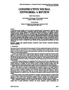
the testing data while using the basic version of the same algorithm. In addition, the respective computational costs of the algorithms while training for different problems are given in Table 2. The average numbers of hidden units and MFLOPS (millions of floating point operations) that were needed for the results in Table 1 are shown. For the readers’ convenience, the best results of all the problems in Tables 1 and 2 are shown in ‘bold’ for both the FSI and the basic versions among all the algorithms. In case of many equal best results in one problem, all of the best results of that particular problem are given in ‘bold’. Figure 1 depicts an example of the behaviour of the objective function values during the training of the first five hidden units with the basic and FSI versions of the MCC algorithm in Henon problem. From the figure one can observe that the hidden unit training of the FSI version starts and usually ends up with higher objective function values than that of the basic version, as we would expect. The results show that the benefits of FSI can be seen in almost all the cases. The results obtained with the FSI versions of the algorithms stay approximately at the same level when compared to the results obtained with the basic versions of the algorithms. FSI seems to be working better in simpler problems, since the results in Laser problem as well as in some cases in Additive problem have deteriorated. On the other hand, FSI versions work as well as basic versions in Mackey-Glass problem, which is the most difficult problem in our simulations. However, this does not change the fact that the enhancements are at their best in the classification problems that happen to be the easiest problems in our simulations. When considering the total number of hidden units needed in the networks, we can see the obvious advantages of our initialization method. Only in Spiral and Laser problems we need to spend regularly more hidden units with the FSI versions than with the basic versions. In most of the cases we are able to use from 20% to 50% less hidden units in the FSI versions than what is needed in the basic versions. One reason for the smaller amount of the hidden units is that we usually end up in higher objective function values in the hidden unit training when we are using appropriate initial values for the network weights thus enabling more efficient hidden unit training. Clearly, as the single hidden units can learn more efficiently, we need a smaller amount of them in the final network to perform the desired overall function.

When comparing the FSI versions of the algorithms to their basic versions one-by-one, we notice that FSI works best with CC, MCC, and FCE algorithms. For CAS and especially for CN the FSI approach is not as successful as we would think beforehand. One reason may be the objective function used in the hidden unit training (which is also used in selecting the best candidate in FSI), since for CAS and CN methods this is a squared error function, while for the other methods it is a maximizable correlation-type function. Another reason for the poor performance of CN is the missing separate output unit. The last hidden unit can not operate as an output unit as efficiently as a separate output unit (which is found in all the other algorithms) can work.

4 Conclusions We presented a forward selection initialization method for some cascade-correlation type constructive neural network algorithms. The key idea of the method is to use a large pool of randomly initialized candidate units, and then to choose the best one of them (according to some predefined criterion which in our simulations was the objective function used in the hidden unit training) to be trained and installed in the active network. The simulations showed that FSI produced equal results with smaller number of hidden units when compared to the basic versions (that use only single randomly initialized candidate hidden units) of the same algorithms.

References: [1] S. E. Fahlman and C. Lebiere, “The Cascade-Correlation Learning Architecture”, Technical Report CMU-CS-90-100, School of Computer Science, Carnegie Mellon University, Pittsburgh, PA, 1990. [2] T.-Y. Kwok and D.-Y. Yeung, “Objective Functions for Training New Hidden Units in Constructive Neural Networks”, IEEE Transactions on Neural Networks, Vol. 8, No. 5, Sep. 1997, pp. 1131-1148. [3] J. Lahnajärvi, M. Lehtokangas, and J. Saarinen, “Fixed Cascade Error - A Novel Constructive Neural Network for Structure Learning”, Proceedings of the Artificial Neural Networks in Engineering Conference, ANNIE’99, St. Louis, Missouri, USA, Nov. 7-10, 1999, pp. 25-30. [4] M. Lehtokangas, J. Saarinen, P. Huuhtanen, and K. Kaski, “Initializing Weights of a Multilayer

Perceptron Network by Using the Orthogonal Least Squares Algorithm”, Neural Computation, Vol. 7, No. 5, 1995, pp. 982-999. [5] M. Lehtokangas, “Fast Initialization for CascadeCorrelation Learning”, IEEE Transactions on Neural Networks, Vol. 10, No. 2, Mar. 1999, pp. 410-414. [6] E. Littmann and H. Ritter, “Generalization Abilities of Cascade Network Architectures”, S. J. Hanson, J. D. Cowan, and C. L. Giles (eds.), Advances in Neural Information Processing Systems, Morgan Kaufman, San Mateo, CA, Vol. 5, 1993, pp. 188-195. [7] Oregon Graduate Institute of Science and Technology, Data Distribution WWW site (http:// www.ece.ogi.edu/~ericwan/data.html).

[8] L. Prechelt, “PROBEN1 - A Set of Neural Network Benchmark Problems and Benchmarking Rules”, Technical Report 21/94, Fakultät für Informatik, Universität Karlsruhe, D-76128 Karlsruhe, Germany, Sep. 1994. [9] L. Prechelt, “Investigation of the CasCor Family of Learning Algorithms”, Neural Networks, Vol. 10, No. 5, 1997, pp. 885-896. [10] M. Riedmiller and H. Braun, “A Direct Adaptive Method for Faster Backpropagation Learning: The RPROP Algorithm”, Proceedings of the IEEE International Conference on Neural Networks, San Francisco, CA, Mar. 28 - Apr. 1, 1993, pp. 586-591. [11] The Santa Fe Time Series Competition Data WWW site (http://www.stern.nyu.edu/~aweigend/ Time-Series/SantaFe.html).

Table 1. Results of the algorithms with all simulation problems. Problems marked with an asterisk (*) give CERR values and the others give NMSE values. The upper values are for the FSI versions and the lower values are for the basic versions of the algorithms. The results are average values of twenty runs. There were no testing data for Chess and Spiral problems, so the values are from training data. In all other cases, the values are from testing data. Algorithm/ Problem

CC

MCC

CAS

CN

FCE

Chess*

0 0

0 0

0 0

0 0

0 0

Spiral*

0 0

0 0

0 0

0.1255 0.1196

0 0

Parity*

0.0806 0.0958

0.0896 0.1042

0.1562 0.0944

0.2980 0.3764

0.0916 0.1225

Cancer*

0.0213 0.0212

0.0208 0.0219

0.0183 0.0231

0.0272 0.0246

0.0222 0.0222

Henon

0.0464 0.0397

0.0432 0.0475

0.0348 0.0460

0.1054 0.0949

0.0501 0.0457

Laser

0.0404 0.0327

0.0425 0.0318

0.0438 0.0288

0.1737 0.1861

0.0389 0.0328

Additive

0.0895 0.0736

0.0670 0.0724

0.0804 0.0683

0.5545 0.5632

0.0939 0.0627

Mackey-Glass

0.3319 0.3252

0.3256 0.3316

0.3247 0.3367

0.4027 0.4060

0.3314 0.3296

(a)

25

25

Training curve of hidden units, MCC:FSI

20

Value of the objective function

Value of the objective function

20

15

10

5

0

(b)

Training curve of hidden units, MCC:basic

15

10

5

0

50

100

150 200 Number of epochs

250

300

350

0

0

50

100

150

200 250 Number of epochs

300

350

Figure 1. (a) The values of the objective function during the training of the first five hidden units with the basic version of the MCC algorithm in Henon problem. (b) The values of the objective function during the training of the first five hidden units with the FSI version of the MCC algorithm in Henon problem. Table 2. The computational costs of the algorithms for different problems. The upper values are average numbers of hidden units and MFLOPS (separated by a semicolon) spent in the FSI versions while the lower values give the corresponding values for the basic versions of the algorithms. The values correspond to the networks that produced the results shown in Table 1. Algorithm/ Problem

CC

MCC

CAS

CN

FCE

Chess

2.90; 0.18 6.70; 0.38

3.10; 0.17 5.75; 0.28

3.85; 0.37 5.80; 0.65

9.15; 0.90 21.25; 2.0

3.00; 0.16 6.90; 0.35

Spiral

42.20; 140 27.75; 50

44.90; 150 30.40; 57

58.35; 370 26.75; 100

74.95; 370 60.65; 130

44.40; 150 31.80; 65

Parity

10.05; 51 10.65; 50

11.05; 58 9.25; 40

11.10; 95 9.45; 100

9.95; 62 12.20; 47

9.15; 44 10.85; 48

Cancer

3.00; 8.3 4.00; 8.7

3.30; 8.8 2.90; 5.8

4.00; 19 3.00; 16

12.40; 68 9.35; 30

2.60; 6.6 2.95; 5.9

Henon

10.55; 7.4 11.45; 5.9

10.00; 6.3 10.85; 5.1

11.15; 11 10.40; 13

21.40; 25 12.25; 6.9

10.30; 6.5 11.60; 5.6

Laser

25.15; 390 19.80; 210

22.85; 330 19.60; 200

35.20; 990 19.75; 470

10.05; 140 10.85; 120

24.60; 370 20.25; 210

Additive

17.45; 62 21.30; 69

17.35; 60 22.15; 75

26.60; 170 20.00; 130

58.40; 420 46.20; 180

18.10; 63 22.50; 70

Mackey-Glass

6.20; 18 10.30; 27

6.75; 20 7.80; 18

9.65; 48 8.85; 45

10.60; 36 7.45; 12

7.80; 25 10.05; 25

400