Constructive Representation of Heterogeneous ... - Semantic Scholar

Constructive Representation of Heterogeneous Objects Ki-Hoon Shin Debasish Dutta Department of Mechanical Engineering, University of Michigan, Ann Arbor, MI 48109-2125

1

This paper proposes a constructive representation scheme for heterogeneous objects (or FGMs). In particular, this scheme focuses on the construction of complicated heterogeneous objects, guaranteeing desired material continuities at all the interfaces. In order to create various types of heterogeneous primitives, we first describe methods for specifying material composition functions such as geometry-independent, geometry-dependent functions, and multiple sets of these functions. Constructive Material Composition (CMC) and corresponding heterogeneous Boolean Operators (e.g., material union, difference, intersection, and partition) are then proposed to illustrate how material continuities are dealt with. Finally, we will describe the model hierarchy and data structure for computer representation. Even though the constructive representation alone is sufficient for modeling heterogeneous objects, the proposed scheme pursues a hybrid representation between decomposition and construction. That is because hybrid representation can avoid unnecessary growth of binary trees. 关DOI: 10.1115/1.1403448兴

Introduction

Conventional solid modeling methods have focused on developing models of physical objects to capture their geometry and topology. Thus far, these approaches have been sufficient, since most physical objects found in engineering applications are homogeneous and manufacturing applications require us to deal primarily with their geometry. Two recent advances, structural optimization 关1,2兴 and Layered Manufacturing 关3兴, enable the design and fabrication of components whose material composition can be controlled and continuously varied along with the geometry. In particular, Layered Manufacturing 共LM兲 or Solid Freeform Fabrication 共SFF兲 techniques have shown much potential for the fabrication of high performance artifacts 共e.g., high-temperature turbine blades or piston heads, injection molding tools with cooling channels, smart structures and mechanisms兲. Composition control is necessary for improving a variety of issues such as thermomechanical performance, increasing toughness and strength, reducing interfacial stresses between materials, limiting crack propagation, and minimizing weight of structural elements 共e.g., plane body, wing兲 being used in aerospace applications without reducing their desirable strength. Just as current solid modelers generate data to drive CNC machines, we expect that the data to drive LM machines will also be generated automatically from future CAD models. This necessitates the capture of material 共composition and gradation兲 information within a solid model. We refer to such an enriched solid model as a ‘‘Heterogeneous Solid Model 共HSM兲.’’ Thus far, heterogeneous objects have been rare in man-made products, but abundant in nature. As pointed out earlier, it becomes possible to build such a heterogeneous object by employing LM technologies. It is also possible to embed components such as sensors, actuators, and microprocessors to create complete assemblies 关4兴. Figure 1 shows such an example, a prototype of the biomechanical arm where there exist local variations in strength, flexibility, and damping. This prototype has two flexible joints, each of which imitates a shoulder and an elbow of the human arm, respectively. The desired material attributes may be obtained by mixing various polymers at different volume fractions during deposition. Since current solid models cannot intrinsically represent this example that has attribute information 共such as material, physical Contributed by the Computer-Aided Product Development Committee for publication in the JOURNAL OF COMPUTING AND INFORMATION SCIENCE IN ENGINEERING. Manuscript received November 2000; revised June 2001. Associate Editor: S. Szykman.

properties, etc.兲 along with the geometry, new modeling systems must be explored. The availability of such modeling techniques remains central to the design, analysis, and fabrication of heterogeneous objects. In this sense, this paper is focusing on the representation schemes of heterogeneous objects. 1.1 Prior Work. Jackson et al. 关5兴 proposed a tetrahedron mesh-based model. Each tetrahedron references four nodes. Each node maintains information about its position in space as well as an associated composition. Jackson 关6兴 also proposed a generalized cellular decomposition method. The interior of the object is decomposed into simpler sub-regions, each of which references information about the composition variation over its domain. The regions of graded composition are general tensor product Bezier volumes. Similar to the tetrahedron model, Kumar and Wood 关7兴 presented a two-dimensional mesh-based model represented by fournode iso-parametric quadrilateral elements. The material composition within each element is represented by interpolating nodal values with iso-parametric shape functions for the four-node quadrilateral element. Wu et al. 关8兴 proposed a NURBS-based Volume model. An object is represented in a hybrid model including a NURBS representation and a voxel-based model. A voxel object can be generated through voxelization of its NURBS volume that is a generalization of NURBS representation of curves and surfaces. Park et al. 关9兴 also proposed a volumetric multi-texturing method for Functionally Graded Material 共FGM兲 representation. Kumar and Dutta 关10,11兴 proposed the r m -object model. This modeling scheme is basically an extension of solid modeling to handle heterogeneous objects by using r-sets 关12,13兴 as the basis of representing the geometry, with material information. Different material regions within an object can be represented in the manner of interior decomposition. A set of Boolean operators 共union, intersection, and difference兲 was also proposed to construct complicated r m -objects. To represent this biomechanical arm, finite element-based representations like 关5,7兴 and voxel-based representations like 关8兴 first require mesh generation and voxelization, respectively. However, the main limitations are inaccuracy in both geometry and material representation, due to the finite approximation of continuous properties and large storage requirement. On the other hand, decomposition methods proposed in 关6,11兴 need to decompose the interior into several simpler sub-regions. Thus, those methods possibly generate redundant entities 共e.g., vertices, edges,

Journal of Computing and Information Science in Engineering Copyright © 2001 by ASME

SEPTEMBER 2001, Vol. 1 Õ 205

2

Heterogeneous Primitive Sets „hp-sets…

Constructive representations of heterogeneous objects are ordered binary trees whose leaf nodes are heterogeneous primitive sets 共hp-sets兲; thus, an hp-set is the smallest component of a heterogeneous object. In the mathematical sense, an hp-set is defined as a subset (G,M (G)) of the product space T⫽E3 ⫻Rn where G傺E3 is an r-set and M共G兲傺Rn is the image set of the material mapping M. An hp-set is thus equivalent to an r m -set. However, the basic properties of the hp-set are quite different from those of the r m -set. The following sections describe in detail the basic properties of the hp-set that are newly derived to support the creation of various types of hp-sets. Fig. 1 A prototype of the biomechanical arm

and faces兲 at the interfaces and it may become an issue how to guarantee desired material continuity at the interfaces. 1.2 Constructive Representation. Considering the difficulties of existing representation schemes, the constructive representation may be advantageous for modeling heterogeneous objects. The CSG representation in solid modeling defines complex solids as compositions of simpler solids; thus boundaries of joined components need not match and interiors need not be disjoint. In this sense, this paper introduces a new, enhanced representation scheme for heterogeneous objects based on the constructive representation. In particular, the new scheme focuses on the construction of complicated heterogeneous parts guaranteeing desired material continuities at all the interfaces. Resulting material continuity depends on the designer’s intent and can mean either no continuity 共for homogeneous lumps of dissimilar materials兲 or higher order continuity for graded materials. The constructive representation always retains all the information of heterogeneous models involved in the construction tree so that it is possible to detect and solve any material discontinuity problem occurring at the interfaces. Similar to CSG representation in solid modeling, complex heterogeneous models are defined as compositions of simpler heterogeneous models, thus the constructive representation of heterogeneous objects requires: • Creating heterogeneous primitives • Heterogeneous modeling operators 共geometry operators and material operators兲 • New model hierarchy and data structure The constructive representation developed in this paper basically has been built upon the work by 关11兴. In principle, the basic concepts of the r m -set and r m -object in 关11兴 are comprehensive, thus they may be used to define heterogeneous primitives 共or objects兲 in most representation schemes such as voxel-based, finite mesh-based, and decomposition models. In this sense, a heterogeneous primitive set 共hp-set兲 and a generalized heterogeneous object 共h-object兲 being defined in this paper are equivalent to an r m -set and an r m -object, respectively. However, the main properties are much different from those of r m -set and r m -object. Furthermore, a new terminology, ‘‘heterogeneous Boolean set 共hb-set兲’’ will be defined to support the constructive representation. The details of these heterogeneous entities 共hp-set, hb-set, and h-object兲 will be discussed later. The remainder of this paper is structured as follows. In section 2, we first describe the heterogeneous primitive set newly defined in this paper. Sections 3 and 4 then describe in detail methods for creating heterogeneous primitive sets and constructing complicated heterogeneous objects. Next, section 5 presents the model hierarchy and data structure required for computer representation. Section 6 gives two specific examples, one of which is a prototype of the biomechanical arm shown in Fig. 1. Finally, section 7 presents a brief summary. 206 Õ Vol. 1, SEPTEMBER 2001

2.1 Modeling Space for hp-sets. Heterogeneous objects are composed of different constituent materials called primary materials. At any given geometric point in the heterogeneous object, the material is a combination of the primary materials and is specified by the volume fraction of each of the n primary materials. Hence, the heterogeneous modeling space is represented by the product space T⫽E3⫻Rn where Euclidean space E3 and Rn represent the geometry space and material space, respectively. In the material space Rn, each dimension represents the volume fraction of a primary material. The physical material space will be restricted due to the fact that the sum of the volume fractions of the primary materials should be unity. Thus the physical material space V共傺Rn兲 has n⫺1 degrees of freedom and can be defined as:

再

V⫽ vគ 苸Rn兩储 vគ 储 1 ⬅

n

兺 ␯ ⫽1 i⫽1

i

and ␯ i ⭓0

冎

(1)

where 储 vគ 储 1 denotes the L 1 -norm, n is the number of primary materials, and v i is the volume fraction of the ith primary material. Figure 2共a兲 shows that the geometric point xគ is associated with its corresponding material point vគ by a composite mapping M that consists of three component mappings such as T, F, and H. In fact, the composite mapping M is a set of material composition functions, each of which maps a geometric point to the corresponding dimension of a material point. However, it is likely to be difficult for a designer to define n material composition functions directly on the geometric space. In contrast, dealing with F instead of M may be easier because the actual material variation is more likely to be defined on the parameter space rather than geometry space. From now on, we will consider F as a set of material composition functions and the parameter space as material function coordinates. In addition, we define two material spaces, namely the customized material space and the primary material space. Each customized material becomes any combination of primary materials just as a painter creates his own color on the palette by mixing primary colors. Using the customized material space, the number of material composition functions to be defined in a set can be reduced to just two in most cases. For instance, to represent a linear material variation of n primary materials between r⫽r a and r⫽r b in cylindrical coordinates, it is necessary to define (n⫺1) material composition functions ( f 1 , . . . , f n⫺1 ) as shown in Fig. 2共b兲. In contrast, only one material composition function g 1 is required if two customized materials 共m គ 1 ,m គ 2兲 are being introduced. vគ (r a ) and vគ (r b ) are volume fraction vectors at r⫽r a and r⫽r b , respectively. Each dimension 共a 1 , . . . ,a n , b 1 , . . . ,b n 兲 of vគ represents the volume fraction of a primary material. First, a material function coordinate transform T maps a geometric point xគ to a parametric point uគ . This is a one to one mapping from E3 to Rdim( uគ ) and is given by: T:E3 →R គ dim共 uគ 兲兩 T共 xគ 苸E3兲 ⬅uគ ⫽ 兵 u i 其

(2)

The dimension of parameter space dim(u) is determined by the Transactions of the ASME

Fig. 3 Effective material function domain

and

គ 1m គ2 ...m គ k兴⫽ 关 m兴 ⫽ 关 m

Fig. 2 A heterogeneous modeling space for cylindrical material coordinates

number of parameters appearing in the material composition functions. For the cylindrical material coordinates shown in Fig. 2, T and dim(uគ ) are defined as: T共 xគ 兲 ⫽

冋冑

x 2 ⫹y 2 ,tan⫺1

冉冊册

y ,z ⫽ 关 r, ␪ ,z 兴 ⫽uគ and dim共 uគ 兲 ⭐3 x (3)

Then, a set of material composition functions F maps a parametric point uគ to a customized material point vគ c . This is also a one to one mapping from Rdim( uគ ) to Vc(傺Rk) as follows. F:R

→Vc兩储 F共 uគ 兲储 1 ⬅

兺 f 共 uគ 兲 ⫽1 i

i⫽1

where F共 uគ 兲 ⬅vគ c ⫽ 兵 c i 其 (4)

where k is the number of customized materials and c i is the volume fraction of the ith customized material. Finally, the material space transform H maps a customized material point vគ c to a primary material point vគ . This is a one-to-one mapping from Vc(傺Rk) to V共傺Rn兲 and is given by: n

H:Vc→V兩储 H共 vគ c 兲储 1 ⬅

兺 h 共 vគ 兲 ⫽1 i⫽1

i

c

where H共 vគ c 兲 ⬅vគ ⫽ 兵 ␯ i 其 (5)

In fact, the material space transform H can be described by an n ⫻k matrix formed as follows. vគ ⫽H共 vគ c 兲 ⫽ 关 m兴 •vគ c where vគ ⫽ 关 ␯ 1 ␯ 2 . . . ␯ n 兴 T ,

vគ c ⫽ 关 c 1 c 2 . . . c k 兴 T

(6)

m 12

...

m 1k

m 21

m 22

...

m 2k

...

...

...

...

m n1

m n2

...

m nk

册

where m គ i 傺V(i⫽1, . . . ,k) represents the ith customized material in terms of n primary materials. 2.2 Effective Material Function Domain „D…. As mentioned above, a set of material composition functions F is defined as a mapping from the parameter space Rdim( uគ ) to the customized material space Rk. To facilitate the design process of F, we introduce the concept of an effective material function domain 共D兲. Thus, F is now defined only within its effective function domain. The function value whose parameter is outside D is determined by the condition satisfying C 0 continuity of the material composition functions. This effective function domain 共D兲 is defined as the intersection of three distinct domains, geometric (D g ), functional (D f ), and user-defined domain (D u ), as follows. D⫽D g 艚D f 艚D u where D傺Rdim共 uគ 兲

k

dim共 uគ 兲

冋

m 11

(7)

The geometry domain (D g ) is automatically determined because F is only valid within its corresponding geometry. The functional domain (D f ) is derived from the fact that the function values of component functions ( f 1 , . . . , f n ) are only valid between 0 and 1, and the sum of these values should be unity. By introducing a user-defined domain (D u ), the designer can selectively define F as parts of original continuous functions without using discrete design techniques 共e.g., f 1 ⫽0.2 for r⬍0.2, f 1 ⫽r for 0.2⭐r ⬍0.8, f 1 ⫽0.8 for r⭓0.8兲. Figure 3 describes this concept for a simple FGM cylinder, គ 2 兲 and its which consists of two customized materials 共m គ 1 and m material composition varies along the radius 共F⫽ 关 f 1 , f 2 兴 T, f 1 (r)⫽r, f 2 (r)⫽1⫺r兲. Each of the three cases shows a completely different distribution of material m គ 1 even though they have the same material composition functions that are C ⬁ continuous. Figures 3共a, b, c兲 show the f 1 (r) trimmed by its own geometric domain (0.4⭐r⭐1.2), functional domain guaranteeing valid volume fractions (0.0⭐r⭐1.0), and user-defined domain (0.2⭐r ⭐0.8) that is optional, respectively. Thus, the final effective function domain becomes (0.4⭐r⭐0.8) and the range of volume frac-

Journal of Computing and Information Science in Engineering


Table 1 Basic properties of the hp-set

sets of material composition functions to be defined over the same geometry. This new capability will be discussed in section 3.5 in detail.

3 Methods for Creating Material Composition of hp-sets As mentioned earlier, the material mapping M of an hp-set consists of a material function coordinate transform T, a set of material composition functions F, and a material space transform H. Among the three component mappings, choosing an appropriate T is the main part of creating hp-sets, since it determines the types of material composition functions, thus governing the overall material distribution over the hp-set. Several types of material composition functions have been developed in this paper as follows: • Geometry-independent functions 共Cartesian, cylindrical, and spherical coordinates兲 • Distance-based functions • Blending functions • Sweeping functions • Multiple sets of above-described functions The following sections describe methods for creating hp-sets in the context of specific applications. For these applications, the material distribution of each hp-set is assumed to be optimized and so its desired material variation is already known.

tion of m គ 1 becomes 0.4⭐ v f ⭐0.8 as shown in Fig. 3共d兲. ⳵ D L and R ⳵ D represent the domain left limit 共DLL兲 and the domain right limit 共DRL兲 of the effective function domain D, respectively. In general, an effective function domain consists of subeffective domains; thus D is given in terms of DLLs and DRLs as follows. D⫽艛 i 关 ⳵ D L i , ⳵ D R i 兴 where i is finite

(8) ⬁

Employing the effective material function domain, the C continuous function changes into a C 0 continuous material composition function over the geometry. C 0 continuity is a sufficient condition for one-to-one mapping. Thus, material composition functions defined in an hp-set should be at least C 0 continuous. In general, C 0 continuity can be considered as smooth grading unless the interval of domain is too small since the actual manufacturing resolution is limited and the requirement of continuity depends on the specific application. If higher than C 0 continuity is required, a simple blending at both discontinuity points can be used. Table 1 summarizes the basic properties of the hp-set newly defined in this paper. An hp-set can now represent a partial FGM region over its geometry without decomposition and approximate a distinct material 共DM兲 region by defining an FGM region whose domain interval 共␧兲 is sufficiently small. It also allows multiple

3.1 Geometry-Independent Composition Functions. This type of function is defined by choosing an appropriate coordinate type 共Cartesian, cylindrical, or spherical兲 and coordinate system 共global, local, or user-defined兲 that defines the origin and orientation of triads. The material composition functions are thus independently defined from the geometry of hp-sets. However, the main application is for designing an hp-set that has exact geometry or an axisymmetric model like a flywheel in which the choice of coordinate system is obvious. In general, using this type of function is very efficient since the evaluation of volume fractions is much faster and more accurate. Figure 4共a兲 shows a composite layer whose material function is periodic in Cartesian coordinates. This object can be directly fabricated by LM machine if its deposition direction is chosen to be parallel to the material variation direction. On the other hand, many application parts have circular profiles as their cross sections, such as the part shown in Fig. 4共b兲. Assuming the pressure vessel is subjected to a high temperature/pressure on the inside, it is desirable to have ceramic on the inner surface 共due to its good high temperature properties兲 while it is also desirable to have metal away from the inner surface 共due to its good mechanical properties兲. Joining the two materials 共metal and ceramic兲 abruptly will lead to high stresses or delamination at the interface. Therefore, an FGM design is required for its inner boundary. A ball joint sliding part shown in Fig. 4共c兲 may improve its friction wear resistance by FGM design.

Fig. 4 Geometry-independent material functions

208 Õ Vol. 1, SEPTEMBER 2001

Transactions of the ASME

Fig. 6 Angular blending Fig. 5 Distance-based material functions

3.2 Distance-Based Functions From Reference Entities. This type of function is useful in designing an hp-set that has a thin-coated layer over geometric boundaries. The user needs to choose a set of reference entities 共e.g., vertices, edges, faces, shells, and lumps兲 and then define k⫺1 distance-based functions for k customized materials. A distance function defined with reference to a vertex 共or a line兲 is equivalent to a spherical 共or cylindrical兲 coordinate function. The dimension of the material function coordinates is 1 and its variables are defined as: dim共 uគ 兲 ⫽1 and uគ ⫽ 关 u 1 兴 where u 1 ⫽min共 d 1 , . . . ,d i , . . . ,d e 兲 (9) where d i is the minimum distance between the geometric point xគ and ith entity, and e is the number of reference entities. Many algorithms are now available for minimum distance calculation. Liu et al. 关14兴 developed an efficient distance algorithm based on preprocessing the model with bucket sorting and digital distance transform. As shown in Fig. 5共a兲, a piston head 关15兴, a thin coat of zirconia is sprayed upon a steel substrate for thermal protection of the upper face and for friction wear protection of the side-faces. Figure 5共b兲 shows another example of a turbine blade that has a thin ceramic coat over the metal. The thin ceramic coat can improve its heat resistance and anti-oxidation properties on the hightemperature environment. This technique is also applicable to many structural elements used in aerospace applications 共e.g., turbine blades, vanes, plane body, etc.兲 that are subject to severe thermomechanical loading giving rise to intense thermal stresses. 3.3 Blending Composition Functions. This type of function is useful in modeling an intermediate FGM region between several separated entities 共e.g., vertex, edges, faces兲 whose geometries are arbitrary and disconnected from one another. Assuming that each entity represents one customized material, p customized materials assigned to p separated regions are blended smoothly. The following sections describe two blending methods. Angular Blending. Angular blending uses the distance ratio (u 1 ⫽d 2 /(d 1 ⫹d 2 )) as the blending coordinate. To calculate two distance variables 共d 1 and d 2 兲, it uses ray-casting and twodimensional intersection algorithms. This method is good for blending an intermediate region between two non-concave boundaries that are generally concentric. However, this method is not applicable if there are more than two blending entities. Figure 6 shows an example that consists of two customized materials 共m គ 1 and m គ 2 兲, each of which is assigned to the outer and inner boundary, respectively. In fact, this example represents the cross section of the cooling channels embedded in the mold assembly. The details of this example will be presented in the section 3.4. Inverse Distance (R-function) Blending. Using inverse distance weighting 关16 –18兴, a material composition vគ c can be con-

structed as a linear combination of the material composition vector m គ i 共the ith customized material兲 assigned to the ith geometric boundary ( ⳵ B i ) with weight functions w i . The weighting functions w i are constructed by normalizing each inverse distance. Therefore, w i are inversely proportional to the distance d i (xគ ) from the ith geometric boundary where material composition is m គ i . In addition, the weight functions w i are positive continuous functions satisfying the interpolation condition w i ( ⳵ B j )⫽ ␦ i j and forming a partition of unity. Thus, the inverse distance blending is formulated as: p

vគ c 共 xគ 兲 ⫽

兺 mគ •w 共 xគ 兲 i

i⫽1

i

where p

w i 共 xគ 兲 ⫽

兿

␮

j⫽1,j⫽i

d j j 共 xគ 兲

p

p

兺兿

k⫽1 j⫽1,j⫽k

␮

d j j 共 xគ 兲

and p

兺 w 共 xគ 兲 ⫽1 i⫽1

i

(10)

where d i (xគ ) is distance from point xគ to the ith geometric boundary ( ⳵ B i ), p is the number of geometric boundaries and the exponents ( ␮ i ) control behavior of the weight functions. Based on this formulation, the material function coordinates are defined as (u 1 , . . . ,u p ) and are exactly equivalent to the weight functions (w i , . . . ,w p ). Thus, the dimension of the material function coordinates is p and its variables are defined as: dim共 uគ 兲 ⫽p and uគ ⫽ 关 u 1 ,u 2 , . . . ,u p 兴 ⫽inverse – distance – blending共 d 1 ,d 2 , . . . ,d p 兲 (11) where d i is the minimum distance between the geometric point xគ and ith set of reference entities, and p is the number of sets of reference entities. Figure 7 shows an example that has three closed loops. Three blending coordinates 共u 1 , u 2 , and u 3 兲 are computed by expanding Eq. 共10兲 with p⫽3. As an hp-set constructed by using inverse distance blending, Fig. 8 shows the overall procedures for modeling a simple mold with a cavity. Figure 8共a兲 shows how to define the inner and outer boundaries that limit the blending region. The inner and outer boundaries are classified by the parting surface marked by grids. The inner boundaries determine the shape of the cavity and the outer boundaries control the FGM thickness in the x, y, and z directions. In general, bulk properties such as volume contraction are dependent on overall dimensions, and the boundary conditions can be varied according to where the maximum heat flux occurs and so on. Thus, this method can give the designer good flexibility



Fig. 7 Material function coordinates in inverse distance blending

for varying the thickness of an FGM layer directionally 共e.g., t x , t y , and t z 兲. Figure 8共b兲 shows the material distribution over the mold assembly. Replacing the distance function (d(xគ )) by the constructed R-function 关18,19兴, the above-described inverse distance formula becomes the inverse R-function formula. In general, inverse R-function blending can guarantee better smoothness 共or differential properties兲. However, the constructed R-function is not an exact distance function, thus it seems to be difficult for a designer to predict overall material distribution and control it exactly. An example using inverse R-function blending will be presented in section 3.4. For details on R-function theory, refer to 关18,19兴. 3.4 Sweeping Composition Functions. This type of function is suitable for representing an hp-set whose geometry is created by sweeping a cross section along an arbitrary path. The designer draws a cross section and its sweeping path on the twodimensional plane and then defines a set of material composition functions. Figure 9 shows the material coordinate transform T in sweeping coordinates. The first component T 1 maps the geometric point xគ into xគ ⬘ . The y ⬘ axis is perpendicular to the sweeping plane where the sweeping path lies, and the z ⬘ axis is defined along the sweeping path so that z ⬘ coordinate is equivalent to the chord-length from the sweeping origin. Similar to the geometry-independent function coordinates, the second component T 2 mapping xគ ⬘ into uគ is again classified into sweep-Cartesian, sweep-cylindrical, and sweep-two-dimensional – blending coordinate transforms. Sweep-Two-Dimensional – Blending Composition Functions. This type of function is suitable for representing a swept hp-set whose material composition varies over the sweeping cross section and needs to be blended by several material boundaries. Applying blending methods discussed in section 3.3 to the twodimensional sweeping cross section, over the intermediate region several material boundaries are blended smoothly without any abrupt joint.

Fig. 8 A simple mold created by a blending function


In this sense, the cooling channel of the mold is a good example to which sweep-two-dimensional – blending can be applied. In general, cooling channels are required to regulate the heat transfer rate from the die to the coolant without reducing the overall strength of the die. For this purpose, H13 steel is widely used as the die material, with copper as the material of cooling channels. The cores 共or cavities兲 of the mold are cooled in the conventional manner by running a series of long longitudinal holes horizontally through the mold that are connected together on the outside by plastic tubing. Thus far, machining has been the only way to embed cooling channels inside a die. Employing LM techniques, a die with embedded cooling channels can be fabricated directly, which are conformable to the mold cores 共or cavities兲. Figures 10共a, b, c兲 show three different types of material distributions over the cross section of cooling channels, each of which is respectively constructed by angular blending, inverse distance blending, and inverse R-function blending discussed in section 3.3. Figures 11共a, b兲 show a mold assembly embedding conformable cooling channels and its material distribution, respectively. Note, the outer boundary of the cross section is used to create the material distribution and is not an actual geometric boundary. In other words, the outer boundary will be merged into the mold assembly, as shown in Fig. 11共b兲. 3.5 Supporting Multiple Sets of Material Composition Functions in an hp-set. An hp-set allows multiple sets of material composition functions to be defined over the same geometry. With this new capability, most FGM parts can be described by a single hp-set without applying Boolean operations, thereby reduc-

Fig. 9 Material coordinate transform for sweeping functions

Transactions of the ASME

Fig. 10 Material distribution on the cross section of the cooling channel

ing the depth of constructive representation. For this purpose, the overall mapping 共M兲 from a geometric point xគ into a material point vគ is finally defined as logical disjunction 共∨兲 of submappings (M i ). M⫽∨ i Mi ⫽∨ i 共 Hi •Fi •Ti 兲

i⫽1, . . . ,s

where M:E →V兩 M共 xគ 苸E 兲 ⬅vគ ⫽ 兵 ␯ i 其 3

3

(12)

where s is the number of sets of material composition functions defined in an hp-set. However, each set of material composition functions has an effect on the material composition of geometric points (xគ ) whose material function coordinates (T(xគ )) lie in its effective function domain 共D兲. That is, interference regions between any two inverse images Ti⫺1 (Di ) and T⫺1 j (D j ) 共defined in E3 兲 of effective function domains D i and D j 共defined in Rdim( uគ ) 兲 are not permissible. This constraint can be formulated as follows: Ti⫺1 共 Di 兲艚T ⫺1 j 共 D j 兲 ⫽⌽ i⫽ j, 1⭐i, j⭐s

(13)

Thus, the actual evaluation of material composition corresponding to the geometric point xគ can be described as follows: If xគ 苸G and Ti 共 xគ 兲苸Di then vគ c 共 xគ 兲 ⫽Fi 共 Ti 共 xគ 兲兲

(14)

Else if xគ 苸G and Ti 共 xគ 兲苸Di for all i⫽1, . . . ,s then vគ c 共 xគ 兲 ⫽vគ mc where vគ mc ⫽matl – continuity共 F1 共 ⳵ DL1 兲 ,F1 共 ⳵ DR1 兲 , . . . ,Fs 共 ⳵ DsL 兲 ,Fs 共 ⳵ DsR 兲兲 where ⳵ DiL and ⳵ DiR represent the domain left limit 共DLL兲 and the domain right limit 共DRL兲 of the ith effective function domain (D i ), respectively 共we assume that there is only one effective function domain for each set of material composition functions F兲. vគ mc is chosen to satisfy at least C 0 material continuity among

Fig. 11 Mold assembly embedding conformable cooling channels

volume fraction vectors (Fi ( ⳵ DiL ),F i ( ⳵ DiR )) evaluated at all domain limits. Due to this constraint, the usage of this method is quite limited. Figure 12 shows an hp-set where two sets of material composition functions 共M 1 and M 2 兲 are defined in terms of three customized materials A 共Blue兲, B 共Green兲, and C 共Red兲. Since three test points a, c, and e are outside the effective function domains 共D 1 and D 2 兲, their volume fractions are evaluated using domain limits that satisfy material continuity condition. For instance, vគ c (c) should be F1 ( ⳵ DR1 )⫽F2 ( ⳵ DL2 ) to guarantee material continuity. The basic principle for this ‘‘matl – continuity’’ function is that no evaluation occurs across the effective function domains 共D 1 and D 2 兲, i.e., vគ c (c) can be neither F1 ( ⳵ DL1 ) nor F2 ( ⳵ DR2 ) because it crosses D 1 共or D 2 兲 to be F1 ( ⳵ DL1 ) 共or F2 ( ⳵ DR2 )兲.

4 Modeling Operators for Constructing Heterogeneous Objects The designer can now construct complicated heterogeneous primitives by applying heterogeneous Boolean operators between two hp-sets. Similar to CSG representation in solid modeling, the newly created heterogeneous primitive can be used for the synthesis of more complicated heterogeneous primitives. One advantage of using the constructive representation is that it provides the designer with an easier way to model and modify heterogeneous objects. Most modern CSG solid modeling systems rely on a hybrid representation of solids 共mixed between B-rep and CSG兲 since CSG lacks the capability to perform local operations such as blending and tweaking, which are typical operations in B-rep based solid modeling systems. Furthermore, as Boolean steps grow, the traversal of the binary tree becomes increasingly computationally intensive, thus often resulting in long updates for minor changes. Therefore, the proposed scheme in this paper is also based on the hybrid representation. The geometry of each node 共leaf, internal, and root兲 is maintained as a B-rep and the material composition is constructed by the binary tree structure. 4.1 Heterogeneous Boolean Set „hb-set…. While constructing a complicated heterogeneous primitive, the most important issue is how to blend more than two materials smoothly at the interfaces. The Boolean operators proposed in 关11兴 are mainly developed for the design of distinct material regions, thus inadequate for the design of FGM parts. That is because they do not consider the degree of continuity at the interfaces and the resultant geometry has to be decomposed into two or three disjoint subregions. This may propagate numerical errors as Boolean steps increase due to the redundancy of geometric boundaries at the interfaces. To solve these problems, we now define a heterogeneous Boolean set 共hb-set兲 as a Boolean construction of two heterogeneous primitives. An hb-set consists of the resultant geometry and the Constructive Material Composition 共CMC兲 that is a binary tree



Fig. 12 Multiple sets of material composition functions

constructed from two heterogeneous primitives. The CMC of the hb-set is thus completely different from the material mapping M of the heterogeneous primitive set 共hp-set兲. More specially, CMC is composed of a specific Boolean operator 共e.g., material union, intersection, difference, or partition兲, the original data of the two heterogeneous primitives and blending information at the interfaces. The blending information includes the weight factor for the intersection region and distance-based boundary blending functions. Using this information stored in CMC, the material composition can be uniquely evaluated at any given point over the resultant geometry 共Q兲. An hb-set B is given by: B⫽共Q,C兲⫽ 共 Geometry共 B兲 ,Material共 B兲兲

(15)

where ␾ ij is the jth component function of the ith material mapping and n is the number of primary materials available in the material library. The material Boolean operator (M 1 丣 M 2 ) is defined as logical disjunction 共⵪兲 of three component operators (M 1and2 ,M 1out2 ,M 2out1). ␣ is a constant weight factor for the intersection region and w i (i⫽1,2) is the ith boundary blending function whose argument is d i , the distance from the ith boundary. Similar to material composition functions, w i is only defined between 0 and 1. In particular, the material Boolean operator 共丣兲 is consistently applicable to other modeling operations such as material intersection, difference, and partition. More specifically, the three components of the material operator 共丣兲 are defined as follows:

3

where Q傺E is an r-set and C共Q兲債V is the image set of the constructive material composition C. In this sense, an hb-set is another type of r m -set as the hp-set. As mentioned earlier, however, there is no requirement of material continuity for an hb-set because Boolean operations can be performed without material blending at the interfaces of the two low-level primitives. This property is the main difference between the hp-set and the hb-set, even though an hb-set can be treated as a new heterogeneous primitive like an hp-set. Handling Material Continuity in hb-sets. Based on this definition, Fig. 13 shows three different hb-sets that are constructed by a heterogeneous UNION operation between two hp-sets. This also describes how the CMC is constructed and how it guarantees desired material continuity at the interfaces. All three cases generate a smooth joining of two hp-sets, which are more likely to correspond to the original design intent. In particular, case 3 creates a new material property for the intersection region, which is very useful when imposing new material properties on a local part of the given geometry. In Fig. 13, G i and M i represent the geometry and material mapping of the ith hp-set, respectively. Each material mapping for n primary materials is defined as: M1⫽H1•F1•T1⫽ 兵 ␾ 11 , ␾ 12 , . . . , ␾ 1n 其 M2⫽H2•F2•T2⫽ 兵 ␾ 21 , ␾ 22 , . . . , ␾ 2n 其 212 Õ Vol. 1, SEPTEMBER 2001

(16)

M1and2⫽ ␣ •M1共 xគ 兲 ⫹ 共 1⫺ ␣ 兲 •M2共 xគ 兲 for xគ 苸共 G1 艚 * G2兲 , 0⭐ ␣ 共 ⫽const 兲 ⭐1

(17)

M1out2⫽w 2 •M1共 xគ 兲 ⫹ 共 1⫺w 2 兲 • ⳵ M2共 xគ ⬘ 兲 for xគ 苸共 G1⫺ * G2兲 , 0⭐w 2 ⫽w 2 共 d 2 兲 ⭐1 M2out1⫽ 共 1⫺w 1 兲 • ⳵ M1共 xគ ⬘ 兲 ⫹w 1 •M2共 xគ 兲 for xគ 苸共 G2⫺ * G1兲 , 0⭐w 1 ⫽w 1 共 d 1 兲 ⭐1 where ⳵ M i (i⫽1,2) denotes the material composition at the point xគ ⬘ that lies on the ith geometric boundary of the intersection region and is closest to the query point xគ . Modeling Operations for hp-sets. The following operations can be classified by their geometric operations. There is no difference between material operations dealing with material information 共i.e. material operator is consistently applicable regardless of geometric operators.兲 • Union Operation: The following material operation 共丣兲 for union is the same as defined in Fig. 13. Transactions of the ASME

Fig. 13 Three different hb-sets constructed by a material union operation

* 共 G2 ,M2兲 ⫽ 共 G1艛 * G2 ,M1 丣 M2兲共 G1 ,M1兲艛 m ⫽ 共 G1艛 * G2 ,M1and2∨M1out2∨M2out1兲 (18) • Intersection Operation:

* 共 G2 ,M2兲 ⫽ 共 G1艚 * G2 ,M1 丣 M2兲 ⫽ 共 G1艚 * G2 ,M1and2兲共 G1 ,M1兲艚 m (19) • Difference Operation:

* 共 G2 ,M2兲 ⫽ 共 G1⫺ * G2 ,M1 丣 M2兲 ⫽ 共 G1⫺ * G2 ,M1out2兲共 G1 ,M1兲 ⫺ m (20) • Partition Operation: This operation is only valid for heterogeneous objects, and is very useful for imposing a new material property on a local part of the given geometry.

4.2 Generalized Heterogeneous Object „h-object…. The generalized heterogeneous object 共h-object兲 is the generic name for representing heterogeneous solid models. Even though the constructive representation alone is sufficient for modeling h-objects, the proposed scheme pursues a hybrid representation between decomposition and construction, i.e., an hb-set is defined only if necessary. That is because hybrid representation can avoid unnecessary growth of binary trees. In order to take advantage of the benefits of both representations, we finally define an h-object O as a finite collection of hp-sets and hb-sets; thus, an h-object can be classified as an r m -object as mentioned earlier. Each hp-set and hb-set belonging to the same h-object is geometrically interior-disjoint to the others as follows. O⫽兵P1 , . . . ,Pa ,B1 , . . . ,Bb其 where a and b are finite ⫽ 兵共 G1 ,M1兲 , . . . , 共 Ga ,Ma兲 , 共 Q1 ,C1兲 , . . . , 共 Qb ,Cb兲其

* 共 G2 ,M2兲 ⫽ 共 G1 ,M1 丣 M2兲 ⫽ 共 G1 ,M1and2∨M1out2兲共 G1 ,M1兲 / m (21) Figure 14 shows the results of material intersection, difference, and partition between two primitives shown in Fig. 13. In particular, Fig. 14共b兲 shows that the difference operation is useful for creating thin FGM layer.

Gi 艚 * Gj⫽⌽ i ⫽ j,

1⭐i, j⭐a

Qi艚 * Qj⫽⌽ i ⫽ j,

1⭐i, j⭐b

Gi 艚 * Qj⫽⌽ 1⭐i⭐a,

(22)

1⭐ j⭐b

where P and B represent an hp-set and an hb-set, respectively. 4.3 Modeling Operations for h-objects. As mentioned earlier, an hp-set, an hb-set, or a collection of these can form an h-object. Thus, modeling operations defined for hp-sets are now generalized to h-objects. Material Union, Intersection, Difference, and Partition for h-objects. Those modeling operations are now defined between two h-objects and still create an hb-set. Based on the operations for hp-sets, the actual Boolean operations for h-objects are equivalent to the following internal sub-operations: O1⫽兵P11 , . . . ,P1a ,B11 , . . . ,B1b其 Fig. 14 Material intersection, difference, and partition

O2⫽兵P21 , . . . ,P2c ,B21 , . . . ,B2d其 where a, b, c, and d are finite



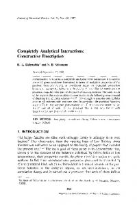
algorithms. Note that the root h-object can be constructed by applying five UNION operations without decomposition. As shown in Fig. 15, an hb-set is defined as a Boolean construction between two low level primitives 共two h-objects兲. The dotted lines between an hb-set and two children h-objects imply that the material composition of the hb-set will always refer to the material compositions of two children and the blending information at the interfaces. Note, the two children h-objects are not actual parts of their parent hb-set, i.e., the two children h-objects are not geometrically interior-disjoint. In contrast, an hp-set 共or an hb-set兲 is always a part of its parent h-object. This property is the primary distinction of an hb-set from an h-object. 5.2

Fig. 15 Model hierarchy in the constructive representation

O1共 Operation兲 O2

⫽∨ i, j

冦

P1i 共 Operation兲 P2 j

1⭐i⭐a,1⭐ j⭐c

P1i 共 Operation兲 B2 j

1⭐i⭐a,1⭐ j⭐d

B1i 共 Operation兲 P2 j

1⭐i⭐b,1⭐ j⭐c

B1i 共 Operation兲 B2 j

1⭐i⭐b,1⭐ j⭐d

冧 (23)

Join Operation. In addition to the basic Boolean operations, the current system uses a special operation called Join, which updates the linked list of hp-sets or hb-sets. In particular, this operation is very useful when it is obvious that there is no geometric intersection 共i.e., disjoint兲 and no continuity requirement between two entities 共e.g., an hb-set and an h-object, an hb-set and an h-object兲. This operation adds a new hp-set or hb-set to the original linked list of hp-sets or hb-sets. In fact, this operation is developed to support the decomposition representation explicitly. This operator also reduces the depth of the CMC tree, which is the most important role of this operator in constructive representation. The join operation between two h-objects is defined as: O1∨O2⫽O3 ⫽兵P11 , . . . ,P1a ,P21 , . . . ,P2c ,B11 , . . . ,B1b ,B21 , . . . ,B2d其 ⫽ 兵 P31 , . . . ,P3共a⫹c兲 ,B31 , . . . ,B3共b⫹d兲其

(24)

In the resultant h-object O3, if the two material mappings M i and M j of two hp-sets P i and P j are identical, two hp-sets are combined into a single hp-set. The join operation between two hp-sets is defined as: Pi ∨P j ⫽ 共 Gi ,Mi 兲 ∨ 共 G j ,M j 兲 i⫽ j ⫽

5

冉

共 Gi 艛 * G j ,Mi 兲

if Mi ⫽M j

兵共 Gi ,Mi 兲 , 共 G j ,M j 兲其

if Mi ⫽M j

冊

(25)

Model Hierarchy and Data Structure

5.1 Model Hierarchy. Figure 15 shows an h-object satisfying these definitions. The root h-object consists of one hp-set and two hb-sets, each of which is constructed by a UNION operation between two sub-h-objects. In fact, the evaluation of material composition corresponding to an arbitrary geometric point is based on the six leaf primitives 共hp-sets兲 by recursive descent 214 Õ Vol. 1, SEPTEMBER 2001

Data Structure for Computer Representation

Data Structure for the hp-set. Figure 16 shows the implemented data structure for an hp-set in this paper. This data structure was derived from the commercial ACIS geometric modeler 共Spatial Technology, Inc.兲关20兴 that is based on the well-known radial-edge data structure 关21兴 that is widely adopted as the modeling kernel within various solid modeling systems. The radialedge data structure provides a unified method for representing solid models. The data structure maintains the topology of the models in terms of the different topological entities such as BODY, LUMP, SHELL, FACE, LOOP, EDGE, and VERTEX. A material related data structure 共MATL兲 equivalent to the material mapping M is then added to the original data structure as shown on the right. To allow multiple sets of material composition functions over the same geometry, MATLs are linked to each other. Two types of material composition function are available, such as analytic functions and b-spline curves. Each material function is directly parsed to evaluate volume fractions corresponding to the parametric values 共i.e., physical coordinates for geometry-independent functions, blending coordinates or distance from reference geometry兲. Data Structure for an h-object. As mentioned earlier, an h-object 共Fig. 17兲 is a finite collection of hp-sets and hb-sets and the hp-sets 共or hb-sets兲 are linked to each other to represent decomposed parts of the h-object. An hb-set stores a constant weight factor for the intersection region, specified Boolean operation type, and new resultant geometry, as well as two sets of h-objects and their blending functions. In particular, the blend function is defined in terms of the minimum distance from the geometric boundary of each h-object.

6

Examples

In this paper, a prototype Heterogeneous Solid Modeler 关22兴 has been implemented. More specifically, the heterogeneous solid modeler using the h-object framework is implemented in C⫹⫹ using the ACIS kernel and the GUI is implemented using Motif and OpenGL libraries. The GUI is necessary for high-level interaction between the user and the heterogeneous CAD system. The geometry and material distribution functions are input by the user to the heterogeneous solid model. This section presents two examples constructed by CMC modeling. 6.1 A Prototype of the Biomechanical Arm. Figure 18 shows the overall modeling procedure for a prototype of the biomechanical arm previously shown in Fig. 1. In general, the FGM design for a joint can improve damping characteristics and fatigue resistance, thus each joint requires a graded region between stiff and soft materials to give the desired flexibility and strength. For this example, the final object can be created by two union operations of three heterogeneous primitive sets. In particular, even though the original material for G 3out共12兲 is M 3out共12兲共yellow material兲, it becomes ⳵ M 12 共red material兲 if d 2 is greater than 6(w 2 ⫽0). 6.2 Piston With Zirconia Coating and MMC Crown. Figure 19 shows a heterogeneous piston with Metal Matrix ComposTransactions of the ASME

Fig. 16 Data structure representing an hp-set

Fig. 17 Data structure representing an h-object



Fig. 18 Construction of the biomechanical arm

ite 共MMC兲 crown and its model hierarchy. One of the important applications of MMCs in the automotive area is in diesel piston crowns 关23兴. This application involves incorporation of short fibers of alumina or alumina⫹silica in the crown of the piston. The product with the MMC crown becomes much lighter, more abrasion resistant, and cheaper. The final piston model can be constructed by material partition between two primitives. In particular, the piston primitive has an FGM layer of zirconia over steel substrate for thermal protection as already shown in Fig. 5共a兲.

Fig. 19 Piston head with Metal Matrix Composite „MMC…


In Fig. 19, d 1 is defined as minimum distance from the boundaries of G 2 . The final model clearly shows that the CMC method guarantees desired material continuity at the interfaces between zirconia⫹steel and MMC.

7

Summary

In this paper, several representation schemes for heterogeneous objects 共or FGMs兲 have been briefly reviewed. A new representation scheme called ‘‘constructive representation’’ and the corresponding data structure are then proposed. In general, many updates 共or modifications兲 of original models occur at the design stage. Therefore, the constructive representation is advantageous especially in model construction and modification, storage requirement, and material interrogation accuracy when compared to other approaches such as finite-element-based, voxel-based, and decomposition methods. Furthermore, the proposed CMC operators can guarantee desired material continuities at all the interfaces while constructing complicated heterogeneous objects. However, material blending at the interfaces may be valid only if the materials involved are dissolved into the stable state of each other, a topic of continuing research in material science. Another issue in the design of FGM parts is how to represent material information, specifically material composition functions within heterogeneous primitives. Several approaches based on Bezier/NURB blending functions have been proposed so far in 关6,8兴. However, the main difficulty of these approaches is that their construction procedures are not well defined and do not correspond to the designer’s intuition. In this paper, several methods using geometry-independent, geometry-dependent functions, and multiple sets of material composition functions have been proposed. However, those capabilities are not yet enough to model arbitrary material distribution as represented by CT or MRI images. Thus, more work has to be done in specifying material composition of heterogeneous primitives. In engineering applications, the main need for heterogeneous object modeling is to design material and shape optimized objects. Hence a mesh generation algorithm for FE analysis is a critical factor and the development of adaptive mesh generation algorithms based on the material distribution is a topic for further research. Transactions of the ASME

Acknowledgments The authors gratefully acknowledge the financial support from NSF grant MIP-9714951 for this research.

References 关1兴 Bendsoe, M., and Kikuchi, N., 1988, ‘‘Generating Optimal Topologies in Structural Design Using a Homogenization Method,’’ Comput. Methods Appl. Mech. Eng., 71, pp. 197–224. 关2兴 Cherkaev, A., 1994, ‘‘Relaxation of Problems of Optimal Structural Design,’’ Int. J. Solids Struct., 31, No. 16, pp. 2251–2280. 关3兴 Ashley, S., 1991, ‘‘Rapid Prototyping Systems,’’ Mech. Eng. 共Am. Soc. Mech. Eng.兲, pp. 34 – 43. 关4兴 Rajagopalan, S., Goldman, R., Shin, K. H., Kumar, V., Cutkosky, M., and Dutta, D., 2001, ‘‘Representation of Heterogeneous Objects During Design, Processing and Freeform-Fabrication,’’ Mater. Des., 22, No. 3, pp. 185–197. 关5兴 Jackson, T. R., Liu, H., Patrikalakis, N. M., Sachs, E. M., and Cima, M. J., 1999, ‘‘Modeling and Designing Functionally Graded Material Components for Fabrication With Local Composition Control,’’ Mater. Des., 20, No. 2/3, pp. 63–75. 关6兴 Jackson, T., 2000, ‘‘Analysis of Functionally Graded Material Representation Methods,’’ Ph.D. thesis, Massachusetts Institute of Technology, Cambridge, MA. 关7兴 Kumar, V. Ashok, and Wood, Aaron, 1999, ‘‘Representation and Design of Heterogeneous Components,’’ Proc. SFF Conference, Austin, TX. 关8兴 Wu, Zhongke, Seah, Hock Soon, and Lin, Feng, 1999, ‘‘NURBS-Based Volume Modeling,’’ Proc. Int. Workshop on Volume Graphics, Swansea, pp. 321– 330. 关9兴 Park, S. M., Crawford R. H., and Beaman, J. J., 2000, ‘‘Functionally Gradient Material Representation by Volumetric Multi-Texturing for Solid Freeform Fabrication,’’ presented at the 11th Annual Solid Freeform Fabrication Symposium, Austin, TX. 关10兴 Kumar, V., and Dutta, D., 1998, ‘‘An Approach to Modeling and Representation of Heterogeneous Objects,’’ ASME J. Mech. Des., 120, No. 4, pp. 659– 667.

关11兴 Kumar, V., 1998, ‘‘Solid Modeling and Algorithms for Heterogeneous Objects,’’ Ph.D. Thesis, Department of Mechanical Engineering and Applied Mechanics, University of Michigan, Ann Arbor, MI. 关12兴 Requicha, A., 1980, ‘‘Representation for Rigid Solids: Theory, Methods and Systems,’’ Computing Surveys, 12, No. 4. 关13兴 Hoffman, C., 1989, Geometric & Solid Modeling, Morgan Kaufmann Publishers. 关14兴 Liu, H., Cho, W., Jackson, T. R., Patrikalakis, N. M., and Sachs, E. M., 2000, ‘‘Algorithms for Design and Interrogation of Functionally Gradient Material Objects,’’ Proc. ASME 26th Design Automation Conference, Baltimore, MD, Paper No. DETC2000/DAC-14278. 关15兴 Suresh, S., and Mortensen, A., 1997, ‘‘Functionally Graded Metals and MetalCeramic Composites: Thermomechanical Behavior,’’ Int. Mater. Rev., 42, No. 3, pp. 85–116. 关16兴 Shepard, D., 1968, ‘‘A Two-Dimensional Interpolation Function for Irregularly Spaced Data,’’ Proc. 23 Nat. Conf. ACM, pp. 517–524. 关17兴 Alfeld, P., 1985, ‘‘Multivariate Perpendicular Interpolation,’’ SIAM 共Soc. Ind. Appl. Math.兲 J. Numer. Anal., 22, pp. 96 –106. 关18兴 Rvachev, V. L., Sheiko, T. I., Shapiro, V., and Tsukanov, I., 2000, ‘‘Transfinite Interpolation Over Implicitly Defined Sets,’’ Technical Report SAL 2000-1, Spatial Automation Lab., Univ. of Wisconsin. 关19兴 Rvachev, V. L., 1967, ‘‘Theory of R-Functions and Some Applications,’’ Naukova Dumka, in Russian. 关20兴 ACIS Geometric Modeler: Application Guide, 1995, Spatial Technology Inc. 关21兴 Weiler, K. J., 1986, ‘‘The Radial Edge Structure: A Topological Representation for Non-Manifold Geometric Modeling,’’ in: M. J. Wozny, H. McLaughlin, and J. Encarnacao, eds., Geometric Modeling for CAD Applications, Elsevier Science Publishers, Holland, pp. 3–36. 关22兴 Bhashyam, S., Shin, K. H., and Dutta, D., 2000, ‘‘An Integrated CAD System for Design of Heterogeneous Objects,’’ Rapid Prototyping J., 6, No. 2, pp. 119–135. 关23兴 Donomoto T., Miura N., Funatani K., and Miyake N., 1983, SAE Tech. Paper No. 83052, Detroit, MI.

