Transmit Power Estimation with a Single Monitor in Multi-band Networks Shaxun Chen†, Kai Zeng‡, Ningning Cheng†, Prasant Mohapatra† Department of Computer Science, University of California, Davis, CA 95616 ‡ Department of Computer and Information Science, University of Michigan, Dearborn, MI 48128
[email protected],
[email protected],
[email protected],
[email protected] †
Abstract— Transmit power estimation is widely used in network monitoring, power-aware design of MANETs, primary user detection in cognitive radio networks and many other areas. Traditional methods for transmit power estimation are trilateration-based, which require an underlying infrastructure with at least three monitors. In this paper, we propose a novel transmit power estimation method which utilizes the nuance of the received signal strength at different frequencies. Our method only needs one monitor, thus has less hardware requirement and is much easier to carry around. We use a support vector machine to facilitate the estimation, and conduct real-world experiments to validate our method. The experimental results demonstrate that our method is able to achieve the accuracy as high as 90%, which in practice outperforms the trilateration method using multiple monitors. Keywords: transmit power estimation; multi-band transmitter;
support vector machine; support vector regression. I.
INTRODUCTION
In wireless networks, transmit power is an important attribute of wireless signal. Transmit power estimation is required or helpful in multiple areas. In wireless sensor networks, transmit power estimation is used to infer the working status and battery life of sensor nodes. In cognitive radio networks, it helps in detecting the presence of primary users [1]. In mobile ad-hoc networks, estimation of transmit power supports power-aware operations, such as power- aware routing, media access control, etc. In addition, in wireless networks, every node should follow the FCC’s regulation and transmit under a certain power limit; otherwise, excessive interference or even jamming attack occurs, which prevents other nodes from communicating. Transmit power estimation can be applied to detect such malicious behaviors. In order to estimate the transmit power, monitor(s) measures the received power strength of the signal from the transmitter. In many cases, the location of the transmitter is unknown, such as a newly joined sensor, a legacy primary user or a node in a mobile ad-hoc network. Without the distance information, the estimation of transmit power is a non-trivial task. The existing solutions are based on the trilateration method. More than three monitors are required for transmit power estimation [1]–[5]. These monitors should be deployed beforehand
and located far away from each other in order to achieve acceptable performance. In such methods, deploying monitors and collecting data introduces high overhead. When the target is not in the coverage of the underlying monitor infrastructure, power estimation fails. In this paper, we propose a novel transmit power estimation method which only needs a single monitor. Our method is applicable to multi-band transmitters. Nowadays, many wireless devices can work in multiple bands. Most cell phones are tri-band or quad-band (850/900/1800/1900MHz); 802.11n network cards work on both 2.4GHz and 5GHz bands. Moreover, cognitive radio is emerged as the future paradigm of wireless communication, which typically has a wide frequency band. For instance, USRP with SBX daughterboard covers the band from 400MHz to 4.4GHz. It is foreseeable that more and more wireless devices will become multi-band-capable. Our method captures the nuance of the received signal strength when the transmitter transmits at different bands, and then makes use of it to reversely infer the transmit power using a support vector machine. Since only one monitor is needed, our method is much more convenient compared with the traditional methods. The user can even carry the monitor, and perform the estimation wherever he/she likes. To the best of our knowledge, this is the first work that estimates the transmit power with a single monitor when the location of the transmitter is unknown. We conduct extensive real-world experiments to evaluate the effectiveness of our method. The result demonstrates that our method is able to achieve an estimation accuracy of as high as 90% with a relatively small training set. In practice, it outperforms trilateration based method using multiple monitors. The remainder of this paper is organized as follows. Section Ⅱdiscusses related work. Section Ⅲ states the problem. In Section Ⅳ we introduce our method for transmit power estimation. Section Ⅴ evaluates our work. Section Ⅵ discusses several related issues, and Section Ⅶ concludes the paper. II.
RELATED WORK
Both theoretical and empirical models have been developed in the past decades to depict the signal attenuation, including log-normal, log-distance, Okumura model, etc. Given received signal strength and the distance from the transmitter, transmit power can be reversely inferred using these models. But without the distance information, we cannot perform estimation
solely depending on them. Kim, et al. [1] proposed a trilateration based method to localize the primary user and estimate its transmit power in cognitive radio networks. A propagation model with log-normal path loss is assumed. At least four monitors are needed to measure the received signal strength from different directions. The measurements are then gathered together to calculate the transmit power. Ho, et al. [2] studied the estimation of transmit power in MANETs utilizing geometric constraints. Different from [1], they allow using only two or three monitors, but the output is the lower bound of the transmit power. Zafer, et al. proposed a similar method, but additionally took the influence of channel fading (log-normal fading) into account [3] [4]. They pointed out that their estimation can converge to the real transmit power as the number of monitors increases. Ho, et al. further extended the work to the case where multiple transmitters coexist [5]. All of these approaches require multiple monitors which are located relatively far away from each other in order to achieve decent performance. In contrast, our method only needs one single monitor for transmit power estimation, which largely reduces monitor deployment overhead and makes our method much easier to conduct. Besides, the studies mentioned above are all theoretical analyses, which have not been tested in the real-world experiments. III.
PROBLEM DEFINITION
We estimate the transmit power of a wireless transmitter based on the received signal strength. The location of the transmitter or the distance between the transmitter and the monitor is unknown. This is a typical scenario we encounter when estimating the transmit power of a remote node. The transmitter is able to transmit in multiple bands (greater than or equal to two). Bands that are significantly separated are preferred. Adjacent or overlapping channels usually cannot be counted as different bands. For example, channel 1 and channel 2 in 802.11 are not considered as two different bands because they are very close to each other (2.412GHz and 2.417GHz). As mentioned in Section Ⅰ, more and more wireless devices will become multi-band-capable, especially when wireless communication shifts to the cognitive radio paradigm, in which transmitters change their transmission frequency dynamically to make better use of the scarce spectrum. Assuming the transmitter has n bands, and we successfully capture its signal in m of these n bands, and the received signal strength from m bands are P1, P2, .., Pm, respectively. Our goal is to determine the transmit power PT of this transmitter. Here we assume the transmitter maintains its transmit power unchanged when it shifts bands. This assumption is valid in most cases. For instance, walkie-talkies do not change their transmit power when switching to another band; 802.11abg cards use the same transmit power in 2.4GHz and 5GHz bands by default. The case where the transmitter changes its power when switching band is planned as a part of our future work.
In order to capture the transmitter’s signal, the monitor should have the same working bands as the transmitter. The monitor switches among its bands quickly in order to obtain more Pi (1 ≤ i ≤ m). Besides random switching, there are also other strategies, such as uncoordinated frequency hopping [6] [7]. How to efficiently capture the wireless signal from a multi-band (or multi-channel) transmitter is well studied in the context of channel (link) rendezvous of frequency hopping or cognitive radio communication [13] [14] [15], which is orthogonal to our research. In the next section, we will focus on how to estimate PT based on the observations P1, P2, .., Pm. IV.
TRANSMIT POWER ESTIMATION WITH SINGLE MONITOR
In this section, we first introduce the basic idea behind our method, and then present the methods of coarse-grained estimation and fine-grained estimation respectively. A. Frequency Affecting Path Loss The RF propagation models depict the attenuation of wireless signals. The free-space propagation model reveals the relationship between received signal strength and distance in a perfect vacuum, which is given as follows. (1) PR = PT·GR·GT / (4d·f)2 where PR is received power, d is the distance between the transmitter and the receiver (monitor), and f is the frequency of the RF signal. GT and GR are transmitting antenna gain and receiving antenna gain, respectively. Let PL be path loss, we have PL = PT/PR, and take logarithm for both sides: (2) PL (dB) = C + 20logd + 20logf Here C is a value depending on antenna gains. From Equation 2 we can see that, for different frequencies, the signal attenuation rates are the same. In other words, when d gets larger, the increment of PL is independent of f. This result is illustrated in Figure 1. As shown in this figure, the attenuation curves of different frequencies are parallel. In this case, measuring received signal strength under multiple frequencies does not help infer the transmit power.
Figure 1. Path loss in free space
Fortunately, the perfect vacuum does not exist in the real world; and as we know, radio waves with higher frequencies tend to be absorbed easier by objects. As a result, high frequency signals attenuate faster than low frequencies, which is why the long distance wireless communication usually uses lower frequency radios. This phenomenon is also described by some propagation models, such as log-distance model and Okumura Model [8]. We will come back to them again a little later in our discussion. Assuming in practice, the path loss under the different frequencies follows the plot in Figure 2, in which higher frequency signal decays faster. Figure 2 is by no means an accurate description of ground truth; we only use it as an illustration to explain the feasibility of our method. Let P1 and P2 be the received signal strength at 300MHz and 3GHz respectively, since the attenuation curves of different frequencies are not parallel now, d (the distance between the transmitter and the monitor) can be determined by |P1-P2| (see Figure 2). Having d and P1 (or P2), it is easy to infer PT.
tenuates faster. But Okumura Model determines A by checking the table or plots; for such models without analytical expressions, it is difficult to calculate PT the same way as in Figure 2. 2) Attenuation curve varies when environment changes. The attenuation curve of RF signal is sensitive to the environment. Buildings, foliages, and even weather conditions can have significant impact on the signal absorption. The log-distance model depicts the path loss of RF signal in indoor or densely populated environments. It is given as follows: (4) PL (dB) = PL0 + 10·log(d / d0) + Xg PL0 is the path loss at the reference distance d0, and is the path loss exponent. Some empirical measurements of are shown in Table 1 [9].
Figure 3. Values of Ain the Okumura Model
Figure 2. Inferring transmit power using received power
Above is only an informal explanation to show why estimating transmit power with only one monitor is possible. For practical transmit power estimation, we cannot simply calculate this way. The reason is as follows: 1) Attenuation curves in real-world scenarios are complex; sometimes even do not have closed forms. The plots in Figure 2 are simplified for illustration purpose. The real curve is much more complex or irregular. For instance, Okumura Model is an empirical model and is one of the most common models for signal prediction in urban areas. It is described as follows: (3) PL (dB) = L(f, d) + A(f, d) – G(hT) – G(hR) – GAREA where L(f, d) is the free space path loss and A(f, d) is the median attenuation in addition to free space path loss. The values of A(f, d) are given by Okumura’s empirical plots, part of which is shown in Figure 3 [8]. In Figure 3, the curve of 100km is much steeper than that of 1km, which equivalently indicates that high frequency RF at-
From Table 1 we can see that this model also reveals the fact that the signal of higher frequency attenuates faster. However, in the question “how fast”, it apparently gives the different result compared to the Okumura Model. Even log-distance model itself exhibits very different attenuation curves when the building type is different. For transmit power estimation, we would have to use one model (or one attenuation curve) for each single different environment, which makes the estimate method not self-contained and cumbersome, not to mention that for many environments, there are even no models having been built to characterize it. TABLE I.
PATH LOSS EXPONENT IN DIFFERENT ENVIRONMENTS
Building Type Office with hard partition Office with soft partition Office with soft partition Textile or chemical Textile or chemical
f
1.5GHz
3.0
900MHz
2.4
1.9GHz
2.6
1.3GHz
2.0
4GHz
2.1
3) Antenna gain is not a constant. Most wireless devices do not change their antennas when
they switch to a new band (or a new channel). For example, 802.11abg wireless cards use the same antenna when they transmit at 2.4GHz and 5GHz. Typically, an antenna will have different gains when it transmits at different frequencies (especially when frequency difference is large). As a result, we cannot simply calculate the transmit power by directly using the method exhibited in Figure 2. Thus, based on these discussions, by measuring received signal strength at different frequencies, estimating the transmit power with a single monitor is possible, but can be hardly achieved by simply exploiting the propagation models. We propose to estimate the transmit power using a support vector machine. Machine learning methods treat the relationship between the input (received power measurements) and output (estimated transmit power) as a black box, which is particularly useful for our problem. Among various machine learning based methods, support vector machine is often reported to have superior performance [10] [11]. B. Coarse-Grained Transmit Power Estimation We divided application scenarios into two categories: coarse-grained estimation and fine-grained estimation. The former is suitable for the cases where the precision requirement is not very high. The output of the coarse-grained estimation is a power range. For example, we want to evaluate a sensor’s battery life remotely by estimating its transmit power. We can divide the sensor’s transmit power into three sub-ranges: high, mid, low, which correspond to three battery status: full, good, dying. Therefore, if estimated transmit power is low, we know it is time to change the battery for the sensor. For coarse-grained estimation, assuming the range of PT is divided into t sub-ranges, labeled as y1, y2, …, yt, respectively (see Figure 4). The input of the support vector machine is the signal strength (P1, P2, …, Pm) measured at m different bands by the monitor. The output is estimated power range Y (Y = y1, y2, …, or yt).
Figure 4. Discretization of transmit power
In a nut shell, support vector machine is a classification tool. In the training phase, it tries to divide different groups of samples apart by a set of hyperplanes, which are carefully constructed and lie in the “middle” of the margin between every pair of groups. In our problem, samples are in the form of (P1, P2, …, Pm, yi), where the first m elements are called attributes and the last is label. Specifically, we only use the samples from the shadowed regions in Figure 4. In power estimation problem, different groups are extracted from a continuous range; leaving a guard band (in Figure 4) helps enhance the discrimination
of the samples. For the simplicity of description, we assume there are only two groups, whose labels are y1 and y2, and we let y1 = 1 and y2 = -1. The cases in which the number of groups is more than two can be solved by applying the following process multiple times (build multiple hyperplanes). The hyperplane that separates the samples from the two groups can be expressed as: (5) W X b 0 Where W and X are both (m+1)-dimensional vectors, b is a real number. X in our case stands for the vector (P1, P2, …, Pm, yi). The dot between W and X is inner product. W determines the slope of the hyperplane. As mentioned, we want the hyperplane in the “middle” of the margin. This problem equals to find a hyperplane lying in the margin with its ǁWǁ minimized. Formally, the problem can be described as minimizing ǁWǁ2/2, subject to: W X j b 1 or W X j b 1 where Xj is the jth training sample. Minimizing ǁWǁ2/2 is equivalent to minimizing ǁWǁ. We use the former for mathematical convenience. The objective function above is equal to: l 1 min max{ || W ||2 j [Y j (W X j b) 1]} W ,b 2 j 1 where are non-negative Lagrange multipliers, Yj is the label of the jth sample, and l is the number of training samples. Now this problem can be solved by the standard quadratic programming. Due to the space limitation, we do not present the details here. After the training phase, the hyperplane(s) that separates different sample groups are constructed. In the estimation phase, the measured received power (P1, P2, …, Pm) is used as input of our support vector machine, and it outputs the label (estimated power range) by judging the relative position between the point P : (P1, P2, …, Pm) and the hyperplane we construct. Our experimental results (see Section Ⅴ) show that our method can achieve high estimation accuracy (90%) with measurements from only three bands (m = 3). C. Fine-Grained Transmit Power Estimation For some applications, a power range is not satisfying enough; more accurate estimation is desired. Such examples include power-aware routing and transmit power control. In this subsection, we will introduce our support vector regression based method for fine-grained transmit power estimation. The input of the algorithm is still the signal strength (P1, P2, …, Pm) measured at m different bands. The output now is a numeric value, noted as f( P ). Support vector regression works similarly as support vector machine. The difference is that the hyperplane is built to approximate all the samples instead of separating them. The hyperplane is defined as follows: (6) f ( P ) W P b
where W’ and P are both m-dimensional vectors, b’ is a real number. P stands for (P1, P2, …, Pm). Since it is highly possible that there does not exist such a hyperplane crossing through all the samples, an error is allowed. But with this relaxation, there can be an infinite number of hyperplanes. Our method looks for the hyperplane lying in the “middle” of the allowed region (this property is referred to as flatness). In order to handle irregular samples, we also allow the distance from samples to the hyperplane to be larger than . The exceeded part is referred to as . The difference is that introduces a penalty while does not (see Figure 5). This problem can be formalized as: l minimize 1 || W ||2 K ( ) j j 2 j 1 Pj b subject to Y j W W Pj b Y j where K is a positive constant, which decides the tradeoff between the flatness of the hyperplane and the amount of extra errors ( and '). P j is the attributes of the jth sample, and Yj is still the label of the jth sample.
Here P is the input of the regression function and P j is the attributes of jth training sample. In this equation, b’ can be calculated by exploiting Karush–Kuhn–Tucker conditions. Details can be found in [12]. In the above discussions, hyperplanes are used to approximate samples. Since in our problem, the relationship between the input ( P ) and output (PT) is not linear, using hypersurface could increase the performance of our method. Therefore, we introduce the kernel tricks. It can be proven that the property of support vector regression still holds if we substitute the inner product in Equation 7 with kernel functions. In practice, we employ Gaussian radial basis function, which is one of the commonly used kernel functions. It is defined as: k (i , j ) exp( || i j ||2 )
where is a positive parameter. We use 1/22 for. The updated regression function is: l 1 (8) f ( P) ( j j ) exp( 2 || Pj P ||2 ) b 2 j 1 In the estimation phase, the measured power at different frequencies ( P ) is input into Equation 8, and f( P ) gives the estimated transmit power. V.
EVALUATIONS
In this section, we conduct real-world experiments to evaluate our methods. For both coarse-grained and fine-grained transmit power estimation, we first test their accuracy and then compare their performance to the traditional trilateration based method. A. Experiment Settings We use HP nc6000 laptops as both the transmitter and the monitor. They are equipped with Athores 802.11abg wireless cards and Madwifi driver. Each nc6000 has two WIFI antennas. We manually disable one of them to eliminate the influence of antenna diversity.
Error committed Figure 5. Error function
The above objective function and constrains is equal to minimizing L, which is called Lagrange function: l l 1 L || W ||2 K ( j j ) ( j j j j ) 2 j 1 j 1 l j ( j Y j W Pj b) j 1
l j ( j y j W Pj b) j 1
where ,’, and ’ are Lagrange multipliers and they are all positive. Minimizing a Lagrangian can be converted to a solvable dual optimization problem. Due to the space limitation, we directly give the derived hyperplane: l (7) f ( P) ( j j ) Pj P b j 1
Figure 6. Experiment scenario
We make use of three different frequencies to train the algorithm and estimate the transmit power unless otherwise specified. They are channel 1 (2.412GHz) of 802.11g, channel 36 (5.18GHz) and 149 (5.745GHz) of 802.11a. Modulation
B. Accuracy of Our Transmit Power Estimation Method We first test the accuracy of the transmit power estimation method we proposed in Section Ⅳ. For the coarse-grained estimation, transmit power is divided into three sub-ranges: [7, 9], [10, 12], and [13, 15] (unit: dBm). They are labeled as H(igh), M(edian), and L(ow) respectively. In the estimation phase, the monitor is placed randomly in the dotted area in Figure 6, and measures the received signal strength at three different bands (see Section ⅤA). Although our samples are collected at A, B and C (see Figure 6), we do not require the monitor to locate at these points in the estimation phase. The location of the monitor is not known by our estimation algorithm. We test 100 times in both daytime and evening. Transmit power is evenly distributed in [7, 15] dBm. If the output label of our method is the same as the ground truth, it is regarded as a correct estimation. The accuracy is calculated by (times of correct estimation) / (total estimation times). 90% 80% 70% 60% 50%
With Guard Band Without Guard Band
40% 30% 20%
45
90
135
180
225
Number of Samples Figure 7. Accuracy of coarse-grained estimation
The result is plotted in Figure 7. The x-axis shows the total number of samples. For example, “180” stands for collecting 60 samples at each point (A, B, and C), and in these 60 samples, 20 are with the label “H”, and the same for “M” and “L”. These samples are collected at different time of a day. We tested two cases, with guard band and without (please refer to Section ⅣA). When without guard band, we use every possible value for training. For example, the samples with label “M” can be collected when the transmitter is tuned to 10, 11, or 12dBm . When guard band is applied, in our case, only 7 and
8dBm are used for label “L”, 11dBm for “M”, and 14, 15dBm for “H”. We can see from the experiment, using guard band leads to much better performance. This is because in our problem, sub-ranges are originally extracted from a continuous range, and the samples within guard bands obscure the boundary of the groups. In both cases, the accuracy grows as the number of samples increases. When the guard band is applied, we can achieve the estimation accuracy as high as 90%. The rest of coarse-grained experiments thereinafter all use guard band unless otherwise specified. 90% 80%
Relative Estimation Error
rates are fixed at 6Mbps to achieve larger transmission range. Transmit power are varied from 7dBm to 15dBm for all tests. Received signal strength is extracted from the radiotap.dbm_ antsignal field and recorded by Wireshark. Measured signal strength is typically an integer falling into [-92, -18]. We perform our experiments in an outdoor open area. The transmitter is placed at T, as shown in Figure 6. The training data are collect at A, B, and C (approximately 25m, 50m, and 80m from T), and then mixed together.
70% 60% 50% 40% 30% 20%
45
90
135
180
225
Number of Samples Figure 8. Accuracy of fine-grained estimation
Next, we test the accuracy of our fine-grained estimation method. As presented in Section ⅣB, the input is the same as coarse-grained estimation, but the output is a numeric value. In the training phase, samples are collected evenly at the transmit power from 7dBm to 15dBm at point A, B, and C. Other settings are the same as the experiment above. The accuracy is evaluated by relative estimation error, which is defined as: | estimated power real power | *100% real power The result of fine-grained estimation is shown in Figure 8. As the number of samples increases, the relative estimation error decreases. With 225 samples, the relative error is only 18.1%, which is useful in practice for most transmit power estimation applications. C. Scalability For the methods that utilize supervised learning, an important question is how often we need to train. In this subsection, we will answer this question for our method. In Figure 9, the triangles indicate the estimation accuracy tested from various direction of the transmitter. We use the same training data as the experiments above (collected from points A, B, and C), but in the estimation phase, the monitors is placed randomly in the whole semicircle area in Figure 6 instead of only the dotted area. As shown in Figure 9, the accuracy is very close to the original result (the result in Section Ⅴ B with guard band, shown as the dotted line in Figure 9). This
test shows that with the training data from only one direction, our method can be used to perform estimation from different directions and locations. 90% 80%
Accuracy
70%
ferent hardware specification (or different model), retraining is necessary. D. Frequency Diversity In this experiment, we only transmit and measure the signal in two bands (channel 1 and 36), and compare to the original result using three bands (1, 36, and 149). The comparison results of coarse-grained estimation and fine-grained estimation are shown in Figure 11 and Figure 12 respectively.
60% 50%
90%
Original performance Different transmitter of the same type Different directions
40%
80% 70%
20%
45
90
135
180
225
Accuracy
30%
Number of Samples
50%
Original performance
40%
Only two bands are used (1 & 36)
30%
Figure 9. Scalability of coarse-grained estimation
The squares in Figure 9 show the performance of our method when the transmitter used in estimation phase is different from the one in training (different individual, the same model). In the estimation phase, we use 3 other HP nc6000 laptops as the transmitter and their results are averaged. From figure 9 we cannot see obvious decrease of estimation accuracy. This experiment implies that for the same type of wireless transmitters, we only need to perform training on one of them. Recall the example in Section ⅣB, we want to estimate the transmit power of the nodes in a sensor network. If all these sensors are of the same model, we can train once and apply our method on all of them. Figure 10 presents the same experiment on the fine-grained estimation method and shows very similar results.
20%
45
70% 60% 50% 40% 30% 20%
135
180
225
Figure 11. Coarse-grained estimation with two bands
The performance drops about 10% to 15% when only using channel 1 and 36. Since our method is based on the path loss difference at multiple frequencies, it is reasonable that measuring at more channels improves the estimation accuracy. On the other hand, when we only use channel 36 and 149, the estimation accuracy becomes too low to be useful (not shown in the figure). This is not surprising, because channel 36 (5.18GHz) and 149 (5.745GHz) are too close to generate sufficient difference for model training. 90%
Original performance
80%
Relative Estimation Error
Original performance Different transmitter of the same type Different directions
90
Number of Samples
90% 80%
60%
Only two bands are used (1 & 36)
70% 60% 50% 40% 30% 20%
45
90
135
180
225
Number of Samples
45
90
135
180
225
Number of Samples
Figure 10. Scalability of fine-grained estimation
Figure 12. Fine-grained estimation with two bands
From this subsection, we can see in our method, the trained model is not device or location specific, and has good reusability. Of course, if the transmitter changes to a device with dif-
This experiment suggests that frequency diversity is important to the performance of our method. More channels and larger frequency difference can both contribute to the estimation
E. Performance Compared to Trilateration Method Now we move on to the performance comparison between our method and the traditional trilateration based method. For trilateration method, following the approach proposed in [1], we use four HP nc6000 laptops located around point T (in Figure 6) as monitors, and assume the path loss exponents for four links are the same (otherwise the equations are not solvable). Four equations are built using the measurements from these four monitors, and we solve the estimation problem by least square method. The results of 100 trials are averaged and shown in Figure 13 (coarse-grained) and Figure 14 (finegrained) respectively. For coarse-grained estimation, output values of the trilateration method are converted to labels before calculating accuracy (values between 6 to 15dBm are converted to L, M, and H respectively; values less than 6dBm are counted as errors). For our method, the cases of 225 samples are plotted. 90% 80% 70% 60% 50%
coarse-grained estimation and fine-grained estimation. The former outputs a label, which indicates a sub-range of the transmit power, while the latter outputs a numeric value. Apparently, converting a numeric value to a label is easy. So theoretically the fine-grained estimation method is able to perform both fine-grained estimation and coarse-grained estimation. It seems that the coarse-grained estimation method is not necessary.
Relative Estimation Error
accuracy. Limited by the hardware ability of our devices (802.11abg cans can only work in 2.4GHz and 5GHz), we utilize at most three bands. It is conceivable that the accuracy of our method can be further improved if measurements in more bands are available. We plan to exploit it using cognitive radio devices in our future work.
Figure 14. Our method (fine-grained) vs. trilateration
In this experiment, we use two methods mentioned above to conduct the coarse-grained transmit power estimation task respectively. The transmit power of the transmitter varies within [7, 15] dBm, which is divided into three sub-ranges (L: [7, 9], M: [10, 12], H: [13, 15]). The coarse-grained estimation method is with the guard bands. The output of the fine-grained method is rounded and then converted to labels. If the result is smaller than 7 or larger than 15, the estimation is counted as an error.
40% 30%
90%
20%
80%
Trilateration 2.4G
Trilateration 5G
Figure 13. Our method (coarse-grained) vs. trilateration
The result shows that in practice, the trilateration method has lower accuracy than our method. The four monitors used in the trilateration method are placed in different locations; they may suffer from different multi-path effect and shadow fading. However, in the trilateration method, the same path loss model and path loss exponent are assumed, which hurts the estimation accuracy. We also find that in 5GHz band the trilateration method has better performance than in 2.4GHz. This may because the latter band suffers more from interference. In this experiment, our method exhibits its significant advantage over the trilateration method in practice. With less number of monitors, we can achieve even better performance than the traditional method. F. Coarse-Grained Estimation vs. Fine-Grained Estimation In Section Ⅳ , we proposed two estimation methods:
70%
Accuracy
Our method
60% 50% 40%
Coarse-grained estimation method with guard band 30%
Fine-grained estimation method with label mapping
20%
45
90
135
180
225
Number of Samples Figure 15. Two methods for coarse-grained estimation
The performance comparison between two methods is plotted in Figure 15. The coarse-grained method outperforms the fine-grained method in power range estimation. When the training set is small, the difference is even larger. This experiment implies that two methods both have their own advantages. The fine-grained method is able to predict the concrete value
while the coarse-grained method is more suitable for range estimation. They cannot substitute each other. VI.
DISCUSSION
As introduced in the previous sections, the advantages of our estimation method include low hardware requirement, less deployment overhead and higher accuracy. In fact, there is another important difference between our method and the traditional methods. As we know, many wireless devices cannot directly report the strength of a received signal; instead, they report RSSI (Received Signal Strength Indicator), which is a positive integer indicating the signal strength. However, the mappings between the RSSI and real signal strength are vendor dependent and usually not publicly available. If such a device is used as the monitor, trilateration based methods cannot work. In contrast, our method still works in this case. Monitors are easier to be qualified for our method. In Section ⅤC, we have mentioned that our method does not need retraining when the monitor’s location changes. However, if the transmitter itself moves to a place with very different surroundings, such as a hilly area, retraining is highly recommended. We also point out that retrain is not necessary for transmitters that are of the same model. But there is a tricky problem. For example, two different laptops use the same wireless card and the same driver, but they can behave very differently. This is because the antenna they use may be different, or the locations where the antenna is installed are different. An antenna located in the upper border of the screen tents to have much higher gain than the same one installed under the keyboard. Therefore, “transmitters of the same model” suggests all parts of the transmitters are identical and the configurations are the same. Our method only needs one monitor, but it does not disallow multiple monitors. If more than one monitor is available, they can be used together to reduce errors. We can also dedicate one monitor to one band, so that it will take less time to gather the measurements at m bands. For our method, even if multiple monitors are used, we do not require them to be located far away to each other, and do not need their geographic coordinates as algorithm input.
support vector machine. Two approaches are developed, in order to deal respectively with the scenarios of low-precision and high-precision requirement. Our methods only need one monitor to perform power estimation, which has much lower costs compared to the traditional methods. We conducted real-world experiments to evaluate the effectiveness of the method we proposed. The result shows that our method can achieve the estimation accuracy as high as 90%. It outperforms the trilateration method which uses three or more monitors. For the future work, we plan to conduct the experiments on a cognitive radio platform. With richer frequency diversity, our method has the potential to further improve power estimation performance. REFERENCES [1] [2] [3] [4]
[5] [6]
[7]
[8]
[9] [10]
[11] [12] [13]
VII. CONCLUSION In this paper, we introduced a novel method for transmit power estimation in multi-band networks. We measure the received signal strength at different bands, and make use of the differences between them to infer the transmit power using a
[14]
[15]
S. Kim, H. Jeon, H. Lee, J.S. Ma, “Robust Transmission Power and Position Estimation in Cognitive Radio,” ICOIN, 2007. I.W. Ho, B.J. Ko, M. Zafer, C. Bisdikian, and K.K. Leung, “Cooperative Transmit-Power Estimation in MANETs,” WCNC, 2008. M. Zafer, B.J. Ko, and I.W. Ho, “Cooperative Transmit-Power Estimation under Wireless Fading,” MobiHoc, 2008. M. Zafer, B.J. Ko, and I.W. Ho, “Transmit Power Estimation using Spatially Diverse Measurements under Wireless Fading,” IEEE/ACM Tran. on Networking, 18(4):1171-1180, 2010. I.W. Ho, B.J. Ko, M. Zafer, “Blind Estimation of Transmit-Power for Multiple Wireless Sources,” Milcom, 2008. M. Strasser, S. Capkun, C. Popper, M. Cagalj, “Jamming-resistant Key Establishment using Uncoordinated Frequency Hopping,” IEEE Symposium on Security and Privacy, pp. 64-78, May 2008. M. Strasser, C. Popper, and S. Capkun, “Efficient Uncoordinated FHSS Anti-jamming Communication,” 10th ACM International Symposium on Mobile Ad Hoc Networking and Computing, pp. 207-218, 2009. Y. Okumura, E. Ohmori, T. Kawano, K. Fukuda, “Field Strength and its Variability in VHF and UHF Land-Mobile Radio Service,” Review of Elec. Comm. Lab., Vol 16, No.9-10 pp.825-873, 1968. J.S. Seybold, “Introduction to RF Propagation,” Wiley Press, 2005. N.I. Sapankevych, R. Sankar, “Time Series Prediction using Support Vector Machines: A Survey,” IEEE Computational Intelligence Magazine, pp. 24-38, May 2009. C. Burges, “A Tutorial on Support Vector Machines for Pattern Recognition,” Data Mining and Knowledge Discovery, 2(2): 121-167, 1998. A.J. Smola, B. Scholkopf, “A Tutorial on Support Vector Regression,” Statistics and Computing, Springer, 2004. Z.L. Lin, H. Liu, X. Chu, and L. Yiu-Wing, “Jump-Stay based Channel-Hopping Algorithm with Guaranteed Rendezvous for Cognitive Radio Networks,” IEEE Infocom, 2011. Y. Zhang, Q. Li, G. Yu, and B. Wang, “Etch: Efficient Channel Hopping for Communication Rendezvous in Dynamic Spectrum Access Networks,” IEEE Infocom, 2011. N. Theis, R. Thomas, and L. DaSilva, “Rendezvous for Cognitive Radios,” IEEE Tran. on Mobile Computing., (10)2: 216-227, 2011.