They also describe an extension to the AdaBoost algorithm that boosts this objective function. .... fbis (TREC-5), la1 (Los Angeles Times), hitech (San Jose.
Proceedings of the IEEE International Conference on Data Mining, 2004.
Multi-View Clustering Steffen Bickel and Tobias Scheffer Humboldt-Universit¨at zu Berlin Department of Computer Science Unter den Linden 6, 10099 Berlin, Germany {bickel, scheffer}@informatik.hu-berlin.de
Abstract We consider clustering problems in which the available attributes can be split into two independent subsets, such that either subset suffices for learning. Example applications of this multi-view setting include clustering of web pages which have an intrinsic view (the pages themselves) and an extrinsic view (e.g., anchor texts of inbound hyperlinks); multi-view learning has so far been studied in the context of classification. We develop and study partitioning and agglomerative, hierarchical multi-view clustering algorithms for text data. We find empirically that the multiview versions of k-Means and EM greatly improve on their single-view counterparts. By contrast, we obtain negative results for agglomerative hierarchical multi-view clustering. Our analysis explains this surprising phenomenon.
1. Introduction In some interesting application domains, instances are represented by attributes that can naturally be split into two subsets, either of which suffices for learning. A prominent example are web pages, which can be classified based on their content as well as based on the anchor texts of inbound hyperlinks; other examples include collections of research papers. If few labeled examples and, in addition, unlabeled data are available, then the co-training algorithm [4] and other multi-view classification algorithms [15, 5] improve the classification accuracy often substantially. Multi-view algorithms train two independent hypotheses which bootstrap by providing each other with labels for the unlabeled data. The training algorithms tend to maximize the agreement between the two independent hypotheses. Dasgupta et al. [7] have shown that the disagreement between two independent hypotheses is an upper bound on the error rate of one hypothesis; this observation explains at least some of the often remarkable success of multiview learning. It also gives rise to the question whether
the multi-view approach can be used to improve clustering algorithms. Partitioning methods – such as k-Means, k-Medoids, and EM – and hierarchical, agglomerative methods [11] are among the clustering approaches most frequently used in data mining. We study multi-view versions of these families of algorithms for document clustering. The rest of this paper is organized as follows. We review related work in Section 2, the problem setting and evaluation issues in Section 3. We discuss partitioning multiview clustering algorithms in Section 4 and hierarchical algorithms in Section 5. Section 6 concludes.
2. Related Work Research on multi-view learning in the semi-supervised setting has been introduced by two papers, Yarowsky [18] and Blum and Mitchell [4]. Yarowsky describes an algorithm for word sense disambiguation. It uses a classifier based on the local context of a word (view one) and a second classifier using the senses of other occurrences of that word in the same document (view two), where both classifiers iteratively bootstrap each other. Blum and Mitchell introduce the term co-training as a general term for bootstrapping procedures in which two hypotheses are trained on distinct views. They describe a cotraining algorithm which augments the training set of two classifiers with the np positive and nn negative highest confidence examples from the unlabeled data in each iteration for each view. The two classifiers work on different views and a new training example is exclusively based on the decision of one classifier. Blum and Mitchell require a conditional independence assumption of the views and give an intuitive explanation on why their algorithm works, in terms of maximizing agreement on unlabeled data. They also state that the Yarowsky algorithm falls under the co-training setting. The co-EM algorithm [16, 10, 5] is a multi-view version of the Expectation Maximization algorithm for semi-supervised learning.
Collins and Singer [6] suggest a modification of the cotraining algorithm which explicitly optimizes an objective function that measures the degree of agreement between the rules in different views. They also describe an extension to the AdaBoost algorithm that boosts this objective function. Dasgupta et al. [7] give PAC bounds for the generalization error of co-training in terms of the agreement rate of hypotheses in two independent views. This also justifies the Collins and Singer approach of directly optimizing the agreement rate of classifiers over the different views. Clustering algorithms can be divided into two categories [3]: generative (or model-based) approaches and discriminative (or similarity-based) approaches. Model-based approaches attempt to learn generative models from the documents, with each model representing one cluster. Usually generative clustering approaches are based on the Expectation Maximization (EM) [8] algorithm. The EM algorithm is an iterative statistical technique for maximum likelihood estimation in settings with incomplete data. Given a model of data generation, and data with some missing values, EM will locally maximize the likelihood of the model parameters and give estimates for the missing values. Similarity-based clustering approaches optimize an objective function that involve the pairwise document similarities, aiming at maximizing the average similarities within clusters and minimize the average similarities between clusters. Most of the similarity based clustering algorithms follow the hierarchical agglomerative approach [11], where a dendrogram is build up by iteratively merging closest examples/clusters. Related clustering algorithms that work in a multi-view setting include reinforcement clustering [17] and a multiview version of DBSCAN [12].
3. Problem Setting and Evaluation We consider the problem that data is generated by a mixture model. Without knowing the true parameters of the mixture model, we want to estimate parameters of mixture components and thereby cluster the data into subsets so that with high probability two examples that are generated by the same mixture component get assigned to the same cluster, and examples generated by different components get assigned to different clusters. We consider the special case of a multi-view setting, where the available attributes V of examples are split into disjoint sets V (1) and V (2) . An instance x is decomposed and viewed as (x(1) , x(2) ), where x(1) and x(2) are vectors over the attributes V (1) and V (2) , respectively. These views have to satisfy the conditional independence assumption. Definition 1 Views V (1) and V (2) are conditionally independent given a mixture component y, when ∀x(1) ∈
V (1) , x(2) ∈ V (2) : p(x(1) , x(2) |y) = p(x(1) |y)p(x(2) |y). To measure the quality of a clustering, we use the average entropy over all clusters (Equation 1). It is based on the impurity of a cluster given the true mixture components of the data. pij is the proportion of the mixture component j in cluster i. mi is the size of cluster i, k is the number of clusters, and m the total number of examples. Ã E=
k X i=1
mi
−
P j
! pij log(pij ) m
(1)
In order to evaluate the clustering algorithms presented in the next sections we will use several data sets. One popular data set for evaluating multi-view classifiers is the WebKB data set [4, 15]. Based on its content (V (1) ) as well as on the anchor texts of inbound links (V (2) ) a web page can be classified into six different types of university web pages (course, department, faculty, project, staff, student). We select all pages from the data set for which links with anchor text exist. This results in a data set with 2316 examples distributed over six classes having the two-views property. We generate tfidf-vectors without stemming. For the WebKB data set the conditional independence assumption might be slightly violated. To construct an artificial data set that has the conditional independence property, we adapt an experimental setting of [16]. We use 10 of the 20 classes of the well known 20 newsgroups data set. After building tfidf vectors, for each of the five classes, we generate examples by concatenating vectors x(1) from one group with randomly drawn vectors x(2) from a second group to construct multi-view examples (x(1) , x(2) ). This procedure generates views which are perfectly independent (peers are selected randomly). The resulting classes are based on the following five pairs of the original 20 newsgroup classes: (comp.graphics, rec.autos), (rec.motorcycles, sci.med), (sci.space, misc.forsale), (rec.sport.hockey, soc.religion.christian), (comp.sys.ibm.pc.hardware, comp.os.ms-windows.misc). We randomly select 200 examples for each of the 10 newsgroups, which results in 1000 concatenated examples uniformly distributed over the five classes. In order to find out how our algorithms perform when there is no natural feature split in the data, we use document data sets and randomly split the available attributes into two subsets and average the performance over 10 distinct attribute splits. We choose six data sets that come with the CLUTO clustering toolkit: re0 (Reuters-21578), fbis (TREC-5), la1 (Los Angeles Times), hitech (San Jose Mercury), tr11 (TREC) and wap (WebACE project). For a detailed description of the data sets see [19].
For all experiments with partitioning clustering algorithms the diagrams are based on averaging over ten clustering runs to compensate for the randomized initialization. Error bars indicate standard errors.
Table 1. Multi-View EM. (1)
(2)
(1)
(2)
Input: Unlabeled data D = {(x1 , x1 ), . . . , (xn , xn )}. (2)
1. Initialize Θ0 , T , t = 0.
4. Multi-View EM Clustering
2. E step view 2: compute expectation for hidden variables (2) given the model parameters Θ0
In this section we want to analyze whether we can extend EM based cluster algorithms, so that they incorporate the multi-view setting with independent views. Different EM applications differ in specific models. We focus on models that are suitable for document clustering. Gaussian models could be used for multi-view EM as well, but are not applicable for document clustering. We firstly describe the general EM algorithm extended for two views, then we describe two instances of this algorithm and present and analyze empirical results.
3. Do until stopping criterion is met:
4.1. General Multi-View EM Algorithm
ˆ =Θ 4. return combined Θ t−1 ∪ Θt
In the field of semi-supervised learning, co-EM based methods Positive results on the co-EM algorithm for the problem of semi-supervised learning [16, 5] lead to the question whether co-EM can improve on EM for unsupervised learning setting as well. The co-EM algorithm is shown in Table 1. In each iteration i, each view v finds (v) the model parameters Θi which maximize the likelihood given the expected values for the hidden variables of the other view. In turns M, E steps in view one and M, E steps in view two are executed. The single expectation and maximization steps are equivalent to the the E and M steps of the original EM algorithm [8]. The algorithm is not guaranteed to converge. Our experiments show that the algorithm often does not converge. As displayed in Table 1, we do not run the algorithm until convergence but until a special stopping criterion is met.
(a) For v = 1 . . . 2: i. t = t + 1 (v) ii. M step view v: Find model parameters Θt that maximize the likelihood for the data given the expected values for the hidden variables of view v¯ of iteration t − 1 iii. E step view v: compute expectation for hidden (v) variables given the model parameters Θt (b) End For v. (1)
dependence of the word occurrences given the mixture components – any model that does not make this assumption has to deal with a number of covariances which is quadratic in the number of dictionary entries. For the estimation of mixture-of-multinomials model parameters we use an expectation maximization approach. We adopt the definition of EM for mixture-of-multinomials from [20]. The expectation step is shown in Equations 2 (likelihood) and 3 (posterior). The maximization step is shown in Equations 4 (word probabilities) and 5 (prior), (v) where nil is the number of word wl ’s occurrences in doc(v) ument xi in view v. Θ(v) denotes the combined set of (v) (v) parameters θj and αij . (v)
4.2. Mixture of Multinomials EM Algorithm
(v)
P (xi |θj ) =
Y
(v)
(v)
Pj (wl )nil
(2)
l (v)
We now instantiate the general multi-view EM definition of Table 1 by a multi-view version of mixture-ofmultinomials EM. The mixture-of-multinomials model for document clustering is based on the idea that generating a document of length n from mixture component j can be modeled as a process in which n words are drawn at random from the dictionary. There is an individual probability for each word in the dictionary and words are drawn with replacement; hence, the number of occurrences of a specific word in the document is governed by a multinomial distribution. Since there is a distinct distribution of words in each mixture component, the resulting distribution which governs the document collection is a mixture of multinomials. Like all other tractable models, this model assumes in-
(2)
(v)
(v)
αij P (xi |θj ) = P (3) (v) (v) (v) j 0 αij 0 P (xi |θj 0 ) P (v) (v) 1 + i P (j|xi , Θ(v) )nil (v) Pj (wl ) = P (4) P (v) (v) )n(v) ) l (1 + i P (j|xi , Θ il 1 X (v) (v) P (j|xi , Θ(v) ) αj = (5) m i
(v) P (j|xi , Θ(v) )
According to Table 1, running the mixture-of-multinomials EM as multi-view EM means running M-step and E-step in the respective view and interchanging the posteriors (v) P (j|xi , Θ(v) ). After each iteration we compute the loglikelihood of the data (Equation 6) for each view. We terminate the optimization process, if the log-likelihood of the
data did not reach a new maximum for a fixed number of iterations in each view. m k X X (v) (v) (v) (v) (v) log P (X |Θ ) = log αij P (xi |θj ) (6) i=1
j=1
a maximization and an expectation step in the other view, and so on. After each iteration we compute the objective function for each view (Equation 10). We terminate the optimization process, if the objective function did not reach a new minimum for a fixed number of iterations in each view.
The final assignment of examples to partitions πj , j = 1, . . . , k after termination is shown in Equation 7. We assign an example to the cluster that has the largest averaged posterior over both views. (1)
πj = {xi ∈ X : j = argmaxj 0 (P (j 0 |xi , Θ(1) ) + (2)
In our experiments we often encountered empty clusters for the mixture-of-multinomials EM. To prevent prior estima(v) tions of zero, we set the prior to a constant value αj = k1 .
4.3. Multi-View Spherical k-Means A drawback of mixture-of-multinomials, described in the preceding section, is that documents with equal composition of words but with different word counts yield differ(v) ent posteriors P (j|xi , Θ(v) ). We can overcome this problem by normalizing each document vector to unit length. A clustering algorithm that deals with this type of normalized document vectors is spherical k-Means [9], which is the regular k-Means algorithm with cosine similarity as distance (similarity) measure. In order to describe the multi-view version of spherical k-Means, we simply need to describe the single expectation and maximization steps, the sequence of those steps in the multi-view setting again follows Table 1. The parameter Θv (v) consists of the concept vectors cj ; j = 1, . . . , k; v = 1, 2; (v) kcj k
that have unit length = 1. k is the desired number of clusters. All example vectors also have unit length (v) kxi k = 1. We start with randomly initialized concept (2) vectors cj , j = 1, . . . , k. An expectation step assigns the (v)
corresponding partition (v)
πj
(v)
= {xi
(v) πj (v)
to the
(Equation 8). (v)
(v)
(v)
∈ X (v) : hxi , cj i > hxi , c` i, ` 6= j} (8)
A maximization step computes new concept vectors (model parameters) according to Equation 9. P (v) x (v)
cj
(v)
=
x(v) ∈πj
k
P
x(v) k
X
(v)
hx(v) , cj i
(10)
j=1 x(v) ∈π (v) j
After termination, the corresponding cluster partitions (2) and πj do not necessarily contain exactly the same examples. In order to obtain a combined clustering result we want to assign each example to one distinct cluster that is determined through the closest concept vector. In order to do this we compute a consensus mean for each cluster and view. Only those examples are included that both views agree on (Equation 11). P (v) xi (1) πj
P (j 0 |xi , Θ(2) ))} (7)
documents that are closest to its concept vector cj
k X
(9)
(v)
x(v) ∈πj
According to Table 1, after a maximization and an expecta(v) tion step in one view, the partitions πj get interchanged for
(v)
mj
(1)
=
(1)
(2)
(2)
xi ∈πj ∧xi ∈πj
k
(1)
P
(1)
(11)
(v)
xi k
(2)
(2)
xi ∈πj ∧xi ∈πj
We assign each example to the final cluster that provides the most similar consensus vector, determined by averaging over the arcus cosine values in both views (Equation 12). πj = {xi ∈ X : (1) (1) arccos(hmj , xi i) (1) (1) arccos(hm` , xi i)
(12) +
(2) (2) arccos(hmj , xi i)
+
(2) (2) arccos(hm` , xi i), j
< 6= `}
4.4. Empirical Results The comparison of multi-view mixture-of-multinomials EM and spherical k-Means with their single-view counterparts for the WebKB data set is shown in Figure 1. The number of clusters is set to k = 6. Figure 2 displays the same setting, but with different number of desired clusters k. We notice a tremendous improvement of cluster quality with the multi-view algorithms. Figure 3 displays results for the artificial data set built from the 20 newsgroup data set, as described in Section 3. On this data set the multi-view algorithms improve the entropy even more than for the WebKB data set. The total independence property of the artificial data set seems to support the success of multi-view EM. Figure 4 shows the results for the six document data sets without natural multi-view property, where we randomly split the available attribute sets into two subsets. In ten of twelve cases the multi-view outperform the single-view algorithms significantly.
2.2
2,15
2.2 1 view 2 views
1 view 2 views
multinom. 1 view multinom. 2 views k-Means 1 view k-Means 2 views
1,95
2 1.9
2.1
1,75 Entropy
Entropy
Entropy
2.1
2
1.8 0
10
20 30 Iteration
40
50
0
10
20 Iteration
1,55 1,35
Figure 1. Single and multi-view mixture-ofmultinomials EM (left) and spherical k-Means (right) for the WebKB data set.
1,15 0,95 re0
1 view 2 views
2.2
Entropy
Entropy
2.1 2 1.9 1.8
2.1
1.7 2
4
6
8
10
0
2
4
k
6
8
10
k
Figure 2. Single and multi-view mixture-ofmultinomials EM (left) and spherical k-Means (right) for the WebKB data set and different k. 1 view 2 views
1.5 1 0.5 2
4
6 k
8
10
wap
P (π (1) (x) 6= π (2) (x)) = P (π (1) (x) = y, π (2) (x) = y¯) +P (π (1) (x) = y¯, π (2) (x) = y)
1.5 1 0.5
0
tr11
labeled the clusters). In Equation 13 we distinguish between the two possible cases of disagreement (either hypothesis may be wrong), utilizing the independence assumption. In Equation 14 we exploit the assumed error rate of at most 50%: both hypotheses are less likely to be wrong than just one hypothesis. Exploiting the independence assumption again takes us to Equation 15.
1 view 2 views
2 Entropy
Entropy
2
hitech
2
1.9 0
la1
Figure 4. Single and multi-view clustering for six document data sets with random feature splits.
1 view 2 views
2.2
fbis
(13)
(¯i)
(i)
≥ max P (π (x) = y¯, π (x) = y¯) 0
2
4
6
8
i
10
¯
k
Figure 3. Single and multi-view mixture-ofmultinomials EM (left) and spherical k-Means (right) for the artificial data set and different k.
4.5. Analysis We now want to investigate why the multi-view algorithms obtain such dramatic improvemtents in terms of cluster entropy over their single-view counterparts. Dasgupta et al. [7] and Abney [1] have made the important observation that the disagreement between two independent hypotheses is an upper bound on the error risk of either hypothesis. Let us briefly sketch why this is indeed always the case. Consider a clustering problem with two mixture components; let x be an instance with true mixture component y, and let π (1) (x) and π (2) (x) be two independent clustering hypotheses which assign x to a cluster. Let furthermore both hypotheses π (1) and π (2) have a risk of assigning an instance to a wrong mixture component of at most 50% (otherwise the clustering hypothesis has only re-
+P (π (i) (x) = y¯, π (i) (x) = y) = max P (π (i) (x) 6= y)
(14) (15)
i
In unsupervised learning, the risk of assigning instances to wrong mixture components cannot be minimized immediately. However, the above argument says that by minimizing the disagreement between two independent hypotheses, we can minimize an upper bound on the probability of an assignment of an instance to a wrong mixture component. In order to find out whether the multi-view EM algorithm does in fact maximize the agreement between the views, we determine the agreement rate of the mixture-ofmultinomials multi-view EM as shown in Equation 16. It is the number of examples the views agree on the assignment to components, divided by the total number of examples m. Ã #
!
(1) argmax P (j|xi , Θ(1) ) j
= argmax P (j
m
j0
0
(1) |xi , Θ(2) )
(16)
For each iteration step the entropy and the corresponding agreement rate are shown in Figure 5. With increasing entropy the agreement of the views increases as well. This
means our algorithm optimizes an objective function where the agreement rate is part of the optimization criterion. 2.2 0.8 Agreement rate
Entropy
2.1 2 1.9
0.7 0.6 0.5
1.8 0
10
20
30
0
10
Iteration
20
30
Iteration
In Section 4.1 we mentioned that the multi-view EM algorithm is not guaranteed to converge. We consider the following simple example. We assume that we are clustering with the multi-view k-Means algorithm with k = 2. There is one specific example whose attribute vector in view one equals the concept vector of component one and in view two equals the concept vector of component two. By running the multi-view k-Means algorithm this example will be in turns assigned to component one and component two. The algorithm will not converge because the assignment of the specific example alternates.
Figure 5. Entropy and agreement rate.
5. Multi-View Agglomerative Clustering Additionally we want to analyze the relationship between the results of multi-view and single-view EM regarding the single-view objective function. We run the mixture-of-multinomials multi-view EM until termination, (v) concatenate the resulting word probability vectors Pj (wl ) and use the resulting vector as initialization for a singleview clustering run in the concatenated space. Figure 6 shows the log-likelihood and entropy of the multi-view run, the following single-view run and the single-view run with regular random initialization. We calculate the loglikelihood of the multi-view algorithm by computing the regular single-view log-likelihood but replacing P (xi |θj ) (1) (2) with P (xi |θj )P (xi |θj ) (Equation 17). log(P (X|Θ)) =
n X
à log
i=1
k X
! (1) (2) αij P (xi |θj )P (xi |θj )
(17)
j=1
The single-view algorithm yields a higher likelihood – which is not surprising because only the single-view algorithm directly optimizes the likelihood. Surprisingly, however, we observe an even greater log-likelihood at the end of the single-view run initialized with the multi-view result. This means we find better local optima by running coEM and transferring the resulting model-parameter into the single-view setting compared to running single-view EM with random initialization. We notice that the single-view clustering which follows multi-view clustering does not affect the entropy – hence, running a single-view algorithm after a multi-view algorithm is not beneficial. -8.3e+06 2.1
-8.5e+06
Entropy
Log-likelihood
-8.4e+06
-8.6e+06 -8.7e+06
0
10
20
30 40 Iteration
50
1 view 2 views 1 view continues 2 views
1.8
1 view 2 views 1 view continues 2 views
-8.8e+06
2 1.9
1.7 60
0
10
20
30 40 Iteration
50
60
Figure 6. Log-likelihoods (left) and entropy (right) of multi-view, continued single-view and regular single-view EM (left).
Agglomerative clustering algorithms are based on iteratively merging nearest clusters. A natural extension of this procedure for the multi-view setting is splitting up the iterative merging procedure so that one iteration executes one merging step in one view and the next iteration step in the other view and so on. We want to find out if this approach has advantages compared to clustering with a single view. We will now describe this algorithm, present empirical results and analyze its behavior.
5.1. Algorithm The general idea of our agglomerative multi-view clustering is inspired by the co-training algorithm [4]. Cotraining greedily augments the training set with the np positive and nn negative highest confidence examples from the unlabeled data in each iteration for each view. Each new training example is exclusively based on the decision of one classifier in its view. Agglomerative clustering is based on a distance measure between clusters. In the multi-view setting we have two attribute sets V (1) and V (2) and two distance measures d(1) (Ci , Cj ) and d(2) (Ci , Cj ). Agglomerative clustering starts with each example having its own cluster. Then iteratively merging the closest clusters builds up a dendrogram. The multi-view agglomerative clustering is similar but merges in turns the closest clusters in view one and view two. All merging operations work on a combined dendrogram for both views, this results in one final dendrogram. The algorithm is shown in Table 2. By following this procedure, we assume that with low dependence between the views we get a better quality clustering than on the concatenated views. If a cluster pair has a low distance in one view but a medium distance in the other view, then our algorithm would probably merge this pair in an earlier iteration than the clustering on concatenated views would do. The clustering dendrogram gets built up on high confidence decisions made in the separate views and one view might benefit from
Table 2. Multi-view agglomerative clustering. (1)
(2)
(1)
(2)
Input: Unlabeled data D = {(x1 , x1 ), . . . , (xn , xn )}, distance measures d1 (Ci , Cj ) and d2 (Ci , Cj ). 1. Initialize Ci = xi , i = 1 . . . n. 2. For t = 1 . . . n: For v = 1 . . . 2: (a) Find pair of closest clusters (Ci , Cj ) = argmin dv (Ci , Cj ), for i, j = 1 . . . (n − t + 1). (Ci ,Cj )
(b) Merge Ci and Cj . 3. Return dendrogram.
high confidence decision made in the other view. As distance measure d(Ci , Cj ), we use cosine similarity with dmin (Ci , Cj ) (single-linkage), dmax (Ci , Cj ) (completelinkage) and davg (Ci , Cj ) (average-linkage) according to [13].
tering is to avoid merges of instances that belong to different mixture components. We want to analyze the risk for those cross-component merges for agglomerative multi-view and single-view clustering. We use cosine similarity in our agglomerative clustering, so we are clustering in a space of directional data. We assume a von Mises-Fisher (vMF) distribution for the real distribution of our mixture components ([2]). The von MisesFisher distribution, for directional data, is the analog to the Gaussian distribution for Euclidean data in the sense that it is the unique distribution of L2 -normalized data that maximizes the entropy given the first and second moments of the distribution ([14]). According to this assumption, the vMF probability density of one component in one view is shown in Equation 18. µ(v) is the mean vector, κ(v) the variance of the distribution and c(κ(v) ) a normalization term. f (x(v) |µ(v) , κ(v) ) = c(κ(v) )e
hµ(v) ,x(v) i
= c(κ(v) )e κ(v) kµ(v) kkx(v) k
5.2. Empirical Results We compare the cluster quality of multi-view agglomerative clustering with the regular single-view clustering on the concatenated views. Figure 7 shows the entropy values for different values of k (number of clusters) by starting from the root node and expanding the first k − 1 clusters in reversed order as they were merged. We notice that the multi-view agglomerative clustering does not achieve lower entropy values compared to the corresponding single-view clustering. In some cases, especially for the WebKB data set with average-linkage, the entropy of single-view clustering is much lower. 2.2
2.2
2.1
(18)
Before we proceed, we show that the cosine similarity between two example vectors x and y in the concatenated space can be written as the average over the cosine similarities of the subspace vectors (Equation 20), if we assume that kx(1) k = kx(2) k and ky (1) k = ky (2) k. µ (1) ¶ µ (1) ¶ x y x(2) y (2) p cos(x^ y) = p kx(1) k2 + kx(2) k2 ky (1) k2 + ky (2) k2 =
hx(1) , y (1) i + hx(2) y (2) i 2kx(1) k · ky (1) )k
(19)
=
cos(x(1) ^ y (1) ) + cos(x(2) ^ y (2) ) 2
(20)
2
1.9 single link 1 view single link 2 views compl. link 1 view compl. link 2 views avg. link 1 view avg. link 2 views
1.8 1.7 1.6
Entropy
2 Entropy
cos(x(v) ^ µ(v) ) κ(v)
1.8 1.6
single link 1 view single link 2 views compl. link 1 view compl. link 2 views avg. link 1 view avg. link 2 views
1.4 1.2 1
1.5 0
2
4
6
8
10 12 14 16 18 20 k
0
2
4
6
8
10 12 14 16 18 20 k
Figure 7. Single and multi-view agglomerative clustering for WebKB (left) and artificial data set (right).
5.3. Analysis The question is, why does agglomerative multi-view clustering deteriorate cluster quality in most cases, even if our views are perfectly independent, as with the artificial data set? If we assume that our data is actually generated by a set of mixture components, the the goal in agglomerative clus-
If the two views are independent we can write the probability density of the concatenated views as a product of the single densities as shown in Equation 21. f (x|µ, κ) = f (x(1) |µ(1) , κ(1) )f (x(2) |µ(2) , κ(2) ) = c(κ(1) )e
hµ(1) ,x(1) i κ(1) kµ(1) k·kx(1) k
c(κ(2) )e
(21)
hµ(2) ,x(2) i κ(2) kµ(2) k·kx(2) k
For reasons of a simplified presentation we assume that κ(1) = κ(2) , kx(1) k = kx(2) k and kµ(1) k = kµ(2) k. With this assumption we get Equation 22 and applying Equation 19 leads to Equation 23. f (x|µ, κ) = c2 (κ(1) )e = c2 (κ(1) )e
hµ(1) ,x(1) i+hµ(2) ,x(1) i κ(1) kµ(1) k·kx(1) k cos(x^ µ) 1 κ(1) 2
(22) (23)
We see that the resulting distribution is again vMF distributed with variance κ = 12 κ(1) . If we consider the case
with only two mixture components, the distribution densities in the concatenated space have a smaller overlap, because the the variance is halved compared to the separate views. We might assume that the similarity of the means of the components in the concatenated views are doubled (as the variance is halved), but this is not the case according to Equation 20. The similarity of the means in the concatenated space is just the averaged similarity over the mean similarities in the separate views. If distributions have a smaller overlap, then the probability for cross-component merges is smaller.
6. Conclusion We presented the problem setting of clustering in a multi-view environment and described two algorithm types that work in this setting in terms of incorporating the conditional independence property of the views. The EM-based multi-view algorithms significantly outperform the single-view counterparts for several data sets. Even when no natural feature split is available, and we randomly split the available features into two subsets, we gain significantly better results than the single-view variants in almost all cases. In our analysis we discovered that the multi-view EM algorithm optimizes agreement between the views. Because the disagreement is an upper bound on the error rate of one view, the good performance of multi-view EM can be explained through this property. The agglomerative multi-view algorithm yields equal or worse results than the single-view version in most cases. We identified that the reason for this behavior is that the mixture components have a smaller overlap when the views are concatenated. This means in the single-view setting the probability for cross-component merges is lower, which directly improves cluster quality.
Acknowledgment This work has been supported by the German Science Foundation DFG under grant SCHE540/10-1.
References [1] S. Abney. Bootstrapping. In Proc. of the 40th Annual Meeting of the Association for Comp. Linguistics, 2002. [2] A. Banerjee, I. Dhillon, J. Ghosh, and S. Sra. A comparative study of generative models for document clustering. In Proceedings of The Ninth ACM SIGKDD Conference on Knowledge Discovery and Data Mining, 2003. [3] P. Berkhin. Survey of clustering data mining techniques. Unpublished manuscript, available from accrue.com, 2002.
[4] A. Blum and T. Mitchell. Combining labeled and unlabeled data with co-training. In Proceedings of the Conference on Computational Learning Theory, pages 92–100, 1998. [5] U. Brefeld and T. Scheffer. Co-EM support vector learning. In Proc. of the Int. Conf. on Machine Learning, 2004. [6] M. Collins and Y. Singer. Unsupervised models for named entity classification. In EMNLP, 1999. [7] S. Dasgupta, M. Littman, and D. McAllester. PAC generalization bounds for co-training. In Proceedings of Neural Information Processing Systems (NIPS), 2001. [8] A. Dempster, N. Laird, and D. Rubin. Maximum likelihood from incomplete data via the EM algorithm. Journal of the Royal Statistical Society, Series B, 39, 1977. [9] I. S. Dhillon and D. S. Modha. Concept decompositions for large sparse text data using clustering. Machine Learning, 42-1:143–175, 2001. [10] R. Ghani. Combining labeled and unlabeled data for multiclass text categorization. In Proceedings of the International Conference on Machine Learning, 2002. [11] A. Griffiths, L. Robinson, and P. Willett. Hierarchical agglomerative clustering methods for automatic document classification. Journal of Doc., 40(3):175–205, 1984. [12] K. Kailing, H. Kriegel, A. Pryakhin, and M. Schubert. Clustering multi-represented objects with noise. In Proc. of the Pacific-Asia Conf. on Knowl. Disc. and Data Mining, 2004. [13] G. N. Lance and W. T. Williams. A general theory of classificatory sorting strategies. i. hierarchical systems. Computer Journal, 9:373–380, 1966. [14] K. V. Mardia. Statistics of directional data. Journal of the Royal Statistical Society, Series B, 37:349–393, 1975. [15] I. Muslea, C. Kloblock, and S. Minton. Active + semisupervised learning = robust multi-view learning. In Proceedings of the International Conference on Machine Learning, pages 435–442, 2002. [16] K. Nigam and R. Ghani. Analyzing the effectiveness and applicability of co-training. In Proceedings of Information and Knowledge Management, 2000. [17] J. Wang, H. Zeng, Z. Chen, H. Lu, L. Tao, and W. Ma. Recom: Reinforcement clustering of multi-type interrelated data objects. In Proceedings of the ACM SIGIR Conference on Information Retrieval, 2003. [18] D. Yarowsky. Unsupervised word sense disambiguation rivaling supervised methods. In Proc. of the 33rd Annual Meeting of the Association for Comp. Linguistics, 1995. [19] Y. Zhao and G. Karypis. Criterion functions for document clustering: Experiments and analysis. Technical Report TR 01-40, Department of Computer Science, University of Minnesota, Minneapolis, MN, 2001, 2001. [20] S. Zhong and J. Ghosh. Generative model-based clustering of directional data. In SDM Workshop on Clustering HighDimensional Data and Its Applications, 2003.