This paper presents a Learning Classifier System (LCS) where each classifier condition is ...... 7, the MIT Press, Cambridge, MA , pp369-376. [5] Bull, L. 2002.
Continuous Actions in Continuous Space and Time using Self-Adaptive Constructivism in Neural XCSF David Howard
Larry Bull
Pier Luca Lanzi
Technical Report UWELCSG09-002 Learning Classifier Systems Group UWE, Bristol, U.K.
ABSTRACT This paper presents a Learning Classifier System (LCS) where each classifier condition is represented by a feed-forward multilayered perceptron network. Adaptive behavior is realized through the use of self-adaptive parameters and neural constructivism, providing the system with a flexible knowledge representation. The approach allows for the evolution of networks of appropriate complexity to solve a continuous maze environment, here using either discrete-valued actions, continuous-valued actions, or continuous-valued actions of continuous duration. In each case, it is shown that the neural LCS employed is capable of developing optimal solutions to the reinforcement learning task.
Categories and Subject Descriptors I.2.6 [Artificial Intelligence]: Learning – knowledge acquisition, parameter learning, connectionism and neural nets.
General Terms: Experimentation. Keywords:
Constructivism, Learning Classifier Systems, Neural Networks, Self-Adaptation, Continuous Environments.
1. INTRODUCTION Agent navigation tasks serve as a well-established test bed for learning systems. Typical tasks involve an agent, which is initially situated randomly within a maze environment, using sensory readings to navigate to a goal state; arrival at the goal state triggers a reward. These kinds of navigation tasks can be broadly defined as either discrete (e.g., [19]) or continuous (e.g., [4]). Given that such simulated tasks are often used as a precursor to deployment on a physical agent (such as a mobile robot), it is desirable if some synergy exists between the types of sensorimotor actions that take place in a real robot, and in the artificial test environment. In this paper we describe a learning system that operates in continuous environments, and whose range of behavior is extended to be compatible to that of a physical agent (i.e. where the actions available to the agent are continous-valued, allowing a greater range of possible movements).
Permission to make digital or hard copies of all or part of this work for personal or classroom use is granted without fee provided that copies are not made or distributed for profit or commercial advantage and that copies bear this notice and the full citation on the first page. To copy otherwise, or republish, to post on servers or to redistribute to lists, requires prior specific permission and/or a fee. GECCO’08, July 12–16, 2008, Atlanta, Georgia, USA. Copyright 2008 ACM 978-1-60558-131-6/08/07...$5.00.
Learning Classifier Systems (LCS) [13] are online evolutionary reinforcement-based machine learning systems that evolve a population of rules (classifiers) using a Genetic Algorithm (GA) [12]. XCS [30] is a type of LCS where the fitness of a classifier is related to the accuracy of its prediction of rewards – this leads to a system where all areas (not just high reward areas) of the problem landscape are covered by classifiers that predict expected rewards with a high degree of accuracy. XCS has been extended to include function approximation, creating XCSF [31]. XCSF computes predicted rewards – classifier prediction is not a constant value, but rather is calculated as the product of the sensory input and a weight vector, which allows the same classifier to generalize by predicting different reward values in different areas of the environment. In this paper, following [5], we replace each classifier condition with a multi-layered perceptron (MLP) [22], which allows us to compute actions based on the sensory input, providing an additional generalization mechanism. As the eventual goal of this system is autonomous navigation, we employ self-adaptive mechanisms to allow the rate of evolution (self-adaptive mutation) of the agent and both the minor (connection selection) and major (neural constructivism) topological complexity of the neural network rules to be altered automatically by the agent in response to repeated interactions with its environment. After demonstrating optimal behaviour for our system in a traditional discrete-action scenario, we extend our system in two ways. Firstly, we realize continuous actions by allowing the MLPs to calculate not just the direction of action, but magnitude of direction in both the x and y axes. Secondly, we apply a TCS-like [17] mechanism to permit continuous-duration actions of this latter kind. The paper is ordered as follows: the next section provides a brief overview of related work. Section 3 describes the modifications made to the XCSF framework for neural rule representation, constructivism and connection selection. Section 4 presents the results of our discrete-action system in solving the gridworld environment. We then explore the performance implications of our two system modifications. Finally, our findings are discussed.
2. RELATED WORK The neural LCS was first devised in [5], using Wilson’s Zerothlevel Classifier System (ZCS) [29] as a basis. The paper describes a possible implementation of neural constructivism within the neural classifier system architecture such that the number of hidden-layer nodes emerges. It also considers nuances of neural implementations, including match set formation and covering. The implementation of self-adaptive mutation in our system is based on earlier work by Bull et al. [7]. These self-adaptive and
constructivist elements were combined in [16], where the system was used for real robot control, again using ZCS as a basis. In both cases ([5], [16]) it is reported that networks of different structure evolve to handle different areas of the problem space, thereby identifying the underlying structure of the task. This paper is related to [15], in that a neural XCSF (N-XCSF), combining parameter self-adaptation [7] and neural constructivism [21] (see Section 3.4 for an overview) is applied to solve a maze environment. This paper, however, focuses on solving continuous environments, which are more difficult and require alternative knowledge representations to be implemented. We also implement the connection selection scheme introduced in [14], which allows for finer-grained topographical changes to the neural architecture of a classifier. It is shown that the inclusion of such a scheme can automatically filter out non-salient connections within the network, creating more compact final solutions.
3. IMPLEMENTATION 3.1 Maze environment The test environment for our system (and derivations thereof) is the 2D continuous Grid world [4]. The environment extends from 0 to 1 in both x and y directions The agent starts randomly within the maze, in any state except the goal state, and must navigate to the goal state (where the agents x and y position ≥ 1.00) in the fewest moves possible. 1.00
0.50 0.05
0.00
0.50
1.00
Figure 1. The continuous 2D Grid environment, and a proposed agent movement (assuming discrete valued actions). Upon reaching the goal state, the agent receives a reward of 1000. Using a step size of 0.05 (the size of a movement in the discrete-action version), the average optimal number of steps to the goal state (the chief indicator of performance in such environments) is 21 [20]. Similarities can be drawn between this environmental setup and a simple phototaxis task for a real robot, in terms of following a light gradient to reach a goal state (see, e.g. phototaxis tasks presented in [11,16,17]). For overview and comparison of various constructivist schemes for traditional single artificial neural network evolution we refer the reader to [23]. Related work in using XCSF-based systems to solve the Grid environment can be found in [20].
3.2 Neural XCSF (Discrete-valued actions) In XCSF, a classifier’s prediction (that is, the reward a classifier expects to gain from executing its action based on the current input state), is computed. This allows the same classifier to predict different payoff values in different regions of the environment, increasing the generalization capability of the system. For a complete algorithmic description we refer the reader to [31]. At the start of each experiment, each classifier is initialized with a weight vector, w. This vector has one element for each input (2 in this case), plus an additional element w0 which corresponds to x0, a constant input that is set as a parameter of XCSF. Each vector element is initialized to 0. XCSF evolves a population of classifiers, [P], to cover a problem space. Each classifier consists of a condition and an action. In our case, a classifier is a fully-connected neural network (MLP). At each time-step, XCSF builds a match set, [M], from [P] consisting of all classifiers whose conditions match the current input state st. In this case, st consists of the x and y components of the agent’s current location within the environment. Both the x and y position of the agent are subject to noise; +/- [0%-5%] of the agents’ true position. This attempts to emulate the noise a real robot invariably encounters. Each classifier is represented by a vector that can be realized as a feed-forward MLP. Each weight in this vector is uniformly initialized randomly in the range [0, 1]. Figure 2 details the synergy between a traditional classifier condition and the connection weights of the MLP. For the agent navigation task considered here, each network comprises 2 input neurons (representing the noisy x and y location of the agent), a number of hidden layer neurons under evolutionary control (see Section 3.4), and 3 output neurons (see Figure 2). The first two output neurons represent the strength of action passed to the left and right motors of the robot respectively, and the third output neuron is a “don’tmatch” neuron, that excludes the classifier from the match set if it has activation greater than 0.5 for the current input. This is necessary as the action of the classifier must be re-calculated for each state the classifier encounters, so each classifier is exposed to each state transition as it occurs. The outputs at the other two neurons (real numbers) are mapped to a single discrete movement in one of four compass directions (North, East, South, West). This takes place in a way similar to [5], except here there are four possible directions and only two ranges of discrete output are possible: 0.0≤x0 𝑐𝑙. 𝑤𝑖
∗ 𝑠𝑡 𝑖
(1)
dynamically control the amount of genetic search (the frequency of mutation events) taking place within the niche. This potentially provides stability to parts of the problem space that are already “solved” as the mutation rate for a niche is typically directly proportional to its distance from the goal state during learning; generalization learning, along with the value function learning, occurs faster nearer the goal state [7]. Here, the µ value (rate of mutation per allele) of each classifier is initialized uniformly randomly in the range [0,1]. During a GA cycle, a parent’s µ value is modified as in equation 5:
µ µ * e N(0,1) Figure 2. Detailing the mapping between the condition of a traditional classifier and the MLP representation, and the computed action derived from the condition and the input state The prediction array is the fitness weighted-average of the calculated predictions for each possible action. These predictions are summed to form the prediction array as a fitness-weighted average of all classifiers in the match set that specify a given action. The prediction array is then used as in regular XCSF to decide on an action to take (deterministic during an exploit trial and random during an explore trial). The action is then performed and reward possibly returned from the environment. During reinforcement, the weight vector of each classifier in the action set is updated using a version of the delta rule, rather than updating the classifiers’ prediction value (equation 2). Here, the vector x is the state st augmented by the parameter x0.
∆𝑤𝑖 =
𝜂 |𝑥 𝑡−1 |2
𝑟 − 𝑐𝑙. 𝑝 𝑠𝑡−1
𝑥𝑡−1 (𝑖)
(2)
Each weight is then updated (equation 3) and prediction error is calculated (equation 4).
𝑐𝑙. 𝑤𝑖 ← 𝑐𝑙. 𝑤𝑖 + ∆𝑤𝑖 𝜀 ← 𝜀 + 𝛽( 𝑟 − 𝑐𝑙. 𝑝 𝑠𝑡−1
(3)
− 𝜀)
(4)
Once an action is selected, all classifiers that advocate the selected action form the action set [A]. The action is taken and, if the goal state is reached, a reward is returned from the environment that is used to update the parameters of the classifiers in [A]. Further details of the update procedure used in XCSF can be found in [31]. This cycle of [P][M] [A] reward is called a trial. That is to say, a trial begins when the agent is randomly initialized in the environment, and ends when the agent reaches the goal state, with varying numbers of set formations (steps) taking place during the trial. Each experiment consists of 20,000 trials. Each step of a trial consists of one exploration cycle (random action selection) and one exploitation cycle (deterministic action selection). The GA may then fire based on the usual XCSF mechanism. Our GA cycle is modified to be a two-stage process. Stage 1 (section 3.3) controls the rates of mutation and constructivism that occur within the system, with stage 2 (sections 3.4 and 3.5) controlling the evolution of neural architecture.
3.3 Self-adaptation A GA is periodically triggered in [A] to evolve fitter classifiers in an environmental niche. We apply self-adaptation as in [7], to
(5)
The result is clipped within the range [0,1]. The offspring then applies its own µ to itself before being inserted into the population.
3.4 Neural constructivism The scenario for constructivist learning (e.g., [21]) is that, rather than start with a large neural network, development begins with a small network. Learning then adds appropriate structure, particularly through growing/pruning dendritic connectivity, until some satisfactory level of utility is reached. Suitable specialized neural structures are not defined a priori; the representation of the problem space is flexible and tailored by the learner's interaction with it (see also [11]). Implementation of constructivism in this system is based on the aforementioned work in neural LCS [5,16]. Each rule has a varying number of hidden layer neurons (initially 1, and always > 0), with additional neurons being added or removed from the hidden layer depending on the constructivism element of the system. Constructivism takes place during a GA cycle, after mutation. Two new self-adaptive parameters, ψ and ω, are added. Here, ψ represents the probability of performing a constructivism event and ω is the probability of adding a neuron, with removal occurring with probability 1- ω. As with self-adaptive mutation, both are initially randomly generated uniformly in the range [0,1], and offspring classifiers have their parents’ ψ and ω values modified during reproduction as with µ. The overall effect of the self-adaptation detailed in sections 3.3 and 3.4 is to tailor the evolution of the classifier to the complexity of the environment, either by altering the amount of mutation that takes place in a given niche at a given time [7], or by adapting the hidden layer topology of the neural networks to reflect the complexity of the problem space considered by the network [5,16].
3.5 Connection selection Feature selection (e.g., [2]) is a method of streamlining the data input process, e.g., to remove noisy features. This can be done manually (by a human with relevant domain knowledge), although this process can be error-prone, costly and, of course, requires an expert. A popular alternative in machine learning is to automate feature selection, e.g., through a “wrapper” approach [18]. The search space of possible input combinations can be explored via a GA, which probabilistically flips the connections from enabled to disabled (and vice versa), or other heuristics, and fitness/utility of the chosen feature set is determined by running the given learner over the task using only those features. Especially pertinent to the current work is the implementation of feature selection within the NEAT framework (FS-NEAT) [28], who demonstrate the ability to solve a double pole balancing task with 256 inputs. FS-NEAT performs feature selection by giving
each input feature a small chance (1/I, where I is the size of the input vector) to be connected to every output node. The authors observe both a quicker convergence to optimality and more compact final solution sizes. However, when many features in I are required, this approach can be expected to be relatively slow. Connection selection is implemented in our system following [14]: Each connection in a classifiers’ condition has a Boolean flag attached to it. During a GA cycle, and based on a new selfadaptive parameter τ (which is initialized and self-adapted in the same manner as the other parameters), the Boolean flag can be flipped. If the flag is false, the connection is disabled (set to 0.0, not a viable target for weight mutation). If the flag was false but then flipped to true, the connection weight is randomly initialised uniformly in the range [0,1]. All flags are initially set to true for newly initialised classifiers and classifiers created via cover. During a node addition event, the flags representing the new nodes connections are set probabilistically, with P(connection enabled) = 0.5.
4. EXPERIMENTATION Each experiment consists of 20,000 trials, each consisting of one exploration cycle (random action selection) and one exploitation cycle (deterministic action selection). Following notation seen in [31], parameters used are: N=16000, β=0.2, γ=0.95, ε0=0.01, ν=5, θGA=50, θDEL=50, σ=0.1. In addition, the constant x0 parameter is set to 1, the correction rate η to 0.2, the initial prediction error in new classifiers to 0.01, and the initial fitness to 10.0. All parameters were experimentally determined. Each experiment is repeated 10 times, and the results are averaged.
5. DISCRETE-VALUED ACTIONS Overall, it can be seen that a discrete-valued action version of the system attains optimal performance after around 7000 trials (Figure 3(a)), after a sharp descent from an original value of approximately 115 steps-to-goal. The system swiftly reaches a near-optimal value at around 600 trials, before eventually reaching optimality. This stable region of near-optimality is mirrored in the average number of hidden layer nodes per classifier (Figure 3(b)) – during this non-optimal stability the number of hidden layer nodes plateaus at around 1.5, before increasing to its final value of around 2.0 as the system reaches optimal performance. There is a slight disruption evident in the unsteady behavior of the constructivism component (a high amount of constructivism activity) near the end of the trial (from 16000 to 20000 trials) in Figure 3(b). This instability arises despite the fact that the environment is essentially “solved” in all runs, and is indicative that the system is still attempting to evolve more parsimonious (less nodes/connections) solutions. That is, this instability can be partially explained by the complexity of interactions between selfadaptive constructivism and prediction computation; improving this interaction is a future aim of this work. The instability is not as prominent on a version of the system run with self-adaptive constructivism but without connection selection (results not shown), which leads us to postulate that the difference in constructivism granularity between whole neurons and individual connections presents an architecture space with markedly more degrees of freedom, which the system can continue to explore. However, the average enabled connections (Figure 3(d)) remains steady at approximately 80% for the entirety of the trial. For a neural representation to function, it is suggested that information from both x and y components of the agent’s location would be needed to make an accurate decision with regards to
movement in the environment (i.e., keeping a Markov problem structure). Observations of the final networks agree with this, showing that connections are almost solely cut between the hidden and output neurons, which preserves the problem structure in taking both components into account, and allows a stable solution to be evolved. Thus although individual connections may be cut (which can severely influence the utility of the network they are cut from, leading to increased constructivism activity to compensate), the amount of connection cutting is relatively stable. It can be seen that the self-adaptive µ reacts to this disruption (Figure 3(c), ~18000 trials). The use of connection selection can be seen to present the system with a less complex solution (see also [28]), with around 20% less connections needing to be computed per trial. This is a substantial saving in terms of both computational efficiency and solution size.
6. CONTINUOUS-VALUED ACTIONS The first major addition to the system is the inclusion of continuous-valued actions. Motivation can be seen as an attempt to increase the synergy between simulation and reality; robots generally perform continuous-valued actions rather than single discrete steps. Continuous-valued actions also reintroduce some of the utility of the MLP representation we use into the system , as discrete-valued actions in the MLP require an artificial step after processing to re-discretise the continuous-valued (x,y) input state to a discrete action (North, East, South, West). This can be seen as artificially limiting the computational power of the MLP in a continuous environment, as well as the range of movement. Related work in the area of continuous-valued actions in LCS includes that on function approximation, the task to which XCSF was originally applied [31] and the initial version of neural XCS [5]. Fuzzy logic was first used in traditional LCS in [27], later in [6] and more recently in XCS [10]. Ahluwalia and Bull [1] used LISP S-expressions for designing LCS as a feature pre-processor. More recently [8] demonstrates an XCSF-derivative to control a robot arm. Current arm posture (represented as three joint angles) is used as state input, and prediction input encodes the change in these angles, and predicts the change in hand location. Recent work by Tran et. al. [26] describes the implementation of continuous-valued actions within the XCSF architecture, where the action is computed and continuous in relation to the input state presented (i.e. both classifier prediction and action are linearly computed). A vector of action weights similar to the vector of prediction weights in traditional XCSF are used; the system (XCSFCA) is tested on the Frog problem, and found to provide superior performance when compared to [32]. Apart from [3], all of this work has considered immediate-reward problems, i.e., single-step trials. See [32] for further related discussions on continuous actions. A number of alterations were made to the system to accommodate continuous-valued actions. Firstly, we take the output of each MLP node (constrained within a range by a sigmoid function), and map this real-valued output to a movement in the range [-0.05, 0.05], so that the three output nodes now represent (1) movement in x (2) movement in y (3) participation in match set. The first two nodes combine to give a movement vector, which can range from -0.05 to 0.05 in both directions. After formation of [M], a classifier is picked to form [A]. Note that the size of [A] is always 1 (macro) classifier in this version (i.e., in each time step, one type of classifier is responsible for control of the agent). We alter the covering mechanism so that any condition that matches the input state is said to cover it, regardless of the action it advocates.
(a)
(a)
(b)
(b)
(c)
(c)
(d) Figure 3. Discrete-action N-XCSF (a) steps to goal (b) average connected hidden layer nodes in [P] (c) self-adaptive parameter values (d) average enabled connections in the population
(d) Figure 4. Continuous-action N-XCSF (a) steps to goal (b) average connected hidden layer nodes in [P] (c) self-adaptive parameter values (d) average enabled connections in the population
The environmental performance assessment is also altered. All agent locations are constrained in the range [0,1] as before, clipped after each compound movement. As x and y movement components are effectively processed simultaneously, the optimal steps-to-goal for the environment is reduced to 11 (assuming nonconflicting movement components are taken at boundary cases). All parameters are identical to those used in the discrete-valued case. Figure 4(a) shows that the system is capable of optimal performance. Analysis of the final rule sets indicate that one rule usually evolves to cover the entire input space, producing optimal outputs at each location thanks to the MLP computed action, with accurate prediction values evolving thanks to the XCSF linear prediction computation. This allows the system to function optimally with a very small population size, although for these experiments we keep the population sizes identical for ease of comparison. Comparison of figures 3(b) and 4(b) show that, with continuous-valued actions, classifiers tend to evolve more hidden layer nodes on average. This increased solution complexity correlates with an increase in problem complexity, as continuous movement values have many more degrees of freedom than their discrete-valued counterparts. The difference in final µ values seen in figures 3(c) and 4(c) can be attributed to the differing task definition, as they both take place in the same environment. This indicates that the self-adaptation process is context sensitive, as it automatically adapts to the demands of a different task specification. As noted, the final solutions show that one network generally controls all actions for the entire environment, and give a maximal movement towards the goal state, dependant on the agents’ position within the environment. A number of solutions presented multiple rules controlling the agent at different stages (normally two or three rules total); in either case compact final solution sizes are produced.
7. CONTINUOUS-DURATION ACTIONS Similarly to the previous section, our motivation with adding actions of a continuous duration is to more closely bridge the gap between simulation and physical implementation. We employ a system whereby an action set can control the agent for more than one discrete “step”, updating the computed action for the classifier in [A] as new environmental states present themselves. There are a number of relevant systems in LCS literature. For example, the Delayed Action Classifier System (DACS) [9], presents a classifier system whose action is extended to exploit the temporal structure of some problems. Under DACS, each action contains a Boolean flag which indicates whether or not it is a delayed action, as well as additional bits, specifying the length of delay. A GA is used to explore spaces of both actions and delays. A Corporate Classifier System based on XCS (CXCS) is detailed in [25]. Classifiers are able to form into chains that link between successive action sets, forming corporations that can control the actions of the system for an extended length of time. A number of heuristics are used to ensure useful linkages. Our system is based on the “Temporal” LCS which has been used with both ZCS [17] and, more recently, XCS [24]. Here [M] is formed as normal, resulting in [A]. Subsequent input states are then fed into [A] as the agent traverses the environment, without reforming [M] as in normal classifier systems. If all classifiers in [A] still match the input, the advocated action is taken and next input state retrieved. If no classifiers in the current [A] match the newly presented input state, or a timeout limit is reached, the
action is dropped (with reinforcement and GA activity) and a new match set formed as normal. If only some classifiers match, [A] is split into two new sets, [C] (the continue set) and [D] (the drop set), so that each classifier has dual-set membership; [A] and either [C] (if it still matches) or [D] (if it does not). Roulette wheel selection based on fitness is then used to pick a classifier from [A], and its membership of either [C] or [D] is used to determine the systems’ action;
[C] = continue, remove [D] classifiers from [A], [D] = drop current [A], remove [C] classifiers from [A] and form new [M].
Traditionally, reinforcement in XCSF is given with the formula:
𝑃 = 𝑟 + 𝛾 ∗ 𝑚𝑎𝑥𝑃
(6)
Here, r is the immediate reward, γ is the discount factor and maxP is the maximum of the prediction array (or in this case, the highest predicting classifier for the current state). The reinforcement update is altered to consider the amount of time an [A] maintains control of the LCS and the global time taken to achieve reward: 𝑡
𝑖
𝑃 = 𝑒 −φ𝑡 𝑟 + (𝑒 −ρ𝑡 ) ∗ 𝑚𝑎𝑥𝑃
(7) 𝑡
𝑖
The first and second reward factors, 𝑒 −φ𝑡 and 𝑒 −ρ𝑡 , favour efficient overall solutions and efficient state transitions respectively. In our implementation for continuous-valued actions the content of [A] is effectively always homogeneous. Therefore we do not need to use [C] or [D] as either the (macro) classifier does match or it does not. Hence one network in our system can potentially control the agent from its random starting position all the way to the goal state without having to reform [M] at each time step. All parameter settings are as before, with the additional TCS parameters υ=0.1, ρ=0.2 and timeout=20. A timeout of 20 ensures that the system can optimally solve the environment in a single overall step from any location. For the sake of brevity, we present only the first 10,000 trials. Analysis of the results (Figure 6) shows that the system attains optimality swiftly. Final rule sets indicate that again one classifier generally controls the whole system from any location to the goal state, although as before final rule sets containing a maximum of three controlling rules are observed. The relatively slow rates of self-adaptation are due to a small number of rules in the population being selected during GA activity; whilst their selfadaptive values and neural architectures are altered as normal, those of the rest of the population remain largely unaffected.
8. CONCLUSIONS We have shown that a self-adaptive neural XCSF employing constructivism is capable of solving the 2D Grid environment. Selfadaptation and constructivism allow the system to automatically alter its’ learning in response to the environment it encounters. Furthermore, the addition of continuous-valued and continuousduration actions are used to more thoroughly emulate control of a physical robot, and the results of these experiments indicate that the system will be successful in such an implementation.
The power of this learning system is attested to in two ways. Firstly, no parameter alterations are required to transfer between the three learning tasks, suggesting a general learner that could easily be applied to other tasks. Secondly, the generalization ability of computed prediction alongside neural classifier conditions allows for compact final solutions (this is particularly important considering potential implementation on a physical robot, which traditionally constrains processing power). Continuous-duration actions also serve as a performanceenhancing measure, as the TCS cycle forgoes repeatedly forming [M] throughout a trial in favour of comparing the input state to [A]. If an arbitrary trial lasts for N explore-exploit cycles, a traditional classifier will form 2N match sets in this time (one explore and one exploit per cycle). In contrast, our temporal classifier system forms 2 match sets (once at the start of the explore cycle, once at the start of the exploit cycle), and compares the input state to [A] only after this point. A suitable extension to this work involves experimentation in more complex environments such as the puddles environment (see, e.g. [20]), or by modifying the Grid environment to include impassible obstacles which the agent must navigate to reach the goal state. We hope that such modifications will encourage the emergence of perhaps the most powerful property of the system; the ability to automatically discretise the environment into different behaviours (see [17,24] for further discussion). To the best of our knowledge, this is the first modern implementation of reinforcement learning that produces continuousvalued actions in response to continuous-valued input within a classifier system architecture. The addition of temporal functionality ensures the system is applicable to a broad variety of problems, and provides a richer variety of learning behaviours.
(a)
(b)
9. REFERENCES [1] Ahluwalia, M. & Bull, L. 1999. A Genetic Programming Classifier System. In W. Banzhaf, J. Daida, A.E. Eiben, M.H. Garzon, V. Honavar, M. Jakiela & R.E. Smith (eds) Proceedings of the Genetic and Evolutionary Computation Conference – GECCO-99. San Mateo, CA: Morgan Kaufmann, pp11-18. [2] Belue, L.M. & Bauer Jr., K.W. 1995. Determining input features for multilayer perceptrons. Neurocomputing 7:111121 [3] Bonarini, A., Bonacina, C. & Matteucci, M. 1999, Fuzzy and crisp representation of real-valued input for learning classifer systems. Iin Proceedings of IWLCS99, Cambridge, MA, AAAI Press, pp. 228-235
(c)
[4] Boyan, J.A. & Moore, A.W. 1995. Generalization in reinforcement learning: Safely approximating the value function. In G. Tesauro, D. S. Touretzky, and T. K. Leen, editors, Advances in Neural Information Processing Systems 7, the MIT Press, Cambridge, MA , pp369-376 [5] Bull, L. 2002. On Using Constructivism in Neural Classifier Systems. In Merelo, J, Adamidis, P., Beyer, H-G., Fernandez-Villacanas, J-L., & Schwefel, H-P. (Eds.) Parallel Problem Solving from Nature – PPSN VII. Springer Verlag, pp558-567. (d) Figure 6. Continuous-duration action N-XCSF (a) steps to goal (b) average connected hidden layer nodes in [P] (c) selfadaptive parameter values (d) average enabled connections in the population
[6] Bull, L. & O’Hara, T. 2002. Accuracy-based Neuro and Neuro-Fuzzy Classifier Systems. In W.B. Langdon, E.Cantu-Paz, K. Mathias, R.Roy, D.Davis, R.Poli, K. Balakrishnan, V. Hanavar, G. Rudolph, J. Wegener, L. Bull, M.A. Potter, A.C. Schultz, J.F.Miller, E.Burke & N. Jonoska (Eds.) GECCO 2002: Proceedings of the Genetic and Evolutionary Computation Conference. Morgan Kaufmann. pp905-911. [7] Bull, L., Hurst, J., & Tomlinson, A. 2000. Self-Adaptive Mutation in Classifier System Controllers. In J-A. Meyer, A. Berthoz, D. Floreano, H. Roitblatt & S.W. Wilson (Eds.) From Animals to Animats 6 – The Sixth International Conference on the Simulation of Adaptive Behaviour, MIT Press. [8] Butz, M. V. & Herbort, O. 2008. Context-dependent predictions and cognitive arm control with XCSF. In Proceedings of the 10th Annual Conference on Genetic and Evolutionary Computation (Atlanta, GA, USA, July 12 - 16, 2008). M. Keijzer, Ed. GECCO '08. ACM, New York, NY, 1365-1372. [9] Carse, B. & Fogarty, T.C. 1994. A Delayed-Action Classifier System for Learning in Temporal Environments. International Conference on Evolutionary Computation: 670673 [10] Casillas, J. Carse, B. & Bull, L. 2007. Fuzzy XCS: a Michigan Genetic Fuzzy System. IEEE Transactions on Fuzzy Systems 15(4): 536-550. [11] Harvey, I., Husbands, P. & Cliff, D. 1994. Seeing the Light: Artificial Evolution, Real Vision. In D. Cliff, P. Husbands, JA. Meyer & S.W. Wilson (eds) From Animals to Animats 3: Proceedings of the Third International Conference on Simulation of Adaptive Behaviour, Cambridge, MA: MIT Press, pp392-401. [12] Holland, J.H. 1975. Adaptation in Natural and Artificial Systems. University of Michigan Press, Ann Arbor. [13] Holland, J.H. 1976. Adaptation. In R. Rosen & F.M. Snell (Eds.) Progress in Theoretical Biology 4. New York: Academic Press, pp263-293. [14] Howard, D. & Bull, L. 2008. On the Effects of Node Duplication and Connection-Orientated Constructivism in Neural XCSF. In M. Keijzer et al. (eds) GECCO-2008: Proceedings of the Genetic and Evolutionary Computation Conference. ACM Press, pp1977-1984. [15] Howard, D., Bull, L. & Lanzi, P-L. 2008. Self-Adaptive Constructivism in Neural XCS and XCSF. In M. Keijzer et al. (eds) GECCO-2008: Proceedings of the Genetic and Evolutionary Computation Conference. ACM Press [16] Hurst, J. & Bull, L. 2006. A Neural Learning Classifier System with Self-Adaptive Constructivism for Mobile Robot Control. Artificial Life 12(3): 353 - 380 [17] Hurst, J., Bull, L. & Melhuish, C. 2002. TCS Learning Classifier System Controller on a Real Robot. In J.J. Merelo, P. Adamidis, H-G. Beyer, J-L. Fernandez-Villacanas & H-P. Schwefel (Eds.) Parallel Problem Solving from Nature PPSN VII, Springer Verlag, pp588-600. [18] Kohavi, R. & John, G. 1997. Wrappers for Feature Subset Selection. Artificial Intelligence 1: 273-324.
[19] Lanzi, P.L. 1999. An Analysis of Generalization in the XCS Classifier System. Evolutionary Computation 7(2): 125-149 [20] Lanzi, P.L., Loiacono, D., Wilson, S.W. & Goldberg, D.E. 2005. XCS with computed prediction in continuous multistep environments. In Proceedings of the IEEE Congress on Evolutionary Computation CEC-2005, IEEE, Edinburgh, UK, pp2032-2039 [21] Quartz, S.R. & Sejnowski, T.J. 1997. The Neural Basis of Cognitive Development: A Constructionist Manifesto. Behavioural and Brain Sciences 20(4): 537-596. [22] Rumelhart, D.E. & McClelland, J.L. 1986. Parallel Distributed Processing. Cambridge, MA: MIT Press [23] Schlessinger, E., Bentley, P.J., Lotto, R.B. 2005. Analysing the Evolvability of Neural Network Agents through Structural Mutations. Proc. of European Conference on Artificial Life (ECAL 2005), September 5-9, 2005, Canterbury, UK [24] Studley, M. & Bull, L. 2005. X-TCS: Accuracy-based Learning Classifier System Robotics. In Proceedings of the IEEE Congress on Evolutionary Computation. IEEE, pp2099-2106. [25] Tomlinson, A. & Bull, L. 2000. A Corporate XCS. In P-L. Lanzi, W. Stolzmann & S.W. Wilson (eds) Learning Classifier Systems: From Foundations to Applications. Springer, pp194-208. [26] Tran, H. T., Sanza, C., Duthen, Y., and Nguyen, T. D. 2007. XCSF with computed continuous action. In Proceedings of the 9th Annual Conference on Genetic and Evolutionary Computation (London, England, July 07 - 11, 2007). GECCO '07. ACM, New York, NY, 1861-1869. DOI= http://doi.acm.org/10.1145/1276958.1277327 [27] Valenzuela-Rendón, M. 1991. The Fuzzy Classifier System: a Classifier System for Continuously Varying Variables. In Proceedings of the 4th International Conference on Genetic Algorithms (ICGA91) pp346-353. [28] Whiteson, S., Stone, P., Stanley, K.O., Miikkulainen, R. & Kohl,N. 2005. Automatic feature selection in neuroevolution, Proceedings of the 2005 conference on Genetic and evolutionary computation, Washington DC, USA [29] Wilson, S.W. 1994. ZCS: A Zeroth-level Classifier System. Evolutionary Computation 2(1):1-18. [30] Wilson, S.W. 1995. Classifier Fitness Based on Accuracy. Evolutionary Computation, 3(2):149-175 [31] Wilson, S.W. 2001. Function Approximation with a Classifier System. In Spector, L., D., G. E., Wu, A., Langdon, W.B., Voight, H. M., and Gen, M., (Eds.) Proceedings of the Genetic and Evolutionary Computation Conference (GECCO 01) Morgan Kaufmann. pp974-981 [32] Wilson, S.W. 2007. Three architectures for continuous action. Learning Classifier Systems. International Workshops, IWLCS 2003-2005, Revised Selected Papers. In T. Kovacs, X. Llorà, K. Takadama, P. L. Lanzi, W. Stolzmann, S. W. Wilson (Eds.) Lecture Notes in Artificial Intelligence (LNAI-4399),. Berlin, Springer-Verlag. pp. 239257