Sep 5, 2005 - little boy is talking to Bruce Willis.â) In reality, the movie is a determin- istic process, which ends up the same way whether you are paying ...
Continuous-time and continuous-space process algebras Stephen Gilmore Laboratory for Foundations of Computer Science The University of Edinburgh Edinburgh Scotland September 5, 2005
1
Introduction
Quantitative methods seek to explore how a system evolves in the dimensions of space and time. The usual notion of space is a discrete one such as the reachable states of a high-level model, but others are possible, such as fluid models. The usual notion of time is a continuous one such as the average duration of activities, as used in stochastic processes governed by the exponential distribution. Alternative models for the time domain include a discrete “clock ticks” model as used in synchronous process algebras. Taking only the split between continuous and discrete, and space and time, one can fashion four classes of process algebras. Discrete time, discrete space: Examples include Synchronous CCS [1]. Discrete space, continuous time: Examples include Markovian PEPA with continuous-time Markov chain (CTMC) semantics [2] and Timed Automata based on finitely many real-valued clocks [3]. Continuous space, discrete time: Examples include Fluid PEPA with ordinary differential equation (ODE) semantics [4]. Continuous space, continuous time: Examples include partial labelled Markov processes [5]. Other modelling options are available, such as those which have a mix of continuous and discrete space or continuous and discrete time, e.g. Fluid stochastic Petri nets [6] and Hybrid Automata [7]. This paper is concerned with understanding the relationship between PEPA with its CTMC semantics [2] and PEPA with its ODE semantics [4]. 1
Fundamentally, the two interpretations are different because Markov chains define a stochastic process whereas differential equations define a deterministic process. A process is a stochastic process if knowledge of its values up to and including time t allows us to probabilistically predict its value at any infinitesimally later time t + dt. Probability does not play a role in deterministic processes. A process is a deterministic process if knowledge of its values up to and including time t allows us to unambiguously predict its value at any infinitesimally later time t + dt. Clearly, the class of stochastic processes includes that of deterministic processes. Classical process algebras such as CCS [1] describe something else again, namely a non-deterministic process. A process is a non-deterministic process if knowledge of its values up to and including time t does not allows us to even probabilistically predict its value at any infinitesimally later time t + dt. However, this difference is described in terms of the execution or simulation of a process, where we attempt to predict the state of the system a small distance ahead in the future. Most studies in PEPA modelling do not evaluate the system in this way, but rather through its long-run behaviour, as seen from the steady-state probability distribution of the system. Set against this, there are some similarities. Both differential equations and Markov chains are memoryless processes. That is, predictions of future behaviour depend only on the current state, not on the history of previous states prior to this one. The memoryless property for Markov chains is expressed formally as follows. Pr(X(tn+1 ) = xn+1 | X(tn ) = xn , . . . , X(t1 ) = x1 ) = Pr(X(tn+1 ) = xn+1 | X(tn ) = xn ) The difference between deterministic and stochastic processes is a fundamental one, not only a technicality. For example, for a deterministic process we can determine with absolute certainty the state of the system at a point arbitrarily far ahead in time. In contrast, for a stochastic process future behaviour can be predicted with vanishing certainty. More precisely, the question “Given its state at time t, what will the state of this stochastic process be at time t + dt?” can be answered with a usefully significant probability only for small values of dt. (For a non-deterministic process it is not possible to answer this even probabilistically, even for small dt.)
2
Put another way, there is no notion of a random walk over a deterministic process, and the simulation trace produced from the differential equations is unique. We do not need to repeatedly re-run it and compute confidence intervals. The solution is canonical; as the steady-state probability distribution of a Markov chain is. For complex systems, one might try either non-deterministic, stochastic or deterministic modelling. When I watch a film with Jane, I’m usually not paying enough attention. Thus I view the movie as a non-deterministic process where pretty much anything might happen next. (“Huh? You mean Bruce Willis was dead all the way through?”) Jane pays careful attention to clues and dialogue and so she views the movie as a stochastic process; one outcome is a lot more likely than the others. (“Hmm, no-one except the little boy is talking to Bruce Willis.”) In reality, the movie is a deterministic process, which ends up the same way whether you are paying careful attention or not.
2
Computing performance measures
In performance modelling based on continuous-time Markov chains, measures of system performance are often derived by a calculation which uses the steady-state probability distribution. In this section, consider the example of a queue modelled in PEPA. def
Q0 = (arrive, λ).Q1 def
Qi = (arrive, λ).Qi+1 + (serve, µ).Qi−1 QN
(0 < i < N )
def
= (serve, µ).QN −1
A typical performance measure for a model based on queues is the average queue length, which is computed in different ways, depending on the observations offered by the chosen semantics for the interpretation of the model.
2.1
The continuous-time view
When modelling in the Markovian interpretation we obtain the steady-state probability distribution, π. For a given queue bound, say 8, the average queue length is computed by weighting the probability of a state (Qi denotes the state where the queue is of length i) by the number of customers in the queue at that point. a=
8 X i=0
3
iπ(i)
2.2
The continuous-space view
We do not obtain a probability distribution from the differential equation model. We solve the initial value problem for the ODEs to see how the numbers of each type of component change from initial (known) values at time t = 0, as time progresses forwards. Five sample plots for different values of arrival rate λ and service rate µ are shown in Figure 1. We cannot compute the average queue length in the same way as for the CTMC because we do not have the stationary probability distribution. Instead we calculate it by considering a collection of 90 (say) independent queues all of capacity 8. The average queue length at time t is a=
8 X [Qi (t)]
i
i=0
90
where the term [Qi (t)] is understood to mean “the number of instances of Qi at time t”. We divide by 90 because that is the number which we have in our collection.
2.3
Comparing the results
We compute the average queue length numerically using both CTMC-based and ODE-based approaches, up to a specified accuracy of the numerical solution procedures (that is, a specified number of decimal places of accuracy). When we compare these we find good agreement in the results, up to the specified accuracy of the calculation of the solutions. λ
µ
Av. queue length (CTMCs at equilibrium)
Av. queue length (ODEs at t = 200)
Difference
1
4
0.333299009029
0.333298753978
2.5 × 10⁻⁷
1
2
0.982387959648
0.982386995556
9.6 × 10⁻⁷
1
1
4.000000000000
4.000000266670
−2.6 × 10⁻⁷
2
1
7.017612040350
7.017613704440
−1.6 × 10⁻⁶
4
1
7.666700990970
7.666701306580
−3.2 × 10⁻⁷
The solutions are computed using two entirely different numerical procedures. For the Markov chain, Jacobian over-relaxation, and for the differential equations, fifth-order Runge-Kutta with an adaptive step size. It is pleasing to have such good agreement in the results but it is also something of a mystery as to why the agreement is so good. To understand this better, we look in the next section into the Markov chain and ODE representations of a bounded queue.
4
λ = 1, µ = 4
λ = 1, µ = 2
λ = 1, µ = 1
λ = 2, µ = 1
λ = 4, µ = 1 Figure 1: Time/value plots of the PEPA queue model interpreted as a system of differential equations
5
3
Relating Markov chains and ODEs
In order to illuminate the relationship between the CTMC and ODE interpretations we consider a simple instance of the model above, a single sequential component with only two states defining a two-place queue. def
Q0 = (arrive, λ).Q1 def
Q1 = (arrive, λ).Q2 + (serve, µ).Q0 def
Q2 = (serve, µ).Q1
3.1
The continuous-time view
This process is at least enough to contain a use of a choice (in Q1 ). When interpreted against the operational semantics of Markovian PEPA [2] this generates the following CTMC.
−λ λ 0 Q = µ −λ − µ λ 0 µ −µ The stationary probability distribution of this Markov chain, π, is obtained by solving the equation πQ = 0 subject to the requirement that the distribution is a good probability distribution (i.e. sums to 1). X π=1 The symbolic solution of the above set of simultaneous linear equations is "
#
µ2 µλ λ2 π= , , . λ2 + µ λ + µ2 λ2 + µ λ + µ2 λ2 + µ λ + µ2
3.2
The continuous-space view
When interpreted against the ODE semantics of PEPA [4], the above model instead gives rise to the following system of ordinary differential equations. dQ0 dt dQ1 dt dQ2 dt
= −λQ0 + µQ1 = λQ0 − λQ1 − µQ1 + µQ2 = λQ1 − µQ2
6
A system of differential equations has a stationary solution, which occurs, as you might expect, when nothing is changing. That is, for our queue: 0 = −λQ0 + µQ1 0 = λQ0 − λQ1 − µQ1 + µQ2 0 = λQ1 − µQ2 If we re-write the above system of linear equations in vector-matrix form, we find that it is: 0 = [Q0
Q1
Q2 ]Q
If we then solve this initial value problem for the above system of differential equations for initial values of Q0 = 1, Q1 = 0, Q2 = 0 then, because of conservation of mass, the equilibrium points will coincide with the steadystate distribution of the CTMC model. Therefore all measures calculated from the steady-state probability distribution (such as average queue length) will coincide. Thus, it seems likely that there is a correspondence between the steadystate probability distribution and the stationary points of the differential equations for any sequential PEPA component.
4
Conclusions
In the process algebra world, algebras with an interleaving semantics are termed false concurrency. PEPA [2] was the first timed process algebra to have an interleaving semantics allowing it to generate a CTMC. The interleaving semantics gives rise to the state-space explosion problem. Process algebras without an interleaving semantics are termed true concurrency process algebras. The search for a true concurrency timed process algebra has been a open problem for more than ten years. For a PEPA model based on differential equations one does not compute a probability distribution. The motivation to avoid this is that the probability distribution is the bottleneck in Markovian modelling, of potentially vast size even for small models, growing exponentially. PEPA [4] is the first timed process algebra to have a true concurrency semantics via the mapping to ODEs. The true concurrency semantics avoids the state-space explosion problem and opens the door to vast, asyet-unexplored domains of application.
7
Acknowledgements Stephen Gilmore is supported by the UK EPSRC projects “Enhancing the Performance Predictability of Grid Applications with Patterns and Process Algebras” (Enhance: GR/S21717/01) and “Resource Quantification in e-Science Technologies”(ReQueST: EP/C537068/1/) and by the EU-FET funded project “Software Engineering for Service-Oriented Overlay Computers” (Sensoria).
References [1] Robin Milner. Communication and Concurrency. Prentice-Hall, 1990. [2] J. Hillston. A Compositional Approach to Performance Modelling. Cambridge University Press, 1996. [3] R. Alur and D. Dill. A theory of timed automata. Theoretical Computer Science, 126(2):183–236, April 1994. [4] Jane Hillston. Fluid Flow Approximation of PEPA models. In Proceedings of the Second International Conference on Quantitative Evaluation of Systems (QEST), Turin, Italy, 2005. [5] Desharnias J, V. Gupta, R. Jagadeesan, and P. Panangaden. Metrics for labelled Markov processes. Theoretical Computer Science, 318:323–354, 2004. [6] Kishor S. Trivedi and Vidyadhar G. Kulkarni. FSPNs: Fluid stochastic petri nets. In Proceedings of the 14th International Conference on Application and Theory of Petri Nets, pages 24–31, London, UK, 1993. Springer-Verlag. [7] R. Alur, C. Courcoubetis, T. Henzinger, and P. Ho. Hybrid automata: an algorithmic approach to the specification and analysis of hybrid systems, 1992. In Workshop on Theory of Hybrid Systems, Lyngby, Denmark.
8