Heiko Hamann and Heinz Wörn. Institute for ... Email: {hamann, woern}@ira.uka.de ..... microbot alice: a platform for scientific and commercial applications. In.
A Space- and Time-Continuous Model of Self-organizing Robot Swarms for Design Support Heiko Hamann and Heinz W¨orn Institute for Process Control and Robotics Universit¨at Karlsruhe 76128 Karlsruhe, Germany Email: {hamann, woern}@ira.uka.de
Abstract— Designing and implementing artificial self-organizing systems is a challenging task since they typically behave nonintuitive and no theoretical foundations exist. Predicting a system of many components with a huge amount of interactions is beyond human skills. The currently common use of simulations for design support is not satisfying, as it is time-consuming and the results are most likely suboptimal. In this work, we present the derivation of an analytical, time-, and space-continuous model for a swarm of autonomous robots based on the Fokker-Planck equation. While the motion model is in most parts physically motivated, the communication model is based on a heuristic approach. A showcase application to a recently proposed scenario of collective perception in a huge swarm of robots with very limited abilities is given and the simulation results are compared to the model. Despite the high level of abstraction, the prediction discrepancies are small and the parameters can be mapped one-to-one from the model to the control algorithm. Finally, we give an outlook on the capabilities of the proposed model, discuss its limitations and suggest an improvement that could reduce the number of empirically determined parameters.
I. I NTRODUCTION The ongoing advances in electronics and robotics have made it possible to build small sensor nodes as well as small robots at low cost [2], [4], [17]. By this evolution it became feasible to implement large sensor networks and groups of 50 or more robots, so-called artificial robot swarms [1], [5]. While the hardware is available, the development of the control software is still a challenge. To minimize the complexity of the entire system and due to the limited capabilities of an individual robot, the development targets simple rules and, in an allusion to nature, one hopes for emergent behavior of the robot group that leads to the solution of the predefined task. In the following, we assume that the hardware is given and not part of the design decision. The problem is to find an appropriate control algorithm for the robot swarm to execute a given task. However, the design of self-organizing and emergent behavior is very difficult. There are no general methods available that support the engineer in designing and optimizing the control algorithm. First steps to establish such a theory of self-organizing behavior in robotics have been proposed recently [12], [9], [11]. The fundamental substance of these
approaches is a model that approximately predicts the behavior of the swarm. At least the exact prediction of emergence is considered a contradiction in terms by some researchers as they define emergent behavior by its unpredictability [6]. Alternatively to the new field of emergence consider the three body problem, as it is already hard to to find the exact motions of three defined bodies by Newtonian mechanics [3]. Naturally predicting emergent behavior is a tough task but whether it is feasible or not is unanswered presently. A similar question can be asked for the task of approximately predicting emergence. This is just a re-setting of the previous question since we then restate: How accurate could such a prediction possibly be? In this work we expand the set of available models by an analytical approach that describes space continously and explicitly rather than approximating it discretely. In many self-organized swarms the effectivity of the behavior depends primarily on spatial inhomogeneities that are hard to approximate by a discrete approach. Thus, it can be inferred that an explicit and exact representation of space is useful in these cases. In the next section we describe the showcase scenario to which we apply our model in section III. In section IV we give numerical results and finally we discuss the capabilities and limitations of the proposed model in section V. II. A S CENARIO OF C OLLECTIVE P ERCEPTION AND THE T ROPHALLAXIS S TRATEGY As an example we choose the scenario of collective perception in a swarm of robots as described and analyzed by Schmickl et al. [15]. In this scenario a big group of up to 1000 robots moves within a rectangular area bounded by walls. Initially, the robots are uniformly distributed. Their task is to discriminate collectively between two target areas, to choose the bigger one, and to aggregate there, for example, to do some work. See Fig. 1 for a screen-shot of a typical situation in the simulation (using the simulation platform LaRoSim by Schmickl et al. [14]). The strategy that solves this problem is inspired by trophallaxis, a frequently observed behavior in social insects, as reported [15]. It is assumed that the robots can communicate by infra-red devices using a simple protocol allowing them to exchange
TABLE I S TANDARD PARAMETERS . Parameter average density ρ number of robots arena gages communication distance dcomDist avoiding distance davoidDist target area radii addition rate radd consumption rate rconsmpt transfer rate rtransfer aggregation threshold δaggr Fig. 1. Screen-shot of the simulation showing two circular target areas of different size and cubic robots with their value of the potential field indicated by their brightness (the brighter the higher the value).
data like floating point values. Additionally, they can tell whether they are within one of the target areas by sensing a not further defined special characteristic of these. This task needs to be solved collectively, since a single robot cannot measure the size of an area. Thus, without programming the measuring procedure explicitly the designer has to find a control strategy that develops an emergent behavior solving this task. Such a strategy, in the following called trophallaxis strategy, inspired by natural organisms was proposed by Schmickl et al. [15]. The term trophallaxis denotes the regurgitation (the controlled flow of stomach contents back into the mouth) of food by one animal for another. While the main purpose of this behavior is the food transfer, at least in bees and ants it serves also as a means of communication. The trophallaxis strategy uses it in terms of communication only. The fundamental idea of the trophallaxis strategy is to build up a virtual potential field P (r, t) that assigns a value to each point in space r at each time t. It should develop a smooth gradient that leads a robot to the global maximum of the potential field at the bigger target area. However, as the field is stored in the internal memory of the robots the values are only defined at positions where a robot resides. Say Ri (t) denotes the position of a robot, then the update rule for its potential field value P (Ri , t) is defined by P (Ri , t + ∆t) = P (Ri , t) + A(Ri , t) + T (Ri , t) − C(Ri , t), (1) where A, T , and C are defined as follows. A is the addition amount ( radd if Ri (t) is within a target area A(Ri , t + ∆t) = , 0 else (2) for addition rate radd . See table I for the standard values used, if not explicitly given. The values are given in robot diameters, whereas the rates depending on time are given for ∆t = 1. T is the transfer amount T (Ri , t + ∆t) = (P (Ri , t) − P (Rj , t))rtransfer ,
(3)
for the position of a neighbor Rj that is in communication distance dcomDist and transfer rate rtransfer . This transfer is
Value 0.117188 375 80 × 40 3.5 0.75 1 and 5 50 0.01 0.5 0
performed in a negotiation between neighboring robots via the infra-red communication devices that additionally allow the robots to determine the direction of their neighbors [18]. C is the consumption amount C(Ri , t + ∆t) = P (Ri , t)rconsmpt ,
(4)
with consumption rate rconsmpt . It is intuitive and substantiated by simulation runs that in the average the maximum of the potential field is at the bigger target area. Hence, a robot should in general turn to its neighbor with the highest potential field value and try to approach it. But the movement of a robot is only partially determined by the gradient of the potential field as the movement is randomized. Depending on the actual value of P a defined ratio of the robot’s movements is random. This movement ratio is given by � � P (Ri , t) − δaggr m(Ri , t) = max(min , 0.75 , 0), (5) 1000 for an aggregation threshold δaggr . For P (Ri , t) < δaggr we have m(Ri , t) = 0 that defines all the robot movements to be random. For P (Ri , t) ≥ 750+δaggr we have the maximal ratio m(Ri , t) = 0.75 which means that in three out of four times the robot moves to its neighbor with the highest potential. This strategy turns out to be effective in discriminating between the differently sized target areas [15]. Now a human designer of this control algorithm would have to find optimal parameter settings. This is a difficult task, since predicting the dynamics of such a complex system with an immense number of interactions is not part of the human skills. The traditional way to solve this problem is to start with an educated guess, test this parameter setting using a simulation, change one parameter by a little, test it again, and so on. As the parameters are not mutually independent, since the simulation of hundreds of robots is usually slow and hard to parallelize, and as the decisions of a careless designer might be made based on statistically insignificant data, this procedure is inefficient, time-consuming, and sometimes even ineffective. In the following we propose a tool that supports a designer in his decision which parameter setting to take. III. M ODEL In this section we present our system of partial differential equations (PDE) that serves as a model for swarm robotics.
The given derivation of the model is oriented at the trophallaxis strategy of the above scenario but the model is not bounded to this particular scenario. Similar PDE systems were applied to a variety of applications. See for example the framework of so-called Brownian agents by Schweitzer [16] or the science of synergetics founded by Haken that describes self-organization of patterns (chapter six in [8]). A. PDE of the Robot Density The behavior of a single robot basically consists of two distinct parts: navigation and communication. First we derive the model describing the navigation part. Since the effects of acceleration (inertia, friction, and slip) are of minor importance in small robots, we assume that the driving direction and the velocity can be changed in jumps. The change of an agent’s position Ri over time is given by the following Langevin equation: dRi ∇P (r, t) v + (1 − m(Ri , t))ξ(t)v. = −m(Ri , t) dt k∇P (r, t)k Ri (6) v is the constant nominal velocity. ξ(t) is a normalized noise term kξ(t)k = 1, with mean hξ(t)i = 0, and uncorrelated in time hξ(t)ξ(t′ )i = δ(t − t′ ) (see [13] for details). This equation is interpreted that the robots move with velocity v either towards the maximum of P with a probability of m(Ri , t) or otherwise to a random direction. From this microscopic model we derive a macroscopic model that describes the probability density function of the robot’s positions (Fokker-Planck equation). This is, however, longish and unfortunately the mathematical interpretation of the above Langevin equation is unclear. Since ξ exhibits jumps there are jumps in Ri , too. But then it is unclear which value to take for m(Ri , t). While this necessitates an additional clarifying definition in the mathematical and physical context, here, it is clearly defined by the underlying control algorithm that the value of Ri before the jump has to be used. We omit the derivation of the Fokker-Planck equation here and refer to [7], [19] for further details. The related equation for the robot density ρ(r, t) is: � � ∇P (r, t) ∂ ρ(r, t) = − ∇ m(r, t) vρ(r, t) ∂t k∇P (r, t)k i h �2 1 (7) + ∇2 1 − m(r, t) vρ(r, t) . 2 To simplify the formalism we interpret ρ as a particle density instead of a probability density. This is achieved by defining Z ∀t : ρ(r, t)dr = N, (8) r
where N denotes the number of robots in the swarm. Equation 7 is a first approximation but additionally we have to take in account that the robots cannot aggregate in arbitrarily high densities. This is, on one hand, due to physical constraints but, on the other hand, due to the implemented collision avoidance behavior. The robots are programmed to keep a
distance of at least davoidDist = 0.75 robot diameters to each other. Since this avoiding procedure is not always successful in a crowded area we expect for the maximal density ρmax : 1 1 ≤ ρmax ≤ . (9) πd2avoidDist π0.52 Obviously already for densities below but close to the maximal density the goal-oriented movements of a robot become more difficult to be performed successfully in a saturation-like process. This is caused by an effect as it is described in collision theory by the increasing effective collision frequency for increasing density. A robot being permanently forced to the collision avoiding state cannot move purposefully. We have empirically determined a function that gives the probability of a goal-oriented movement being successful depending on the density: msat (ρ) = e−9ρ . The model is sensitive to the root ρroot of this function but not to the developing on the interval [0, ρroot ]. The root corresponds directly to the maximal effective density and can be determined in a single simulation run. For a better estimation the average time a robot spends in the collision avoiding state depending on the density can be measured. Including this function in equation 7 we get the final PDE for the robot movement � � ∇P (r, t) ∂ ρ(r, t) = − ∇ m(r, t)msat (ρ(r, t)) vρ(r, t) ∂t k∇P (r, t)k i �2 1 2h + ∇ 1 − m(r, t) vρ(r, t) . (10) 2 Using this equation the effect of robots slowing down in areas of high density as some or all of their goal-oriented movements cannot be executed is modeled. B. PDE of the Potential Field In the following, we model the communication of the robots, i.e. the dynamics of the potential field. Unfortunately, there is no exactly defined and physically motivated way of deriving a partial differential equation for the communication as it exists for the robot’s motion. However, the characteristics of the scenario addressed here allow an intuitive derivation. At first consider the transferring process. A robot determines the difference between its own potential field value and the value of a neighbor that is within communication range. Then a part of this difference defined by rtransfer is transfered to the robot with the smaller value. This exactly corresponds to the implementation of the Laplace operator using the finite difference method with a coefficient. However, this coefficient is hard to determine as it is strictly depending on the distance, i.e. the effective coefficient ce for a distance d is given by ce = cd ; but in the simulation the distance between transferring robots has no effect to the amount that is transferred as long as they are in communication range. Additionally, robots can transfer their amount of the potential field just by moving around which is also a diffusion process describable by the Laplace operator. The selected definition of the transfer coefficient is motivated by the above reasoning and was empirically approved: 1/d
comDist . ctransfer = rtransfer
(11)
150
right area 120
number of robots
By this definition, we ensure that the effective coefficient for distance dcomDist is the transfer rate rtransfer . The underlying assumption of total connectivity is discussed in section V. Modeling the consumption process is straight forward. Since a single robot consumes rconsmpt P (R, t), the consumption at a position r is defined by rconsmpt P (r, t)ρ(r, t) because ρ gives the expected number of robots as defined above. With the same reasoning the addition process is modeled. Hence, the PDE for the potential field is given by
90
60
left area 30
∂ P (r, t) = ∂t
rtransfer ∇2 P (r, t) 0
− rconsmpt P (r, t)ρ(r, t) + δonTarget (r, t)radd ρ(r, t),
1:5
(12)
with ( 1 if r is within a target area at time t δonTarget (r, t) = . 0 else (13) The prediction of this model is only qualitatively correct because we assume that the limited amount added to the system, is dispersed over the whole area. But in the microscopic simulation it is distributed in singularities leading to higher values than in our model. However, it turns out that at least for sufficiently high densities (about ρ > 0.07) there is a constant relationship between the potential field in the model and in the simulation. We get a quantitative model by multiplying the potential field values of the model with an empirically determined scaling factor of seven. This factor is determined by drawing samples of the potential field from the simulation and dividing them by the prediction of the un-scaled model. The need of such a free parameter is, in general, dissatisfying. However, here it needs to be measured just once for the scenario. In section V we suggest an improvement that might help to reduce the number of empirical parameters although this is a tradeoff between the complexity of the model and the need for empirical parameters. On the other hand the accuracy of the model, as presented in the next section, without an intensive optimization of the empirical parameters shows the insensitivity of the model to these values. IV. N UMERICAL R ESULTS In this section we compare the predictions of the proposed model to the simulation results by Schmickl et al. [15] and give a short overview of the capabilities. At first the number of robots aggregating in a circle of radius ten around each target area are observed while varying the target radii between one and five. See Fig. 2 for the predictions of the model compared to the simulation results of Fig. 5(b) in [15]. The performance of the model is good except for equally sized target areas. In this situation robots in the area between the targets are attracted alternately by one or the other target due to variance in the potential field. Since P in our model represents the mean only, a correct gradient is defined
2:4
3:3
4:2
5:1
radius of left and right target Fig. 2. Number of aggregating robots with varied target area radii, comparing the model (lines) to the simulation (confidence intervals). The horizontal line gives the expected number of robots if there is no aggregation.
at all time leading to an overestimation of the aggregation process. In Fig. 3 we show the typical dynamics of the potential field with one target area being 25 times bigger than the other one (compare to Fig. 6(a-c) in [15]). The values at the bigger target increase until a steady state is reached, i.e. the efflux due to transferring and consumption is equal to the afflux. In the following, we investigate the effect of a varied density. While changing the density, we observe the number of robots aggregating in the circular area with radius ten around the target areas. The aggregation threshold is set to δaggr = −50. See Fig. 4 for the results (corresponds to Fig. 7 in [15]). The dashed line shows the expected number of robots in the target area under the assumption of uniform distribution. For low densities our model overestimates the aggregation which is again a problem of variance. For such low densities the probability of encounter is low. Therefore the variance in the potential field is high and our model working on means is too optimistic. Now we vary δaggr and observe again the aggregation process around the two target areas, see Fig. 5 (corresponds to Fig. 9 in [15]). The dashed line shows again the expected number of robots in the target area under the assumption of uniform distribution. The prediction of the model is good although it is ambiguous whether the wave-like behavior around δaggr = 0 for the bigger target is the correct representation of the underlying process. Again our model does not predict the slight aggregation process at the smaller target for δaggr < 0 due to the effect of variance. The mean values of the potential field there lead to totally random movements (m(Ri , t) = 0). To show the possibilities of parameter optimization that are provided by the proposed model we present two-dimensional parameter scans. For such scans the complexity increases quadratically in the resolution. In Fig. 6 the prediction of aggregated robots at the two target areas are given with varied average density ρ and aggregation threshold δaggr . Fig. 6(a) shows the number of aggregated robots at the smaller target
area and Fig. 6(b) gives the number for the bigger area. The lower plain gives the expected number of robots in case of a uniform distribution. Fig. 4 and Fig. 5 are slices of these surfaces. At the bigger target area we have a low sensitivity to δaggr and a saturation effect for high densities. At the smaller target area we have no aggregation for δaggr < 0 independent of the density and almost a linear dependency on the aggregation threshold for δaggr > 0 and ρ > 0.15. In Fig. 7 we vary the aggregation threshold and the radii of the target areas between one and seven. Interestingly the number of aggregated robots in total increases intensely if both radii are above four as it can be seen in Fig. 7(b) and the size of the smaller target area affects the aggregation at the bigger one as more robots aggregate at the bigger target for radii 4:5 than for 3:5 to 1:5 and the same for 5:6 and 6:7. There is a clear benefit for a human optimizer to have such a visualization of the parameter landscape. Both qualitative and quantitative dependencies are discovered immediately. 700 evaluations were needed for Fig. 6. Using a simulation about ten runs per scan point would be needed for statistical significance which would make a standard personal computer run for weeks compared to less than 24 hours for the 700 evaluations by a numerical solver of the model.
The authors thank Thomas Schmickl and Christoph M¨oslinger for providing the data of their simulation runs and the simulation. Hamann is supported by the German Research Foundation (DFG) within the Research Training Group GRK 1194 Selforganizing Sensor-Actuator Networks.
V. D ISCUSSION AND F UTURE W ORK
R EFERENCES
In this work we have shown that the presented simple model of communication already yields a good accuracy in the prediction. To become an off-the-shelf design support for software engineers in swarm robotics the application to different scenarios has to be shown, a higher accuracy is needed, a validation against experiments in hardware is inevitable, and the number of empirically determined parameters needs to be reduced. In the following we discuss the limitations and possible improvements of the proposed model. By modeling the transferring process with a diffusion term in equation 12, we assume total connectivity in the network of robots. This seems overly optimistic. However, the required small local densities that break the connectivity are only reached with even smaller average densities as the robots abandon certain areas and aggregate in this scenario. The change from total connectivity to several clusters with decreasing density is not a smooth but a phase transition [10]. Therefore, the proposed model is only inaccurate concerning connectivity for the small interval below the critical density. Additionally, just the mean of the potential field is modeled. This mean is only slightly, if at all, changed by a temporarily broken connectivity since the amount of the stopped flux in the potential field is retained in the other cluster and after the reconnection values increase temporarily to above the mean. Thus, a temporarily decomposition into several clusters increases the variance and leaves the mean of the potential field almost unchanged. The main issue of the presented model is that we are using mean values only. Especially for values close to thresholds defining a qualitative change in the behavior the variance has a huge effect. For example, even if the gradient of the potential
[1] Jasmine robot - project website, 2007. http://www.swarmrobot.org/. [2] I. F. Akyildiz, W. Su, Y. Sankarasubramaniam, and E. Cayirci. A survey on sensor networks. IEEE Communications Magazine, 40(8):102–114, August 2002. [3] J. Barrow-Green. Poincar´ e and the three body problem. American Mathematical Society; London : London Mathematical Society, 1997. [4] G. Caprari, P. Balmer, R. Piguet, and R. Siegwart. The autonomous microbot alice: a platform for scientific and commercial applications. In Proc. of the Ninth Int. Symp. on Micromechatronics and Human Science, pages 231–235, Nagoya, Japan, 1998. [5] N. Correll, C. Cianci, X. Raemy, and A. Martinoli. Self-organized embedded sensor/actuator networks for ”smart” turbines. In IEEE/RSJ International Conference on Intelligent Robots and Systems Workshop on Network Robot System: Toward intelligent robotic systems integrated with environments, 2006. [6] V. Darley. Emergent phenomena and complexity. In R. Brooks and P. Maes, editors, Artificial Life 4, pages 411–416, 1994. [7] J. L. Doob. Stochastic Processes. Wiley, New York, 1953. [8] H. Haken. Synergetics – an introduction. Springer, 1978. [9] S. Kornienko, O. Kornienko, and P. Levi. Swarm embodiment – a new way for deriving emergent behavior in artificial swarms. In P. Levi, M. Schanz, R. Lafrenz, and V. Avrutin, editors, Autonome Mobile Systeme, pages 25–32, 2005. [10] B. Krishnamachari, S. Wicker, R. Bejar, and M. Pearlman. Critical density thresholds in distributed wireless networks. In Communications, Information and Network Security, pages 1–15, 2002. [11] K. Lerman, C. Jones, A. Galstyan, and M. Mataric. Analysis of dynamic task allocation in multi-robot systems. Int. J. of Robotics Research, 25(3):225 – 241, 2006. [12] A. Martinoli, K. Easton, and W. Agassounon. Modeling swarm robotic systems: A case study in collaborative distributed manipulation. Int. Journal of Robotics Research, 23:415–436, 2004. [13] H. Risken. The Fokker-Planck Equation. Springer, 1984. [14] T. Schmickl and K. Crailsheim. Trophallaxis among swarm-robots: A biologically inspired strategy for swarm robotics. In Proceedings of the 1st IEE/RAS-EMBS International Conference on Biomedical Robotics and Biomechanotronics, 2006. [15] T. Schmickl, C. M¨oslinger, and K. Crailsheim. Collective perception in a robot swarm. In E. Sahin, W. M. Spears, and A. F. T. Winfield, editors, Proceedings of the Second Swarm Robotics Workshop, volume 4433 of LNCS, 2007.
field is in average well defined and leading the robots to the target, it could still be misleading in arbitrarily close to 50 percent of the time effecting the robots moving in average arbitrarily slow towards the target. We plan to extend the proposed model by an explicit representation of communication yielding the variance by modeling the connectivity in the underlying network. This can be done by considering the probabilities of different sized clusters depending on the local particle density or by iteratively modeling the multi-hop propagation of a message from source to drain. This will help to reduce the number of empirically determined parameters. This research will be accompanied by experiments of stepwise increasing complexity using our swarm robot Jasmine [1] and we plan to compare this work to other available models. ACKNOWLEDGMENTS
[16] F. Schweitzer. Brownian Agents and Active Particles. On the Emergence of Complex Behavior in the Natural and Social Sciences. SpringerVerlag, Berlin Heidelberg New York, 2003. [17] J. Seyfried, M. Szymanski, N. Bender, R. Estana, M. Thiel, and H. W¨orn. The I-SWARM project: Intelligent small world autonomous robots for micro-manipulation. In E. Sahin and W. Spears, editors, Swarm Robotics Workshop: State-of-the-art Survey, pages 70–83, Berlin Heidelberg New York, 2005. Springer-Verlag. [18] M. Szymanski, T. Breitling, J. Seyfried, and H. W¨orn. Distributed shortest-path finding by a micro-robot swarm. In Ant Colony Optimization and Swarm Intelligence, LNCS, pages 404–411. Springer, 2006. [19] N. G. van Kampen. Stochastic processes in physics and chemistry. North-Holland, Amsterdam, 1981.
1500
1000
P 500
0
y x (a) t = 60. 1500
1000
P 500
0
y x (b) t = 150. 1500
1000
P 500
0
y x (c) t = 250. Fig. 3. Dynamics of the potential field as predicted by the model. Target area at the right peak is 25 times bigger than the left one.
250
150
100
number of robots
number of robots
200
50
0 0
0.1
0.2
0.3
ρ
250 200 150 100 50 0
Fig. 4. Number of aggregating robots with varied average density ρ, comparing the model (solid line) to the simulation (confidence intervals). The dashed line gives the expected number of robots if there is no aggregation.
0.35 0.3 0.25
-300
0.2
ρ
-200
0.15
-100 0
0.1
100
0.05
δaggr
200 0 300
number of robots
(a) Small target area (radius of 1).
250 200 150 100 50 0
200
0.35 0.3 0.25
-300
number of robots
0.2
ρ
150
-200
0.15
-100 0
0.1
100
0.05
200
δaggr
0 300
100
(b) Big target area (radius of 5).
50
Fig. 6. Scan over two parameter intervals: aggregation threshold δaggr and average density ρ. Shown is the number of aggregated robots at both target areas.
0 -300
-200
-100
0
100
200
300
δaggr Fig. 5. Number of aggregating robots with aggregation threshold δaggr , comparing the model (solid line) to the simulation (confidence intervals). The dashed line gives the expected number of robots if there is no aggregation.
number of robots
200
150
100 -300 -200 -100
50 0 100 7:76:6 5:5 5:7 4:5 4:7 3:4 200 3:6 2:2 2:4 2:6 1:1 1:3 1:5 1:7 300
δaggr
target area radii
(a) Aggregation at the left target area, ordered by radius of the left area, increasing from right to left.
number of robots
200
150
100 -300 -200 -100
50 0 100 7:76:7 4:7 2:7 6:6 4:6 2:6 200 5:5 3:5 1:5 3:4 1:4 2:3 2:2 1:1 300
δaggr
target area radii
(b) Aggregation at the right target area, ordered by radius of the right area, increasing from right to left. Fig. 7. Scan over two parameter intervals: aggregation threshold δaggr and the target area radii. Shown is the number of aggregated robots at the target areas.