Statistical Parametric Speech Synthesis. Kai Yu and Steve Young. AbstractâThe modelling of fundamental frequency, or F0, in. HMM-based speech synthesis is ...
IEEE TRANS. ON ASLP, TO APPEAR, 2011
1
Continuous F0 Modelling for HMM based Statistical Parametric Speech Synthesis Kai Yu and Steve Young
Abstract— The modelling of fundamental frequency, or F0, in HMM-based speech synthesis is a critical factor in delivering speech which is both natural and accurately conveys all of the many nuances of the message. However, F0 modelling is difficult because F0 values are normally considered to depend on a binary voicing decision such that they are continuous in voiced regions and undefined in unvoiced regions. F0 is therefore a discontinuous function of time. multi-space probability distribution HMM (MSDHMM) is a widely used solution to this problem. The MSDHMM essentially uses a joint distribution of discrete voicing labels and the discontinuous F0 observations. However, due to the discontinuity assumption, the MSDHMM provides a rather weak F0 trajectory model. In this paper, F0 is viewed as being a continuous function of time and this is achieved by assuming that F0 can be observed within unvoiced regions as well as voiced regions. This provides a continuous F0 data stream which can be modelled by standard HMMs. Voicing labels are modelled either implicitly or explicitly in order to perform voicing classification and a globally tied distribution (GTD) technique is used to achieve robust F0 estimation. Both objective measures and subjective listening tests demonstrate that continuous F0 modelling yields better synthesized F0 trajectories and significant improvements to the naturalness of synthesised speech compared to using the MSDHMM model. Index Terms— statistical parametric speech synthesis, HMM based synthesis, F0 modelling, voicing classification
I. I NTRODUCTION Compared to traditional unit concatenation speech synthesis approaches, HMM-based statistical parametric speech synthesis has recently attracted much interest due to its compact and flexible representation of voice characteristics [1]. Based on the source-filter model assumption, phonetic and prosodic information are assumed to be conveyed primarily by the spectral envelope, fundamental frequency (also referred to as F0) and the duration of individual phones. The spectral and F0 features can be extracted from a speech waveform [2], and durations can be manually labelled or obtained through forced-alignment using pre-trained HMMs. A unified HMM framework may then be used to simultaneously model these features, where the spectrum and F0 are typically modelled in separate streams due to their different characteristics and time scales1 . During the synthesis stage, given a phone context sequence generated from text analysis, the corresponding sequence of HMMs are concatenated and spectral parameters and F0 are generated [4]. These speech parameters are then converted to a waveform using synthesis filters [5]. 1 Other information such as the aperiodic components in cases of mixed excitation [3] may also be modelled using additional streams within the HMM framework.
The modelling of fundamental frequency (F0) is difficult due to the differing nature of F0 observations within voiced and unvoiced speech regions. F0 is an inherent property of periodic signals and in human speech it represents the perceived pitch. During voiced speech such as vowels and liquids, the modulated periodic airflow emitted from the glottis serves as the excitation for the vocal tract. Since there is strong periodicity, F0 values can be effectively estimated over a relatively short-time period (e.g., a speech frame of 25ms) using [6]. These F0 observations are continuous and normally range from 60Hz to 300Hz for human speech [7]. However, in unvoiced speech such as consonants, energy is produced when the airflow is forced through a vocal-tract constriction with sufficient velocity to generate significant turbulence. The long term spectrum of turbulent airflow tends to be a weak function of frequency [8], which means that the identification of a single reliable F0 value in unvoiced regions is not possible. Therefore, a widely accepted assumption is that F0 values in unvoiced speech frames are undefined and must instead be denoted by a discrete unvoiced symbol. Consequently, any practical F0 modelling approach must be capable of dealing with two issues: 1) classifying each speech frame as voiced or unvoiced; 2) modelling F0 observations in both voiced and unvoiced speech regions. Voicing classification is performed during F0 extraction [6], and hence, the voicing label of each frame is usually assumed to be observable. Since the nature of each F0 observation depends on the type of voicing condition, voicing labels are normally considered together with F0 observations rather than being separately modelled. When viewed as a function of time, F0 observations are effectively discontinuous and hence they are not readily modelled by standard HMMs. One solution is to directly model the discontinuous F0 observation and the multi-space probability distribution HMM (MSDHMM) was proposed for this purpose [9]. Essentially, it uses a joint distribution of voicing label and discontinuous F0 observation as the state output distribution. The conditional probability of discontinuous F0 is then defined as a discrete probability within unvoiced regions, and a continuous density within voiced regions. Using this definition, HMM training can be performed efficiently and good performance can be achieved [10]. Hence, the MSDHMM has been widely accepted. However, the nature and implementations of this type of F0 modelling have several limitations. Due to the discontinuity at the boundary between voiced and unvoiced regions, dynamic features can not be easily calculated. Hence,
2
in the most widely used MSDHMM implementation, separate streams are normally used to model static and dynamic features [11]. This results in redundant voicing probability parameters which may not only limit the number of clustered states, but also weaken the correlation modelling between static and dynamic features. The latter limits the model’s ability to accurately capture F0 trajectories. In addition, since all continuous F0 values are modelled by a single continuous density, parameter estimation is sensitive to voicing classification and F0 estimation errors. Furthermore, the special structure of the MSDHMM prevents the straightforward application of standard techniques such as adaptation (especially feature based adaptation). An alternative solution is to assume that continuous F0 observations also exist in unvoiced regions and there have been a number of modelling approaches along these lines. In stress classification, random values generated from a probability density with a large variance have been used for unvoiced F0 observations [12]. In intonation contour modelling, setting all unvoiced F0 to be zero has been investigated [13]. Unvoiced F0 observations have also been assumed as continuous but hidden variables and F0 generation modelled as a dynamical system [14]. However, apart from the initial study on which the work reported here is based [15], there is no reported work on applying the continuous unvoiced F0 assumption to HMM based statistical parametric speech synthesis. This paper provides a complete HMM-based framework for continuous F0 modelling called the CF-HMM whereby F0 values are assumed to exist and are observable for both voiced and unvoiced regions. The CF-HMM allows unvoiced F0 observations to be interpolated values between voiced regions, random values sampled from a predefined distribution or the actual F0 values computed by the algorithm used for F0 tracking. Since there is no discontinuity, dynamic F0 features can be easily calculated for all frames and modelled together with the static features by a standard Gaussian Mixture Model (GMM) in a single stream. As shown later, using both objective measures and subjective listening tests the CF-HMM can significantly outperform the standard MSDHMM approach. The CF-HMM can be configured in a number of different ways but normally it employs two Gaussian components for the state output distributions corresponding to voiced and unvoiced F0. All unvoiced components are tied together to form a globally tied distribution (GTD). The voicing condition can be modelled either implicitly or explicitly. In the former case, the statistical properties of unvoiced and voiced F0 values are assumed to be distinctive and voicing classification then relies on the component weights estimated during training [15]. In the explicit case, the voicing condition is modelled by an additional feature stream with a corresponding discrete distribution. The rest of the paper is arranged as follows. Section II discusses discontinuous F0 modelling, in particular the MSDHMM is covered in some detail. The CF-HMM framework for continuous F0 modelling is then described in section III. Section IV presents the results of both objective and subjective tests. Conclusions then follow.
IEEE TRANS. ON ASLP, TO APPEAR, 2011
II. D ISCONTINUOUS F0 MODELLING As indicated in section I, F0 observations are commonly assumed to be undefined in unvoiced regions and continuous in voiced regions. A discontinuous F0 observation will be denoted as f+ in this paper. Its domain is f+
∈
{NULL} ∪ (−∞, +∞)
(1)
where NULL is the discrete unvoiced symbol. The discrete voicing label l is assumed to be observable and is either voiced V or unvoiced U for each frame, i.e., l ∈ {U, V}. In HMM-based speech synthesis, the above assumption brings several issues. First, how to calculate the dynamic features of f+ at the boundaries between voiced and unvoiced regions. Second, how to model the discontinuous f+ , especially the NULL symbol, within the HMM framework. Third, during the synthesis stage, how to perform voicing classification and determine the voiced F0 trajectory given the HMM model parameters. This section will explain how these issues are addressed by the widely used MSDHMM approach and discuss the associated problems. A. multi-space probability distribution HMM The multi-space probability distribution (MSD) is a general mathematical form of probability distribution for discrete, continuous and mixed random variables [9]. When applied in F0 modelling with HMM, MSDHMM is a special case of a HMM where the state output distribution is a joint distribution of voicing label and discontinuous F0 observations [9]. The dynamic Bayesian network (DBN) depiction of a standard HMM and an MSDHMM are shown in Figure 1.2 Compared
s
s
o (a) Standard HMM
l
o
f+
(b) MSDHMM
Fig. 1. Dynamic Bayesian network comparison between standard HMM. and MSDHMM.
to a standard HMM, the MSDHMM uses the voicing label l and discontinuous f+ as the joint F0 features to be modelled and assumes statistical dependency between them. For the observation o = [l f+ ], the output distribution at state s can be written as bs (o) = p(l, f+ | s) = P (l | s)p(f+ | l, s)
(2)
2 A DBN is a graph that shows the statistical dependencies of random variables. In a DBN, a circle represents a continuous variable, a square represents a discrete variable, unshaded variables are hidden, and shaded variables are observed. The lack of an arrow from A to B indicates that B is conditionally independent of A. Note that for convenience the notation of continuous random variables is also used here for the discontinuous f+ .
k. yu et al.: CONTINUOUS F0 MODELLING FOR HMM BASED STATISTICAL PARAMETRIC SPEECH SYNTHESIS
where P (l | s) is the voicing probability at state s and p(f+ | l, s) is the conditional distribution of the discontinuous F0 observation 3 . In the MSDHMM approach, it is defined as � N (f ; µs , σs ) l = V p(f+ = f | l, s) = (3) 0 l=U � 0 l=V P (f+ = NULL | l, s) = (4) 1 l=U where N (·) is a Gaussian density, f ∈ (−∞, +∞) denotes the real F0 value, and l ∈ {U, V} is the voicing label. According to the assumption of discontinuous F0, the unvoiced label U and real F0 value can not be observed at the same time, and neither can the voiced label V and the NULL symbol. Therefore, the probabilities of those domains are defined as 0. This can be interpreted as conditionally constraining the non-zero probability to be within two subspaces of f+ : the continuous space spanned by f and the discrete space spanned by NULL. Since the discrete space is actually spanned by a constant, the probability in that space is defined to be 1. This interpretation leads to the name multiple-space distribution (MSD) [9]. It is worth noting that, although the state output distribution of the MSDHMM is normally written and interpreted in a GMMlike form [9], from Eq. (2), it is clear that it is not a mixture model. The use of MSD provides a mechanism for calculating the likelihood of observations within the discontinuous F0 domain. However, the problems inherent in the discontinuity assumption remain. In particular, the domains of the dynamic F0 features (normally the 1st and 2nd order derivatives of the static F0 observations, referred to as delta and deltadelta features, respectively) are also discontinuous. Hence, for frames at the boundaries between voiced and unvoiced regions, they can not be directly calculated and are therefore defined as NULL in the most widely used implementation of MSDHMM, i.e., these frames are regarded as unvoiced as far as the dynamic features are concerned [11]. This means that near a boundary, the static F0 feature can be a real value whilst the delta and delta-delta features are NULL. To avoid the difficulties that would otherwise arise, MSDHMM therefore models the dynamic and static features as separate streams [10] where each stream takes the form of Eq. (2) 4 . Hence, the state output distribution of the full F0 observation is a product of the output distributions of the static and dynamic streams [11]. During the synthesis stage, a sequence of context-dependent HMMs are concatenated corresponding to the phone string representing the required utterance. To generate the final sequence of F0 features, each state of each HMM is first 3 The feasibility of defining a distribution of a random variable which is partly continuous and partly discrete can be demonstrated using the axioms of probability based on set theory, as can the applicability of Bayes’ theorem [16]. In general, in this paper, P (·) is used to denote probability mass and p(·) is used to denote probability density. 4 A method of F0 modelling using a single stream for both static and dynamic features with the discontinuous F0 assumption has been reported in [17]. The method calculates dynamic features at the unvoiced/voiced boundaries from the nearest voiced F0 observations across the unvoiced segment in order to maintain the continuity of F0 contours across voiced segments separated by unvoiced ones. However, no comparison to the multiple stream method with a similar number of parameters was reported.
3
classified as a voiced or unvoiced state depending on whether the voicing label probability P (V | s) is greater than a predetermined threshold (normally 0.5). Since different F0 streams may have different voicing label probabilities, the voicing classification in the MSDHMM relies somewhat arbitrarily on the voicing probability P (V | s) of the static F0 stream [10]. For voiced regions, a continuous F0 trajectory is generated from the HMM parameters using a speech parameter generation algorithm [18], [4]. This trajectory is then used to control the periodic excitation parameters in a final postfiltering synthesis process [5] 5 . For unvoiced regions, no F0 values are needed and instead white noise is used as the excitation source. B. Limitations of the MSDHMM The MSDHMM can provide good quality HMM-based speech synthesis. However, as noted earlier, the discontinuity assumption may lead to several limitations. This section will discuss them in the context of the most widely accepted implementation of MSDHMM. Firstly, according to the definition of the multi-space probability distribution in Eq. (3) and Eq. (4), within any subspace, probability mass is not shared between voiced and unvoiced parts. It is always allocated to either the voiced Gaussian density or the unvoiced discrete distribution. Consequently, during the forward-backward algorithm used for expectationmaximization (EM)-based estimation of the HMM parameters, the state posterior occupancy will exclusively contribute to only one of the two distributions depending on the voicing condition. This hard assignment prevents voiced observations near V/U boundaries from being used in the estimation of the unvoiced distribution and vice versa. This affects the estimation accuracy near V/U boundaries and it makes the system sensitive to F0 extraction errors. Secondly, in the MSDHMM each F0 stream has its own independent voicing probability and since only one can be used to make the V/U decision, the model is frequently inconsistent at V/U boundaries. Figure 2 shows a typical distribution of the unvoiced label probability pairs for static and delta F0 streams respectively in an MSDHMM.6 The inconsistency of the unvoiced probabilities can be clearly observed from figure 2. Note that the unvoiced label probability of the delta stream is always greater than or equal to that of the static stream. In fact, 7.4% of the frames classified as voiced by the static stream would be classified as unvoiced by the delta stream. This bias arises because when using the conventional dynamic F0 calculation, the unvoiced regions for the delta and delta-delta streams are longer than those for the static stream [11]. Thirdly, the redundant voicing parameters associated with the delta and delta-delta streams also increases the number of free parameters. Thus, when the minimum description length (MDL) criterion [19] or any similar complexity metric is used to control the state clustering process, the additional 5 Aperiodic component features may also be generated in this stage where there is mixed excitation [3]. 6 The MSDHMM model was trained on the CMU ARCTIC slt data.
4
IEEE TRANS. ON ASLP, TO APPEAR, 2011
modelling, figure 3(c), assumes that voicing labels are observable and hence they can be modelled independently. This can be considered as decomposing discontinuous F0 into two independent factors with different domains.
1
P(U|s) for DELTA F0 stream
0.8
0.6
s
s
0.4
0.2
0 0
0.2
0.4
0.6
0.8
f
l
1
o
P(U|s) for STATIC F0 stream
Fig. 2. Distribution of unvoiced label probability pairs for static and delta F0 streams.
(a) Implicit
l
o
f
(b) Explicit
Fig. 4. Dynamic Bayesian network comparison between implicit and explicit voicing condition modelling.
free parameters will result in fewer clustered states [20] and this could affect the accuracy of the context-dependent F0 modelling. More importantly, the redundant voicing probability parameters will weaken the correlation between static and dynamic F0 features. This will reduce the accuracy of the F0 trajectories generated in synthesised speech.
The dynamic Bayesian networks of the two methods are compared in figure 4, which shows the different forms of state output distributions. The sections below discuss these two approaches in more detail. A. Determining F0 in Unvoiced Regions
III. C ONTINUOUS F0 MODELLING The previous section has discussed the limitations of the MSDHMM which arise from directly modelling F0 as a discontinuous function. In this section, an alternative continuous F0 modelling approach is proposed which avoids these problems. In this model, continuous F0 observations are assumed to exist in both voiced and unvoiced speech regions and hence both F0 and the voicing labels can be modelled by regular HMMs. This will be referred to as the continuous F0 HMM (CF-HMM) approach. f+
Discontinuous F0
f
(a) t Implicit Voicing Modelling
t Explicit Voicing Modelling
f
l
(b)
V
(c)
U t
t
Fig. 3. Relationship between discontinuous F0 modelling (a) and continuous F0 modelling with implicitly determined voicing condition (b) and explicitly determined voicing condition (c).
Figure 3 shows the relationship between discontinuous and continuous F0 modelling where figure 3(a) represents the discontinuous case. As can be seen, there are two variants depending on whether the voicing condition is determined implicitly or explicitly. In the implicit case, figure 3(b), the voicing labels are hidden and the voicing decision is effectively determined by the statistical difference between voiced and unvoiced F0 observations [15]. In contrast, explicit voicing
If F0 is considered to exist in unvoiced regions then there must in practice be some method of determining it. One approach is to make use of the pitch tracker used in F0 observation extraction, such as STRAIGHT [2]. In many pitch trackers, multiple F0 candidates are normally generated for each speech frame regardless of whether it is voiced or unvoiced. A post-processing step is then used to generate voicing labels. For voiced regions, the 1-best F0 candidates are reliable. They normally have strong temporal correlation with their neighbours and form a smooth trajectory. In contrast, for many pitch trackers, in unvoiced regions, the 1-best F0 candidates do not have strong temporal correlation and tend to be random. The 1-best F0 candidates of unvoiced regions can therefore be used as F0 observations. This will be referred to as 1-best selection. Note that unvoiced F0 observations near the boundaries of voiced regions may have temporal correlation which is useful when calculating dynamic features. Other methods of determining F0 in unvoiced regions may also be used, such as sampling from a pre-defined distribution with large variance [12], using SPLINE interpolation [21] or choosing the F0 candidate which is closest to the interpolated F0 trajectory [15]. In practice, synthesis quality is not greatly affected by the method of determining F0 and in this paper, unless otherwise stated, 1-best selection is used. B. Implicit voicing condition modelling In implicit voicing condition modelling, the voicing label information is only used during the construction of F0 observations. If a frame is voiced then the extracted F0 value is used as the observation, otherwise some other method of
k. yu et al.: CONTINUOUS F0 MODELLING FOR HMM BASED STATISTICAL PARAMETRIC SPEECH SYNTHESIS
computing F0 is used to derive the observation as discussed in the previous section 7 . As voicing labels are assumed to be hidden, a twocomponent GMM must be used to model the continuous F0 observation f , with one component corresponding to voiced F0 and the other corresponding to unvoiced F0. Due to the uncorrelated nature of unvoiced F0 observations, the distribution of unvoiced F0 is assumed to be independent of the HMM states. The output distribution of an observation at state s can then be written as X bs (o) = p(f | s) = P (l | s)p(f | l, s) l∈{U,V}
= P (U | s)N (f ; µU , σU ) + P (V | s)N (f ; µs , σs ) (5) where the observation is just the continuous F0 value o = f , P (U | s) and P (V | s) are the state-dependent unvoiced or voiced component weights respectively, P (U | s) + P (V | s) = 1. µU and σU are parameters of the globally tied distribution (GTD) for unvoiced speech, and µs and σs are state-dependent Gaussian parameters for voiced speech. Since the F0 observation is continuous, dynamic features can be easily calculated without considering boundary effects. Consequently, static, delta and delta-delta F0 features are modelled in a single stream and Eq. (2) can be directly used for the complete observation o consisting of both static and dynamic F0 features. During HMM training, the initial parameters of the globally tied unvoiced Gaussian component can be either pre-defined or estimated on all unvoiced F0 observations. The subsequent training process is similar to standard HMM training. With global tying and random unvoiced F0 observations, the estimated parameters of the unvoiced Gaussian component will have very broad variance 8 and be distinctive from the voiced Gaussian components which model specific modes of the F0 trajectory with much tighter variances. The statedependent weights of the two components will reflect the voicing condition of each state. During the synthesis stage, similar to MSDHMM, the weight of the voiced component is compared to a predefined threshold to determine the voicing condition. Then the parameters of the voiced Gaussians are used to generate an F0 trajectory for voiced regions with the same parameter generation algorithm as used in MSDHMM. For unvoiced states, no F0 values are generated and instead white noise is used for excitation of the synthesis filter. With the continuous F0 assumption, the limitations of MSDHMM in section II-B are effectively addressed. Since there is only one single F0 stream, there are no redundant voicing probability parameters. When using the MDL criterion in state clustering, the removal of redundancy will lead to more clustered states which may model richer F0 variations. More importantly, compared to MSDHMM, the use of a single stream introduces a stronger constraint on the temporal correlation of the continuous F0 observations and this will lead to the generation of more accurate F0 trajectories. It is 7 As implicit voicing condition modelling requires distinct statistical properties between voiced and unvoiced distributions, the interpolation approach in section III-A is not appropriate here. 8 Note that this property depends on the implementation of F0 extraction.
5
also worth noting that the use of GTD not only contributes to voicing classification, it has an additional advantage. During HMM training, due to the use of multiple (two) Gaussian components, F0 observations within voiced regions are no longer exclusively assigned to voiced Gaussians. F0 extraction errors may be subsumed by the “background” GTD. This will lead to more robust estimation of the voiced Gaussian parameters than MSDHMM.
C. Explicit voicing condition modelling Although the CF-HMM with implicit voicing condition modelling can effectively capture F0 trajectories within voiced regions [15], the voicing classification can be erratic since the sequence constraints implied by the model are rather weak. To address this problem, explicit voicing condition modelling may be used. Here, as in the MSDHMM, the voicing label is also assumed to be observable. These two different types of features are then modelled in independent streams. The state output distribution at state s is defined as bs (o) = p(l, f | s) = p(f | s)γf P (l | s)γl
(6)
where the observation o = [f l], p(f | s) and P (l | s) are the distributions for the continuous F0 and voicing label streams respectively, and γf and γl are stream weights. In this paper, γf is set to be 1 and γl is set to be a very small positive value � 9 , which means the voicing label stream does not affect the likelihood calculation. In this paper, the voicing label stream uses the same decision tree as the F0 stream. Hence, implicit and explicit CF-HMM will have the same number of clustered states. Since it is a continuous real number, f is augmented by dynamic features, as in the implicit voicing case. No dynamic features are required for the voicing label l. Using Eq. (6), standard maximum likelihood HMM training can be used to estimate parameters of p(f | s) and P (l | s). During the synthesis stage, each state s is classified as voiced if P (V | s) is greater than a predefined threshold and unvoiced otherwise. The F0 trajectory is then generated using the same approach as in section III-B. Since the voicing condition is modelled by an independent data stream, there is no requirement for the statistical properties of the voiced and unvoiced regions to be distinct. Hence for example, as suggested in section III-A, SPLINE interpolation could be used in unvoiced regions in the hope that its tighter variance might lead to better trajectory modelling in V/U boundary regions [21]. In Eq. (6), the continuous F0 density p(f | s) can have any form, including the single Gaussian in the widely used form of MSDHMM. However, even though voicing classification is now explicit, it is still better to use the GTD model defined by Eq. (5) since the globally tied distribution may absorb F0 estimation errors and lead to more robust modelling. 9 This means, in HMM training, the voicing labels do not contribute to the forward-backward state alignment stage but their model parameters are updated once the state alignment has been determined.
6
IEEE TRANS. ON ASLP, TO APPEAR, 2011
IV. E XPERIMENTS
HMM
The continuous F0 modelling techniques described above have been evaluated on two CMU ARCTIC speech synthesis data sets [22]. A U.S. female English speaker, slt, and a Canadian male speaker, jmk, were used. Each data set contains recordings of the same 1132 phonetically balanced sentences totalling about 0.95 hours of speech per speaker. To obtain objective performance measures, 1000 sentences from each data set were randomly selected as the training set for all experiments, and the remainder were used to form a test set. All systems were built using a modified version of the HTS HMM speech synthesis toolkit version 2.0.1 [23]. Mixed excitation using STRAIGHT was employed in which the conventional single pulse train excitation for voiced frames is replaced by a weighted sum of white noise and a pulse train with phase manipulation for different frequency bands. The weights are determined based on aperiodic component features of each frequency-band [3]. This mixed excitation model has been shown to give significant improvements in the quality of the synthesized speech [24]. The speech features used were 24 Mel-Cepstral spectral coefficients, the logarithm of F0, and aperiodic components in five frequency bands (0 to 1, 1 to 2, 2 to 4, 4 to 6 and 6 to 8 KHz). All features were extracted using the STRAIGHT programme [2]. Spectral, F0 and aperiodic component features were modelled in separate streams during context-dependent HMM training. MDL-based state clustering [19] was performed for each stream to group the parameters of the contextdependent HMMs at state level. For MSDHMM, as indicated in section II-A, separate streams have to be used to model each of the static, delta and delta-delta F0 features [11]. In contrast, all CF-HMM systems used a single stream for static and dynamic features of the continuous F0 observations. The CF-HMM with explicit voicing condition modelling also had an extra data stream for voicing labels. During HMM training for all systems, the aperiodic components were not used for forward-backward state alignment and were only updated given the alignment based on other features. This is similar to the treatment of the voicing label in section III-C. The duration of each HMM state is modelled by a single Gaussian distribution. Once the spectral, F0 and aperiodic component parameters had been estimated, a new set of state alignments were computed and each state-dependent Gaussian was estimated from the state alignment statistics [25], [26]. A separate state clustering process was then performed for the duration model parameters. During the synthesis stage, global variance (GV) was used in the speech parameter generation algorithm to reduce the well-known over-smoothing problem of HMM based speech synthesis [27]. As noted earlier, state clustering was controlled using the minimum description length criterion (MDL) [19] in all of the systems evaluated. However, due to the redundant voicing probability parameters, an MSDHMM system trained with the same MDL factor will have significantly fewer clustered F0 states, and consequently number of model parameters, than
MSD CF
λ 1.0 0.6 1.0
Female # F0 param. 8712 16821 16632
λ 1.0 0.72 1.0
Male # F0 param. 15588 24084 24115
TABLE I N UMBER OF FREE F0 PARAMETERS FOR MSDHMM AND CF-HMM.
a comparable CF-HMM system. This is evident in table I where the number of model parameters is shown when the MDL weighting factor λ 10 is unity and when it is tuned to give a similar total number of states for both systems. To ensure a fair comparison between the MSDHMM and CFHMM systems, these tuned MDL factors were used for all the MSDHMM evaluation systems to ensure that the resulting number of clustered F0 states were similar in all cases. A. Objective comparison To quantitatively compare discontinuous and continuous F0 modelling, the root mean square error (RMSE) of F0 observations and the voicing classification error (VCE) were calculated for both the MSDHMM and CF-HMM systems. To reduce the effect of the duration model when comparing the generated F0 trajectories, state level durations were first obtained by forced-aligning the known natural speech from the test set. Then, given the natural speech durations, voicing classification was performed for each state, followed by F0 value generation within the voiced regions. By this mechanism, natural speech and synthesised speech were aligned and could be compared frame by frame. The root mean square error of F0 is defined as sP 2 t∈V (f (t) − fr (t)) (7) RMSE = #V where fr (t) is the extracted F0 observation of natural speech at time t, f (t) is the synthesized F0 value at time t, V = {t : l(t) = lr (t) = V} denotes the time indices when both natural speech and synthesized speech are voiced, #V is the total number of voiced frames in the set. The voicing classification error is defined as the rate of mismatched voicing labels �� P t=1,T 1 − δ l(t), lr (t) VCE = 100 (8) T where δ(l, lr ) is 1 if l = lr and 0 otherwise, and T is the total number of frames. Table II compares the RMSE and VCE objective measures obtained using a CF-HMM system with GTD and explicit voicing condition modelling and an MSDHMM system. It can be seen that CF-HMM effectively reduces the average F0 synthesis errors (RMSE) in both training and test sets compared to MSDHMM. This demonstrates the effectiveness of using continuous F0 observations. On the other hand, the 10 λ is the factor controlling the balance between likelihood increase and model complexity in MDL [19]. The smaller λ is, the less penalty is given to model complexity (number of free parameters), which will result in more clustered states.
k. yu et al.: CONTINUOUS F0 MODELLING FOR HMM BASED STATISTICAL PARAMETRIC SPEECH SYNTHESIS
Data Set train test
HMM MSD CF MSD CF
Female RMSE VCE (%) 16.39 4.71 11.33 7.01 16.65 5.85 12.58 7.29
RMSE 12.32 9.18 13.37 11.90
Male VCE (%) 5.16 8.09 7.17 8.43
paring the two explicit modelling approaches shows that GTD does reduce the RMSE although at the cost of a slight increase in VCE in the male speaker case.
TABLE II O BJECTIVE COMPARISON OF F0 MODELLING IN THE MSDHMM SYSTEM AND A CF-HMM SYSTEM WITH GTD AND EXPLICIT VOICING CONDITION MODELLING .
VCEs of CF-HMM are always worse than MSDHMM. This is expected since MSDHMM not only assumes observable voicing labels, but also assumes dependency between F0 observations and voicing labels, as shown in figure 1(b). Hence, voicing condition modelling in MSDHMM is stronger than CF-HMM, where there is no dependency between F0 observations and voicing labels as shown in figure 4(b). 250
Voiced F0 value
200 150 CF−HMM MSDHMM Natural speech
100 50 0 100
200
300 400 500 600 700 Time Index (ms) of the phrase "And then"
800
900
Fig. 5. Example F0 trajectories generated by the MSDHMM and CF-HMM models compared to natural speech.
Figure 5 shows an example of the F0 trajectories generated by the two models compared to natural speech. Similar trends as shown by the objective measures can be observed: the CFHMM F0 trajectory is a closer match to the natural speech whilst the MSDHMM has more accurate voicing classification. When listening to the speech, it can be perceived that both the natural speech and CF-HMM synthesised speech have a distinct rise at the end, whilst the MSDHMM speech was flat. In contrast, the effect of the voicing classification errors was not perceptible. Voicing Condition Implicit
GTD √
Explicit
× √
Female RMSE VCE (%) 14.67 18.36 13.08 7.40 12.58 7.29
RMSE 11.12 12.30 11.90
7
Male VCE (%) 19.49 7.80 8.43
TABLE III E FFECT OF VOICING CONDITION MODELLING AND GTD IN CF-HMM.
Table III compares the effect of voicing condition modelling and GTD within the CF-HMM framework on the test set. Note that the default 1-best selection approach was used to generate unvoiced F0 in this comparison for all systems. As can be seen, explicit voicing condition modelling yields a significant improvement in VCE compared to implicit modelling. Com-
B. Subjective listening tests Whilst objective measures are useful in comparing detailed system characteristics, the effective performance of a speech synthesis system can only be properly measured by conducting subjective listening tests. In this paper, two forms of test were conducted. Firstly, a mean opinion score (MOS) test was conducted to compare the the effectiveness of the F0 modelling between the MSDHMM and CF-HMM systems. The CF-HMM system was configured to use GTD and explicit voicing condition modelling with 1-best F0 selection. Thirty sentences were selected from the held-out test sets and each listener was presented with 10 sentences randomly selected from them of which 5 were male voices and the other 5 were female. The listener was asked to give a rating from 1 to 5 to each utterance. The definition of the rating was: 1-bad, 2-poor, 3fair, 4-good, 5-excellent. In total, 10 non-native and 13 native speakers participated in this test. In order to focus the evaluation on F0 synthesis, the state durations were obtained by forced-aligning the natural speech with known phone context transcriptions. Also, the spectral and aperiodic component features used were extracted from natural speech. Thus, the CF-HMM and MSDHMM models were only used to perform voicing classification of each state and generate F0 trajectories for the voiced regions. In addition, vocoded speech 11 and natural speech were also included in the test to determine the effects of vocoder artifacts on the assessment. 5 4.4
Female Male
4.4
4.5 3.9
4
3.6 3.4
3.5
3.1 2.9
3
2.8
2.5 Natural
Vocoded
CF-HMM
MSDHMM
Fig. 6. Mean opinion score comparison of CF-HMM vs MSDHMM for F0 modelling (spectral, aperiodic component and durational features are identical across all systems). Also included for comparison are the MOS scores for natural and vocoded speech. Confidence interval of 95% is shown.
Figure 6 shows the resulting MOS scores. It can be observed that the CF-HMM system outperformed the MSDHMM system for both male and female speakers. Vocoded speech, which may be regarded as the best possible speech that could be synthesised from any statistical model, was better than speech synthesized using either the CF-HMM or MSDHMM systems. However, the degradation from natural speech to vocoded speech was large. Especially in the male speaker 11 Vocoded speech is the speech synthesized from the original spectral, F0 and aperiodic component features of natural speech. The only loss during this process comes from feature extraction and synthesis filter.
8
IEEE TRANS. ON ASLP, TO APPEAR, 2011
case, this degradation is much larger than the degradation from vocoded speech to CF-HMM synthesised speech. It can also be observed that speech quality degradation of the female speaker is less than that of the male speaker. Pair-wise twotail Student’s t-tests were performed to evaluate the statistical difference between different systems. With a 95% confidence level (i.e., the corresponding p-value threshold is 0.05), CFHMM was significantly better than MSDHMM for the female speaker (p=0.0007), while the gain for the male speaker was not statistically significant (p=0.07). This shows that the male speech used in this experiment is less sensitive to continuous F0 modelling. The above MOS test used ideal duration, spectral and aperiodic component features. To compare the actual performance of complete synthesis systems, a pair-wise preference test was conducted. For the test material 30 sentences from a tourist information enquiry application were used. These sentences have quite different text patterns compared to the CMU ARCTIC text corpus and they therefore provide a useful test of the generalization ability of the systems. Two wave files were synthesised for each sentence and each speaker, one from the CF-HMM system and the other from the MSDHMM system. Five sentences were then randomly selected to make up a test set for each listener, leading to 10 wave file pairs (5 male, 5 female). To reduce the noise introduced by forced choices, the 10 wave file pairs were duplicated and the order of the two systems were swapped. The final 20 wave file pairs were then shuffled and provided to the listeners in random order. Each listener was asked to select the more natural utterance from each wave file pair. Altogether 10 non-native and 10 native speakers participated in the test. The result is shown in figure 7.
experiments. There were 20 listeners, 10 native and 10 nonnative participated in these tests. Male
48.5%
51.5% Explicit Implicit
Female
66.5%
0%
25%
33.5%
50%
75%
100%
Fig. 8. Comparison between implicit and explicit voicing condition modelling. Confidence interval of 95% is shown.
Figure 8 compares the choice of implicit vs explicit voicing condition modelling. In both cases, the 1-best selection approach was used to generate unvoiced F0 observations. As can be seen, explicit modelling is better than implicit modelling for female speaker, while slightly worse for male speakers. Statistical significance tests showed that the difference was significant for the female speaker (p-value is approximately 0) and not significant at all for the male speaker (p=0.64). This also reflects the trend in the objective comparison in table III: explicit modelling yielded gains of both RMSE and VCE for the female speaker, while for the male speaker, the RMSE gain is smaller and the VCE performance degraded. When explicit voicing condition modelling is used, p(f | s) in Eq. (6) can be modelled by a single Gaussian or a 2 component Gaussian with GTD. Again, in this test, the 1best selection approach was used in both CF-HMM systems to generate unvoiced F0 observations. Male
52.5%
47.5% GMM with GTD Single Gaussian
Female Male
63.5%
CF-HMM MSDHMM
Female
75.5%
0%
25%
50.5%
49.5%
36.5%
0%
25%
50%
75%
100%
24.5%
50%
75%
100%
Fig. 7. Comparison between CF-HMM and MSDHMM on a forced choice preference test. Confidence interval of 95% is shown.
It can be observed that the CF-HMM system outperformed the MSDHMM system for both male and female speakers. Statistical significance tests were also performed assuming a binomial distribution for each choice. The preference for CFHMM was shown to be significant at 95% confidence level (p-values for both speakers are approximately 0). Similar to the MOS test, the CF-HMM was also more dominant for the female speaker than the male speaker. The above CF-HMM system used the 1-best selection approach to generate unvoiced F0 observations and employed explicit voicing condition modelling with GTD. The remaining experiments examine the choice of implicit vs explicit voicing condition modelling, the use of GTD and the choice of F0 determination in unvoiced regions. This same text materials as the above preference test were used for all the below
Fig. 9. Comparison between CF-HMM with and without GTD. Confidence interval of 95% is shown.
Figure 9 illustrates the effect of GTD. For both speakers, CF-HMM with GTD was better than CF-HMM without GTD. However, the performance improvements were not significant for both speakers (female: p=0.42, male: p=0.22). This suggests that GTD may not be the main reason for the performance improvement in CF-HMM, though it does achieve better results. In all previous experiments, the 1-best selection approach was used to generate unvoiced F0 observations. It is a random generation approach. As indicated in section III-C, with explicit voicing condition modelling, F0 observations in unvoiced regions can be determined by interpolation and this deterministic approach may yield smoother trajectories near V/U boundaries. Figure 10, shows a comparison between unvoiced F0 determined by 1-best selection and SPLINE interpolation. In this test, GTD was used for both systems and As can be seen, the results are mixed. The 1-best selection method outperformed
k. yu et al.: CONTINUOUS F0 MODELLING FOR HMM BASED STATISTICAL PARAMETRIC SPEECH SYNTHESIS
Male
46.0%
54.0% 1-Best Selection
Female
55.0%
0%
25%
SPLINE Interpolation
45.0%
50%
75%
100%
Fig. 10. Comparison between unvoiced F0 generated by 1-best selection and SPLINE interpolation. Confidence interval of 95% is shown.
interpolation for the female voice, whilst the opposite was true for the male voice. Significance tests showed that there was no significant difference for both speakers (female: p=0.07, male: p=0.86). This suggests that the synthesis quality achieved from continuous F0 modelling may not be sensitive to the method used to determine unvoiced F0 in unvoiced regions. This is consistent with the conclusion in [15] which reported similar results using the implicit condition modelling approach. V. C ONCLUSION This paper has described a new continuous F0 modelling framework for HMM-based statistical parametric speech synthesis, referred to as CF-HMM. In this framework, unvoiced F0 is assumed to exist and be observable. F0 in unvoiced regions can be determined using various approaches, such as random sampling from the pitch extractor or interpolating values between voiced regions. The voicing condition can be modelled either implicitly by exploiting the differing statistical properties between voiced and unvoiced F0 observations, or explicitly by an independent voicing label stream. In addition, a globally tied distribution (GTD) can be used to distinguish unvoiced F0 distribution from voiced F0 distribution and absorb F0 estimation errors. Objective metrics of F0 accuracy have been applied to an MSDHMM system and various CF-HMM systems. They show that CF-HMM can effectively reduce F0 synthesis errors compared to MSDHMM systems. Of the differing CF-HMM configurations, explicit voicing condition modelling results in better voicing classification and the use of the GTD technique consistently reduces F0 synthesis errors. These objective results were consistent with the subjective listening tests results. In mean opinion score tests, listeners preferred the CF-HMM system to MSDHMM. Pair-wise preference tests showed that overall the quality of speech synthesized by the CF-HMM system is significantly better than MSDHMM. The preference tests showed that explicit voicing condition modelling is significantly better than implicit for the female speaker, while there was a different but insignificant trend for the male speaker. Though the use of GTD showed consistent gains for both speakers, these gains were not significant. There was also no statistical difference in performance between the different approaches to determining F0 in unvoiced regions. These experiments suggest that the gain of the CF-HMM over MSDHMM may mainly come from the inherent continuous F0 assumption. In summary, the CF-HMM framework addresses many of the limitations of the currently preferred implementation of
9
multi-space probability distribution HMM (MSDHMM) and it has been shown to yield significantly improved performance. Furthermore, it is a framework which is much more consistent with HMM-based speech recognition systems and it can therefore more easily share existing techniques, algorithms and code. ACKNOWLEDGEMENT This research was partly funded by the UK EPSRC under grant agreement EP/F013930/1 and by the EU FP7 Programme under grant agreement 216594 (CLASSIC project: www.classic-project.org). R EFERENCES [1] T. Yoshimura, K. Tokuda, T. Masuko, T. Kobayashi, and T. Kitamura, “Simultaneous modelling of spectrum, pitch and duration in HMM-based speech synthesis,” in Proc. EUROSPEECH, 1999, pp. 2347–2350. [2] H. Kawahara, I. M. Katsuse, and A. D. Cheveigne, “Restructuring speech representations using a pitch-adaptive time-frequency smoothing and an instantaneous-frequency-based F0 extraction: possible role of a repetitive structure in sounds,” Speech Communication, vol. 27, no. 3–4, pp. 187–207, 1999. [3] H. Kawahara, J. Estill, and O. Fujimura, “Aperiodicity extraction and control using mixed mode excitation and group delay manipulation for a high quality speech analysis, modification and synthesis system straight,” in Proc. MAVEBA, 2001. [4] K. Tokuda, T. Yoshimura, T. Masuko, T. Kobayashi, and T. Kitamura, “Speech parameter generation algorithms for HMM-based speech synthesis,” in Proc. ICASSP, 2000, pp. 1315–1318. [5] S. Imai, “Cepstral analysis synthesis on the mel frequency scale,” in Proc. ICASSP, 1983, pp. 93–96. [6] H. Kawahara, H. Katayose, A. D. Cheveigne, and R. D. Patterson, “Fixed point analysis of frequency to instantaneous frequency mapping for accurate estimation of F0 and periodicity,” in Proc. EUROSPEECH, 1999, pp. 2781–2784. [7] X. Huang, A. Acero, and H. Hon, Spoken Language Processing, Prentice Hall PTR, 2001. [8] D. Talkin, Speech coding and synthesis, chapter A robust algorithm for pitch tracking (RAPT), pp. 497–516, Elsevier, Ed., 1995. [9] K. Tokuda, T. Mausko, N. Miyazaki, and T. Kobayashi, “Multi-space probability distribution HMM,” IEICE Trans. Inf. & Syst., vol. E85-D, no. 3, pp. 455–464, 2002. [10] T. Yoshimura, Simultaneous modelling of phonetic and prosodic parameters, and characteristic conversion for HMM based text-to-speech systems, Ph.D. thesis, Nagoya Institute of Technology, 2002. [11] T. Masuko, K. Tokuda, N. Miyazaki, and T. Kobayashi, “Pitch pattern generation using multi-space probability distribution HMM,” IEICE Trans., vol. J83-D-II, no. 7, pp. 1600–1609, 2000. [12] G. J. Freij and F. Fallside, “Lexical stress recognition using hidden Markov modeld,” in ICASSP, 1988, pp. 135–138. [13] U. Jensen, R. K. Moore, P. Dalsgaard, and B. Lindberg, “Modelling intonation contours at the phrase level using continous density hidden Markov models,” Computer Speech and Language, vol. 8, pp. 247–260, 1994. [14] K. N. Ross and M. Ostendorf, “A dynamical system model for generating fundamental frequency for speech synthesis,” IEEE Transactions on Speech and Audio Processing, vol. 7, no. 3, pp. 295–309, 1999. [15] K. Yu, T. Toda, M. Gasic, S. Keizer, F. Mairesse, B. Thomson, and S. Young, “Probablistic modelling of F0 in unvoiced regions in HMM based speech synthesis,” in Proc. ICASSP, 2009. [16] A. Papoulis, Probability, random rariables, and stochastic processes, McGraw-Hill, 1984. [17] H. Zen, K. Tokuda, T. Masuko, T. Kobayashi, and T. Kitamura, “A pitch pattern modeling technique using dynamic features on the border of voiced and unvoiced segments,” Technical report of IEICE, vol. 101, no. 325, pp. 53–58, 2001. [18] K. Tokuda, T. Kobayashi, and S. Imai, “Speech parameter generation from HMM using dynamic features,” in Proc. ICASSP, 1995, pp. 660– 663. [19] K. Shinoda and T. Watanabe, “Acoustic modeling based on the MDL principle for speech recognition,” in Proc. EUROSPEECH, 1997, pp. 99–102.
10
[20] N. Miyazaki, K. Tokuda, T. Masuko, and T. Kobayashi, “A study on pitch pattern generation using HMMs based on multi-space probability distributions,” Technical report of IEICE, vol. SP98-12, 1998. [21] T. Lyche and L. L. Schumaker, “On the convergence of cubic interpolating splines,” in Spline functions and approximation theory. 1973, pp. 169–189, Birkhauser. [22] J. Kominek and A. Black, “CMU ARCTIC databases for speech synthesis,” Tech. Rep. CMU-LTI-03-177, Language Technology Institute, School of Computer Science, Carnegie Mellon University, 2003. [23] “HMM-based Speech Synthesis System (HTS),” http://hts.sp.nitech.ac.jp. [24] H. Zen, T. Toda, M. Nakamura, and K. Tokuda, “Details of the Nitech HMM-based speech synthesis system for the Blizzard Challenge 2005,” IEICE Trans. Inf. & Syst., vol. E90-D, no. 1, pp. 325–333, 2007. [25] T. Yoshimura, K. Tokuda, T. Masuko, T. Kobayashi, and T. Kitamura, “Duration modelling in HMM-based speech synthesis system,” in Proc. ICSLP, 1998, pp. 29–32. [26] H. Zen, K. Tokuda, T. Masuko, T. Yoshimura, T. Kobayashi, and T. Kitamura, “State duration modeling for HMM-based speech synthesis,” IEICE Trans. Inf. & Syst., vol. E90-D, no. 3, pp. 692–693, 2007. [27] T. Toda and K. Tokuda, “A speech parameter generation algorithm considering global variance for HMM-based speech synthesis,” IEICE Trans. Inf. & Syst., vol. E90-D, no. 5, pp. 816–824, 2007.
IEEE TRANS. ON ASLP, TO APPEAR, 2011