the bunny figure and the illumination effects in the background. Figure 3 .... Snow, D., Viola, P., Zabih, R.: Exact voxel occupancy with graph cuts. In: Proc. In-.
Continuous Global Optimization in Multiview 3D Reconstruction Kalin Kolev1 , Maria Klodt1 , Thomas Brox1, Selim Esedoglu2 , and Daniel Cremers1 1
Department of Computer Science, University of Bonn, Germany 2 Department of Mathematics, University of Michigan, USA
Abstract. In this work, we introduce a robust energy model for multiview 3D reconstruction that fuses silhouette- and stereo-based image information. It allows to cope with significant amounts of noise without manual pre-segmentation of the input images. Moreover, we suggest a method that can globally optimize this energy up to the visibility constraint. While similar global optimization has been presented in the discrete context in form of the maxflow-mincut framework, we suggest the use of a continuous counterpart. In contrast to graph cut methods, discretizations of the continuous optimization technique are consistent and independent of the choice of the grid connectivity. Our experiments demonstrate that this leads to visible improvements. Moreover, memory requirements are reduced, allowing for global reconstructions at higher resolutions.
1
Introduction
We consider the classical problem of inferring a dense 3D structure reconstruction of an object from a collection of views calibrated to a common world coordinate system. Among the multitude of existing methods one can distinguish between two major classes of techniques according to the exploited image information: shape from silhouettes and stereo. In case of sparsely textured objects, silhouette-based methods exhibit favorable performance. Most of them aim at approximating the visual hull [18] of the imaged object. The visual hull is an outer approximation of the observed solid, constructed as the intersection of the visual cones associated with all image silhouettes. The earliest attempts use a volumetric representation of the scene, where each voxel is labeled as opaque or transparent according to each projection onto the images [20]. Latter developments led to the use of surface-based representations, which allow to impose regularization in an energy minimization framework. These methods are able to reconstruct a smooth version of the visual hull from the raw input images without the immediate need for manually outlined silhouettes [24,28]. This is because the segmentation of each image is obtained through the evolution of a single surface in 3D rather than separate contours in 2D. As a result, such methods exhibit considerable robustness to outliers and erroneous camera calibration. In [16] the robustness to noise and A.L. Yuille et al. (Eds.): EMMCVPR 2007, LNCS 4679, pp. 441–452, 2007. c Springer-Verlag Berlin Heidelberg 2007 �
442
K. Kolev et al.
initialization is further increased by incorporating all available observations into a probabilistic framework. The main drawback of silhouette-based approaches is their inability to reconstruct concavities, since these do not affect the silhouettes. Stereo-based methods capture such indentations by measuring photoconsistency of surface patches in space. The fundamental idea is that only points on the object’s surface have a consistent appearance in the input images, while all other points project to incompatible image patches. The earliest algorithms use carving techniques to obtain a volumetric representation of the scene by repeatedly eroding inconsistent voxels [17]. They do not enforce the smoothness of the surface, which often results in rather noisy reconstructions. Later, energy minimization techniques based on the integration of the data fidelity criterion on the unknown surface, have become more popular [9,11,19]. In these works, one seeks the surface with the smallest weighted area, where the weights reflect the local photoconsistency. Some recent approaches use a fusion of silhouette constraints and stereo information in order to achieve consistency in terms of silhouettes as well as image patches. Generally, there are two types of techniques to combine silhouette information and photoconsistency. The first strategy integrates silhouette constraints into stereo-based optimization [10,23,26]. The alternative is to use the visual hull merely as initialization for a stereo-based technique [27]. In this paper, we present an energy model which generalizes [16] by imposing photoconsistency constraints. Since for computing photoconsistency one needs the visibility of surface points, the photoconsistency term is collapsed at the beginning. With the resulting approximate visibility information, we can globally optimize the energy that includes both constraints. Our approach is related to the one introduced in [27]. However, the sought surface is not restricted to lie within some predefined band around the visual hull, which imposes different weighting of silhouette and stereo term. Another closely related work is the one of [19]. However, in this approach the silhouette constraint is replaced by a constant ballooning term that persistently prefers larger surfaces. To this end, visibility estimation is based on local graph edge orientations. All previous methods use either local optimization, which is prone to instabilities and getting stuck in local minima, or discrete global optimization based on graph cuts. However, graph cuts can only minimize a certain class of discrete energies that are inconsistent to a corresponding continuous formulation, i.e., the solution does not converge to the continuous solution for finer grids. Thus, graph cuts are not rotationally invariant and favor polyhedral structures. In the scope of multiview reconstruction, an additional practical limitation is the relatively large memory consumption of graph cut methods, which can be decisive when computing reconstructions at a high resolution. The main contribution of the present work is the development of a novel technique for continuous global optimization for multiview reconstruction, which allows to avoid previously mentioned limitations. Similar techniques were recently proposed in the context of image segmentation [8]. In [1] another method for global optimization has been proposed, which has been extended in [2] to 3D segmentation. However, this
Continuous Global Optimization in Multiview 3D Reconstruction
443
Table 1. Optimization techniques used in image segmentation and multiview 3D reconstruction continuous
discrete
continuous
local optimization global optimization global optimization image
Snakes [13]
segmentation
Level Sets [5]
multiview
Mesh-based [10]
reconstruction
Level Sets [11]
Graph Cuts [3]
TV-L1 [8] CSPs [1]
Graph Cuts [19,23,26,27]
this work
approach does not allow to incorporate regional information, which makes it inappropriate for our model. Both techniques were inspired by the original works of [12], [25]. Table 1 provides a number of representative works on local optimization, discrete and continuous global optimization in the context of image segmentation and multiview reconstruction, respectively. The paper is laid out as follows. The next section contains a brief reviewing of related continuous global optimization techniques in the context of image segmentation. In Section 3 we present and discuss the energy model. Section 4 is devoted to the optimization technique including implementation details. We show experimental results in Section 5 and conclude the paper with a brief summary in Section 6.
2
Convex Formulations of Image Segmentation
In a series of works [8,4,7] image segmentation functionals, namely the two-phase piecewise constant Mumford-Shah model [21] and the snakes [14] were addressed by means of convex formulations. The key idea is to represent region-integrals by means of a binary variable u : Ω ⊂ R2 → {0, 1} indicating foreground and background. The weighted length term proposed in the snakes and the geodesic active contours [6,15] can then be expressed by means of a weighted total variation (TV) norm [22,4]: � g(|∇I|) |∇u| dx, (1) T Vg (u) = Ω
with an edge indicator function g(|∇I|) that provides the local metric. Since the space of binary functions is a non-convex space, also the respective optimization problems are non-convex. However, in [8] it was found that when minimizing the total variation norm over all real-valued functions u : Ω → R, the values of u(x) converge to ±∞ almost everywhere. Therefore the segmentation can be cast as a convex problem on the convex space of functions u : Ω → [0, 1] by enforcing 0 ≤ u(x) ≤ 1 via a convex penalizer [8] � � � � � 1 �� � θ(u) := max 0, 2 �u − � − 1 . (2) 2
444
K. Kolev et al.
Minimization over the space of real-valued functions and subsequent threshold will then lead to a global minimizer of the respective segmentation problems. In this work, we will revisit these ideas and show that under appropriate assumptions the multiview reconstruction problem can be cast as a spatially continuous convex optimization problem. Moreover we will introduce an efficient numerical solution by means of Successive Overrelaxation (SOR).
3
A Continuous Energy Model for Multiview Reconstruction
Let V ⊂ R3 be a volume, which contains the scene of interest, and I1 , . . . , In : Ω → R3 a collection of calibrated color images with perspective projections π1 , . . . , πn . We are looking for some surface Sˆ ⊂ V that gives rise to these images. This can be formulated as the energy minimization problem � � � log Pobj (x) dx − log Pbck (x) dx + ν ρ(x) dA → min . (3) E(S) = − RS obj
RS bck
S
The energy consists of two parts. The first two terms impose the silhouette constraint via a probabilistic segmentation of the volume into object and background. The third term acts as a constraint both for smoothness and photoconsistency by seeking the minimal surface with respect to a Riemannian metric. The parameter ν controls the weighting of both parts of the energy. The definition of the probability terms follows [16]. Regarding the silhouette constraint, according to a certain surface estimate S, all points in V can be divided into two classes: lying inside S or belonging to the background, i.e. V = S S S S ∪ Rbck , where Robj denotes the interior and Rbck the exterior. Considering Robj the given image content we can assign each point x ∈ V two probabilities Pobj (x) S S and Rbck , respectively. More precisely and Pbck (x) associated with Robj S Pobj (x) := P ( {Il (πl (x))}l=1,...,n | x ∈ Robj ) S ). Pbck (x) := P ( {Il (πl (x))}l=1,...,n | x ∈ Rbck
(4)
Note that in this formulation Pobj (x) and Pbck (x) will generally not sum to 1. Considering dependence of the image observations we can write � � n � n S ) Pobj (x) = � P (Ii (πi (x)) | x ∈ Robj � � n �
� n S ) . 1 − P (Ii (πi (x)) | x ∈ Rbck Pbck (x) = 1 − � i=1
(5)
i=1
The probability of a voxel being part of the foreground is equal to the probability that all cameras observe this voxel as foreground, whereas the probability of background membership describes the probability of at least one camera seeing
Continuous Global Optimization in Multiview 3D Reconstruction
S
445
S
I1
I1
I2
O1
O2
I2
O1
O2
(a)
(b)
Fig. 1. Orthogonal image features used for multiview 3D reconstruction: shape from silhouettes vs. shape from stereo. (a) Region-based color information. Surface concavities are not presented in the reconstruction. (b) Stereo-based point matching. Surface indentations can also be captured.
background. The root is for normalization with respect to the number of camera views, since both products will converge to 0 for n → ∞. Thus, dependency between single image observations is expressed in terms of their geometric mean. Note that the fusion of all available image observations allows for quite robust silhouette-based surface estimation. The foreground/background probabilities for the single image observations S ) ∼ N (μobj , Σobj ) P (Ii (πi (x)) | x ∈ Robj S ) ∼ N (μbck , Σbck ). P (Ii (πi (x)) | x ∈ Rbck
(6)
are modeled to be Gaussian distributed. The parameters of both models, i.e. mean vectors and covariance matrices, can be updated during optimization by projecting the current surface estimate onto the images in order to collect pixels, which belong to the respective regions. However, in our implementation we replace this iterative scheme by estimating the parameters interactively marking a small object and background region in one of the images. This is a requirement for the energy to be globally minimizable. Minimization of the first two terms in (3) results in the most probable surface with respect to the probability distributions Pobj and Pbck . The last term in (3) � Estereo (S) =
ρ(x) dA
(7)
S
accounts for photoconsistency and smoothness of the sought surface. It is particularly important in order to reconstruct concavities that are not visible from the silhouettes; see Figure 1 for an illustration of the conceptual difference between the silhouette- and stereo-based constraints. Computation of ρ requires visibility estimation. To this end, we minimize the energy with Euclidean regularizer ρ(x) = 1. From the resulting surface, one can compute a signed distance
446
K. Kolev et al.
∇φ function φ : V → R, which in turn allows for normal estimation Nx = |∇φ| to each voxel x ∈ V . Hence, visibility is determined by front-facing cameras according to the estimated normal direction. The term (7) is equivalent to the one suggested in [11]. In particular, photoconsistency is computed in terms of the normalized cross-correlations by averaging over front-facing cameras
c(x) =
1 N CC(Ii (πi (x)), Ij (πj (x))), N i j
(8)
where N denotes the number of relevant camera pairs. In order to take patch distortion into account, the surface is locally approximated by its tangent plane [11]. For each point x ∈ V this yields some measure c(x) between -1 and 1, where 1 means perfect correlation. This value is then mapped to the unit interval [0, 1] using the following function proposed in [27]: �
�2 �π (c(x) − 1) /σ 2 . (9) ρ(x) = 1 − exp − tan 4 Smoothness is implicitly enforced since minimizing (7) corresponds to finding the minimal surface with respect to a Riemannian metric [5]. Note that global optimization of this energy alone yields the empty surface. In our energy (3), the silhouette-based terms naturally prevent the empty surface without requiring additional knowledge about the scene.
4 4.1
Continuous Global Optimization An Equivalent Convex Formulation
Energy (3) can be globally optimized, provided the object and background parameters of the Gaussian distribution and the visibility of points are given. In this paper we build upon the optimization technique described in Section 2 by formulating (3) as a continuous convex optimization problem. To this end, the surface S is represented implicitly by the characteristic funcS , i. e. u = 1RSbck and 1 − u = 1RSobj . Hence, changes in tion u : V → {0, 1} of Rbck the topology of S are handled automatically without reparametrization. With the implicit surface representation we have the following constrained, non-convex energy minimization problem corresponding to (3): � � E(u) = (log Pobj (x) − log Pbck (x))u(x) dx + ν ρ(x)|∇u| dx → min, (10) V V s. t. u ∈ {0, 1} . The minimization problem stated in (10) is non-convex, since the optimization is carried out over a non-convex set of binary functions. However, relaxing the binary condition and extending the optimization to all functions u : V → R, where also intermediate values can be taken, will cause the values of u(x) to
Continuous Global Optimization in Multiview 3D Reconstruction
447
converge to ±∞ almost everywhere. In order to circumvent this difficulty, one can restrict the domain by enforcing 0 ≤ u(x) ≤ 1 via a convex penalizer θ(u): � � � log Pobj (x) − log Pbck (x) u(x) + νρ(x)|∇u| + αθ(u(x)) dx, (11) E(u) = V
where α has to be chosen sufficiently large in order to ensure that u does not leave the interval [0, 1]. This leads to a convex formulation, which allows for global optimization by using standard techniques like gradient descent. Finally, we come up with a global minimizer of the original non-convex functional (10) by thresholding the result at any μ ∈ (0, 1). In our experiments, we chose μ = 0.5, but we obtained virtually the same results with μ ∈ [0.1, 0.9]. In summary, the optimization can be split into two steps: 1. Find a minimizer u of (11). S 2. Threshold the result: Robj = {x ∈ V | u(x) < μ for some μ ∈ (0, 1)}. A necessary condition for a minimum of (11) is stated by the associated EulerLagrange equation
� ∇u ∇u 0 = (log Pobj − log Pbck ) − νρ div � + αθ�� (u) − ∇ρ, |∇u| |∇u|
� ∇u = (log Pobj − log Pbck ) − ν div ρ (12) + αθ�� (u), |∇u| where θ� is a regularized version of the derivative of θ with respect to its argument. 4.2
Fast Minimization by Successive Overrelaxation
Discretization of the Euler-Lagrange equation (12) leads to a sparse nonlinear system of equations, which can be solved via gradient descent. However, gradient descent converges very slowly. Thus, we suggest to use a fixed point iteration scheme that transforms the nonlinear system into a sequence of linear systems. These can be efficiently solved with iterative solvers, such as Gauss-Seidel, successive over-relaxation (SOR), or even multi-grid methods. Neglecting the term αθ�� (u), which can in practice be replaced by simply clipping values of u that fall out of the interval [0, 1], the only source of nonlinearity 1 . Starting with an initialization u0 = 0.5, we in (12) is the diffusivity g := |∇u| can compute g and keep it constant. For constant g, (12) yields a linear system of equations, which we solve with the SOR method. This means, we iteratively compute an update of u at voxel i by ν ul,k+1 = (1 − ω)ul,k i i +ω
�
l ρj gi∼j ul,k+1 +ν j
j∈N (i),ji l ρj gi∼j
(13)
448
K. Kolev et al.
Fig. 2. Some of the input images used for 3D reconstruction. The image sequence is pretty challenging because of the presence of reflections and illumination artefacts.
where N (i) denotes the neighborhood of i, gi∼j denotes the diffusivity between voxel i and its neighbor j, and the vector bi contains the constant part of (12) that does not depend on u, i.e. the fidelity term bi = log Pobj,i − log Pbck,i . The over-relaxation parameter ω has to be chosen in the interval (0, 2) for the method to converge. The optimal value depends on the linear system to be solved. Empirically we obtained the fastest convergence rate for ω = 1.85. After being sufficiently close to a fixed point ul (we iterated for k = 1, ..., 10), one can update the diffusivities and solve the next linear system. Iterations are stopped as soon as the energy decay in one iteration is in the area of number precision.
5
Experiments
Figure 2 depicts 3 of 33 input images of resolution 640 × 480 used for reconstruction. The input images are pretty challenging because of the presence of illumination artefacts and specular reflections. Note that automatic color-based segmentation of the single images is infeasible due to the similarity in color of the bunny figure and the illumination effects in the background. Figure 3 shows reconstructions from the above image sequence by using discrete graph cuts and the proposed continuous optimization technique applied on the model described in Section 3. Both reconstructions look accurate. However, the graph cut reconstruction looks generally slightly oversmoothed because of the discrete approximation of the smoothness term. In addition, the proposed minimization exhibits considerable reductions in memory compared to graph cuts (in our implementation about a factor of 20), which allows to perform global optimization at higher volume resolutions. We ran the proposed optimization on an architecture with 2 GB of main memory and volume of more than 20 million voxels (see Figure 4). The corresponding graph cut computation is infeasible for this resolution. The evolution of an initial surface towards the final result is depicted in Figure 5. Note that the final reconstruction does not depend on the initialization, since the used cost function is minimized globally. A closer look at the evolution process reveals the difference to local optimization techniques like level sets, where the surface evolves coherently, i.e. there are no unnecessary topological changes.
Continuous Global Optimization in Multiview 3D Reconstruction
449
Fig. 3. Multiview reconstruction of the sequence in Figure 2. First row: reconstruction with the proposed method. second row: reconstruction obtained by minimizing the same energy functional (3) via graph cuts. Volume resolution was set to 108×144×162. At this resolution both reconstructions look quite similar.
Fig. 4. Reconstruction obtained by the proposed approach at a volume resolution of 216 × 288 × 324. Increasing the resolution by a factor of 2 in each dimension allows for the emergence of fine-scale details (compare to Figure 3). Graph cut reconstruction at such a resolution was infeasible on our machines due to memory overflow.
450
K. Kolev et al.
Fig. 5. Surface evolution towards the final result. Intermediate surfaces were generated by thresholding the evolving function u at 0.5 (see Section 4). In contrast to level set schemes the evolution process is not coherent.
(a)
(b)
(c)
Fig. 6. Continuous vs. discrete optimization. (a) A slice through the data volume. Increasing intensities denote regions with Pobj (x) > Pbck (x), Pobj (x) < Pbck (x) and Pobj (x) = Pbck (x) respectively. Photoconsistency function ρ is constant throughout the volume. (b) Reconstruction obtained with the optimization technique described in Section 4. (c) Reconstruction computed by graph cuts. In contrast to the graph cut solution, the proposed continuous optimization does not suffer from discretization artefacts.
Figure 6 additionally emphasizes a comparison between graph cuts and the proposed continuous optimization when applied on a synthetic sphere with a missing piece of data. At such locations the difference between both models becomes obvious. Note that some discretization artefacts in terms of blocky structures are available in the graph cut reconstruction because of metrication errors, even with 26-neighborhood system. In addition, sharp corners occur, since the discrete model does not take the curvature of the surface into account. In contrast, the continuous optimization achieves nice and smooth continuation of the missing part of the surface.
Continuous Global Optimization in Multiview 3D Reconstruction
6
451
Summary
In this paper an energy model for multiview 3D reconstruction allowing global optimization is proposed. To the best of our knowledge this is the first work to cast multiview 3D reconstruction as a continuous convex optimization problem (up to visibility). As for graph cuts this allows to compute globally optimal shapes. However, in contrast to discrete techniques, the proposed continuous formulation does not suffer from metrication errors. Moreover, it requires considerably less memory, thereby allowing for optimal reconstructions at higher resolutions. All these properties are demonstrated experimentally.
Acknowledgments We thank Reinhard Klein and his group for helping us with the data acquisition.
References 1. Appleton, B., Talbot, H.: Globally optimal geodesic active contours. J. Math. Imaging Vis. 23(1), 67–86 (2005) 2. Appleton, B., Talbot, H.: Globally minimal surfaces by continuous maximal flows. IEEE Trans. Pattern Anal. Mach. Intell. 28(1), 106–118 (2006) 3. Boykov, Y., Veksler, O., Zabih, R.: Fast approximate energy minimization via graph cuts. IEEE Transactions on Pattern Analysis and Machine Intelligence 23(11), 1222–1239 (2001) 4. Bresson, X., Esedoglu, S., Vandergheynst, P., Thiran, J.P., Osher, S.: Global minimizers of the active contour/snake model. Technical Report CAM-05-04, Department of Mathematics, University of California at Los Angeles, CA (January 2005) 5. Caselles, V., Catt´e, F., Coll, T., Dibos, F.: A geometric model for active contours in image processing. Numerische Mathematik 66, 1–31 (1993) 6. Caselles, V., Kimmel, R., Sapiro, G.: Geodesic active contours. In: Proc. Fifth International Conference on Computer Vision, pp. 694–699. IEEE Computer Society Press, Cambridge, MA (1995) 7. Chambolle, A.: Total variation minimization and a class of binary MRF models. In: Rangarajan, A., Vemuri, B., Yuille, A.L. (eds.) EMMCVPR 2005. LNCS, vol. 3757, pp. 136–152. Springer, Heidelberg (2005) 8. Chan, T., Esedoglu, S., Nikolova, M.: Algorithms for finding global minimizers of image segmentation and denoising models. SIAM Journal on Applied Mathematics 66(5), 1632–1648 (2006) 9. Duan, Y., Yang, L., Qin, H., Samaras, D.: Shape reconstruction from 3D and 2D data using PDE-based deformable surfaces. In: Proc. European Conference on Computer Vision, pp. 238–251 (2004) 10. Esteban, C.H., Schmitt, F.: Silhouette and stereo fusion for 3D object modeling. Computer Vision and Image Understanding 96(3), 367–392 (2004) 11. Faugeras, O., Keriven, R.: Variational principles, surface evolution, PDE’s, level set methods, and the stereo problem. IEEE Transactions on Image Processing 7(3), 336–344 (1998) 12. Hu, T.C.: Integer Programming and Network Flows. Addison-Wesley, Reading, MA (1969)
452
K. Kolev et al.
13. Kass, M., Witkin, A.: Analyzing oriented patterns. Computer Vision, Graphics and Image Processing 37, 362–385 (1987) 14. Kass, M., Witkin, A., Terzopoulos, D.: Snakes: Active contour models. International Journal of Computer Vision 1, 321–331 (1988) 15. Kichenassamy, S., Kumar, A., Olver, P., Tannenbaum, A., Yezzi, A.: Gradient flows and geometric active contour models. In: Proc. Fifth International Conference on Computer Vision, pp. 810–815. IEEE Computer Society Press, Cambridge, MA (1995) 16. Kolev, K., Brox, T., Cremers, D.: Robust variational segmentation of 3D objects from multiple views. In: Franke, K., M¨ uller, K.-R., Nickolay, B., Sch¨ afer, R. (eds.) Pattern Recognition. LNCS, vol. 4174, pp. 688–697. Springer, Heidelberg (2006) 17. Kutulakos, K.N., Seitz, S.M.: A theory of shape by space carving. International Journal of Computer Vision 38(3), 199–218 (2000) 18. Laurentini, A.: The visual hull concept for visual-based image understanding. IEEE Transactions on Pattern Analysis and Machine Intelligence 16(2), 150–162 (1994) 19. Lempitsky, V., Boykov, Y., Ivanov, D.: Oriented visibility for multiview reconstruction. In: Leonardis, A., Bischof, H., Pinz, A. (eds.) ECCV 2006. LNCS, vol. 3953, pp. 226–238. Springer, Heidelberg (2006) 20. Martin, W.N., Aggarwal, J.K.: Volumetric descriptions of objects from multiple views. IEEE Transactions on Pattern Analysis and Machine Intelligence 5(2), 150–158 (1983) 21. Mumford, D., Shah, J.: Optimal approximations by piecewise smooth functions and associated variational problems. Communications on Pure and Applied Mathematics 42, 577–685 (1989) 22. Rudin, L.I., Osher, S., Fatemi, E.: Nonlinear total variation based noise removal algorithms. Physica D 60, 259–268 (1992) 23. Sinha, S., Pollefeys, M.: Multi-view reconstruction using photo-consistency and exact silhouette constraints: A maximum-flow formulation. In: Proc. International Conference on Computer Vision, pp. 349–356. IEEE Computer Society, Washington, DC (2005) 24. Snow, D., Viola, P., Zabih, R.: Exact voxel occupancy with graph cuts. In: Proc. International Conference on Computer Vision and Pattern Recognition, vol. 1, pp. 345–353 (2000) 25. Strang, G.: Maximal flow through a domain. Mathematical Programming 26, 123–243 (1983) 26. Tran, S., Davis, L.: 3D surface reconstruction using graph cuts with surface constraints. In: Leonardis, A., Bischof, H., Pinz, A. (eds.) ECCV 2006. LNCS, vol. 3952, pp. 219–231. Springer, Heidelberg (2006) 27. Vogiatzis, G., Torr, P., Cippola, R.: Multi-view stereo via volumetric graph-cuts. In: Proc. International Conference on Computer Vision and Pattern Recognition, pp. 391–399 (2005) 28. Yezzi, A., Soatto, S.: Stereoscopic segmentation. International Journal of Computer Vision 53(1), 31–43 (2003)