Middle Fork and South Fork of the Beargrass Creek ..... Response Units for the Middle Fork Beargrass Creek Basin in Jefferson ...... END OPN SEQUENCE.
U.S. Department of the Interior U.S . Geological Survey
In cooperation with the Louisville and Jefferson County Metropolitan Sewer District
Continuous Hydrologic Simulation of Runoff for the Middle Fork and South Fork of the Beargrass Creek Basin in Jefferson County, Kentucky
Water-Resources Investigations Report 98-4182
mUSGS or.i
0,
science for a changing world
Click here to return to USGS publications
U.S. Department of the Interior U.S. Geological Survey
Continuous Hydrologic Simulation of Runoff for
the Middle Fork and South Fork of the Beargrass
Creek Basin in Jefferson County, Kentucky By G . Lynn Jarrett, University of Louisville, Aimee C. Downs, U.S . Geological Survey, and Patricia A. Grace-Jarrett, Louisville and Jefferson County Metropolitan Sewer District
Water-Resources Investigations Report 98-4182
In cooperation with the Louisville and Jefferson County Metropolitan Sewer District
Louisville, Kentucky 1998
�
U.S. DEPARTMENT OF THE INTERIOR BRUCE BABBITT, Secretary U.S. GEOLOGICAL SURVEY Charles G. Groat, Director
The use of firm, trade, and brand names in this report is for identification purposes only and does not constitute endorsement by the U.S. Geological Survey.
For addtional information write to: District Chief U.S. Geological Survey Water Resources Division 9818 Bluegrass Parkway Louisville, KY 40299-1906
Copies of this report can be purchased from:
U.S. Geological Survey Branch of Information Services Box 25286 Denver, CO 80225-0286
�
CONTENTS 1
Abstract . . . . . . . . . . . . . ... . ..... . . . ......... . . . . . . . . . . . . ... . ..... . ........... . ......... . . . ... . . . . . . . . . ......... . . . . . ..... . ... . . . ......... . . . . . . . . . . . . . . . . . . . . . . . . . . . . . . . . ....... . ... . . . . . . . 1
Introduction . . . . . . . ... . . . ... . . . ......... . . . . . . . . . . . . ... . ..... . . .......... . . . ....... . . . ... . . . . . . . . . ......... . . . . . ......... . . . ... . ..... . . . . . . . . . ... . . . . . . . ..... . . . . . . . . ... . ..... .. . . . ... . 2
Background .. ... .... . . . . . . . ... .. . . . . . . . . ......... . . . . . . . ... . . . . . . . . . . . . . ... . . . ......... . . . ..... . ... . ........... . . . . . . . . . . . . . . . . . . . . ..... . . . . . . ... . . . . . . . . . . ........... . . . . . . . 2
Previous work . . . . . . ........... . . . . . . . . . .... . ..... . ........... . . . ....... . . . ..... . ... . . . ......... . . . ........... . . . . . . . ..... . . . . . . . . . . . . . . . . . . . ... . . . . . . . . . . ........... . . . . . . . 2
Description of study area . . . . . . . . ........... . ... . ....... . . . ..... .... . ......... . . . . . ....... . . . ........... . . . . . . . . . ... . . . . . . . . ... . . . . . . . . . . . . . . . . . . . . . ........... . . . . . . . 5
Study methods . . . ......... . . . ..... . ..... . . . . . . . . ........... . . . . . ....... . . . ... . ..... . ......... . . . . . ....... . . . ........... . . . . . . . . . ... . . . . . . . . ..... . . . . . . . . . . . . . . . . . . . .......... . . . . . . . . 5
Collection of meteorological data ..... . . . . . ....... . . . ... . ..... . ........... . . . ......... . ........... . . . . . . . . . ... . . . . . . . . ..... . . . . . . . . . . . . . . . . . . . . . .. . ...... . . . . . . . 5
Development of geographic information system (GIS) data base ..... . ..... . ..... . . . . . . . . . . . . . . . . . . . . ..... . . . . . . . ... . . . . . . . . . ....... . ... . . . . . . . 6
Delineation of hydrologic response units (HRU's) . . . . . . . . . . . ... . . . . . . . . . . . . . . . . . . . . . . . . ... . . . . . ........... . ........... . ........... . . . . . . . . . . . . ... . . . . Hydrologic simulation .. . . . . . . . . . . . . ... . ... . ... . ... . . . . . . . . . . . . . . . . . . . . . . . . . ... . . . ..... . ... . . . . . . . . . ... . . . . . . . ..... . . . . . . . . . . . . . . . . ... . ....... . . . . . ........... . . . . . . . . . . ... . . . . . . 10
Model setup . . . . ... . . . . . . . . ....... . ... . ... . . . . ..... . . . . . . . ... . . . . . . . . . . ... . . . . . ... . ... . . . . . . . . . . . . . . . . . . . . . . . . . . . . . . . . ..... . . . ... . ........... . ........... . . . . . . . . ... .... . . . . 11
Model calibration . . . . . . . . ........... . . . . . . . . ..... . . . . . . . ... . . . . . . . . . . . . . . . . . . . . . . ... . . . . . . . . . . . . . . . . . . . . . . . . ... . . . . . ..... . ..... . ........... . ........... . . . ... . . . . . . ... . . . . 12
Model confirmation . . . . ............. . . . . . . ..... . . . . . . . ... . . . . . . . . . ... . . . . . . . . . . ... . . . . . . . . . . . . . . . . . . . . . . ..... . . . . . ........... . ........... . ........... . . . . . . . . ........... 13
Simulation results and errors . . . . . . . . . ..... . . . . . . . ..... . . . . . . . ... . . . . . . . . . . . . . . . . . . . . . . . . . . . . . . . . . ........... . ........... . ... . ....... . ........... . . . . . . . . ... . ... . . . . 15
Summary and conclusions . . . . .. ........ . . . . . . . . . ..... . . . . . . . ... . . . . . . . . . ... . . . . . . . . . . . . . . . . . . . . . ... . . . . . . . . . ........... . ... . ....... . . . . . ....... . ........... . . . . . . . . .. ......... 18
References cited . . . . . . . . . ..... . . . .... ......... . . . . . . . . ..... . . . . . . . ......... . . . ... . . . . . . . . . . . . . . . . . . . . . ... . . . . . . . . . ............... . ....... . . . . . ....... . . . . .... . ... . . . . . . . . ........... 19
Appendix A: Beargrass Creek-Middle Fork user control input (UCI) . ... . ... . . . . . ........... . ... . ....... . . . . . ..... . . . . . ... . . . ... . . . . . . . . ........... Al
Appendix B : Beargrass Creek-South Fork user control input (UCI) . . . . ... . ... . . . . . ........... . ... . ....... . . . . . . . . . . . . . . . ... . . . ... . . . . . . . . ........... Bl
FIGURES L-3.
4. 5. 6.
Maps showing: 3
1 . Location of Beargrass Creek Basin in Jefferson County, Kentucky . . . . . . . . . . . . . ..... . . . . . . . ... . . . . . . . . . ........... . ..... . ..... 2. Location of Muddy Fork, Middle Fork, and South Fork Subbasins of the Beargrass Creek Basin, Jefferson County, Kentucky ; two surface-water gaging stations ; and points at which the Hydrological Simulation Program-FORTRAN (HSPF) model was simulated, calibrated, and confirmed . . . . . ....... . .. . . . . . . . . . ... . . . . . . . . . ... . . . . . ....... . ..... . ... . . . . . . . . . ..... . . . . . . . . ..... . . . . . . . ......... . . . . .... . . . . . . . ........ ... . . . . . . . . .... 4
3. Location of precipitation gages used for runoff simulation in the Middle Fork and South Fork Subbasins of the Beargrass Creek Basin, Jefferson County, Kentucky .. . . . . . . . ......... . . . ......... . . . . . ..... . ... . . . . . . . . .... 7
Notched boxplots showing classification of land-use data into three distinct pervious Hydrologic Response Units for the Middle Fork Beargrass Creek Basin in Jefferson County, Kentucky ..... . . . . . . . . . ... . . . . . . . . .... 9
Graphs showing observed and simulated (from model calibration) daily discharge for the Middle Fork Beargrass Creek at Louisville . Kentucky . . . . ... . . . . . . . . ... . . . . . . . . . . . . . . . . . . . . . . . . . . . . ... . ........... . . . . . ...... . . . . ......... . . . . . . . . . . . . ... . . . . . .... 14
Graphs showing observed and simulated (from model confirmation) daily discharge for the South Fork Beargrass Creek at Louisville, Kentucky . . ....... . . . . . . . . . . . . . . . . . ....... . . . . . ..... . . . .. . . .. . . ......... . . . . . . . ... . . . . . ....... . . . . . . . . ....... . . . ...... 16
Contents
� � �
TABLES 1.
Distribution of land uses in the South and Middle Forks of the Beargrass Creek Basin in Jefferson County, Kentucky . . . . . . . . . . . . . . . . . . . . . . . . . . . ... . . . . . . . . . ......... . . . ......... . . . . . .. . . . . . . . . ........... . . . . . ... ... . . . . . . . . . . . .. ... .. . . . ......... . . . ... . . . . . . . . . .......... 2. Station number, name, and location of the precipitation gages used in the simulation of runoff from the Middle Fork and South Fork Beargrass Creek Basins in Jefferson County, Kentucky ..... . ... . . . ... . . . . . . . . . . . . . . . . . . . . . . . ...... . . 3. Weighing coefficient values for estimating hydrologic response units (HRU's) in the South Fork Beargrass Creek Basin in Jefferson County, Kentucky . . . . . . . . . . ....... . . . . . ... . . . . . . . . . ........... . ... . ..... . . . . . . . . . . ..... . ... . . . ... . . . . . . . . . ... . . . . . . . . . ....... . .. 4. Percentage of pervious (PERLND) and impervious (IMPLND) land cover in the Hydrological Simulation Program-FORTRAN (HSPF) model for the Middle Fork Beargrass Creek Basin in Jefferson County, Kentucky ........ . ....... . . . . . .. . . . . . . . . . . ..... . . . ... . . . . .......... . ..... . ... . . . . . . . . . ... . ... . . . ..... . . . . . . . . . . ... . ....... . . . . . . . . . . . . . . . ....... . . . . . . . . . ... . . . ..... . ... . . . . . . 5. Percentage of pervious (PERLND) and impervious (IMPLND) land cover in the Hydrological Simulation Program-FORTRAN (HSPF) model for the South Fork Beargrass Creek Basin in Jefferson County, Kentucky .... . . . . . ... . . . . . . . . . . ... . . . . . . . . . . . . . . . . . . . . ... . . . ... . . . ....... . . . . . ......... . . . .......... . . . . . . . . . . .. . . . . . . . . . ........... . . . ....... . . . ........... . ........... . ..... 6. Hydrological Simulation Program-FORTRAN (HSPF) parameters used to simulate hydrology .......... . ................. 7. Minimized error in the difference of selected runoff characteristics during calibration of the Hydrological Simulation Program-FORTRAN (HSPF) to the Middle Fork Beargrass Creek at Louisville, Kentucky, from June 1, 1991, to May 31, 1994 ....... . . . . . . . . . . . . . . . . . . . . ... . . . . . . . . . . . . . . . . . . . . . ......... . ....... . . . . . . . . . . . . . . ... . . . . . . . . . ... . . . . . . . . . . . . . . . . . . . . . ..... 8. Statistical summary for observed and simulated daily streamflow and relative and absolute error series for the Middle Fork and South Fork Basins of Beargrass Creek at Louisville, Kentucky, from June 1, 1991, to May 31, 1994 ..... . . . ....... . . . . . . . . . ... . . . . . ..... ... .. . . ... . . . ..... . . . ..... . ... . . . ......... . . . . . . . . . ... . . . . . . . . ........... . . . . . . . . . . . . . . . . . ....... . . . ......... . . . ... . . . . . . . 9. Statistics for the criteria used in the hydrologic calibration and confirmation of the Hydrological Simulation Program-FORTRAN (HSPF) model applied to the Middle Fork and South Fork Basins of Beargrass Creek at Louisville, Kentucky, from June 1, 1991, to May 31, 1994 ..... . ........... ....... . . . . . ....... . ........... . ............. . ......... . CONVERSION FACTORS AND ABBREVIATIONS Multiply
inch (in.) foot (ft) mile (mi)
By
Length 2.540 0.3048 1 .609
To obtain
centimeter meter kilometer
Area square foot (ft2) square mile (mil) DEM GIS HRU's HSPEXP HSPF IMPLND INFILT LOJIC LZETP LZSN MSD NWS PERLND SWM UCI USGS IV
Contents
0.09290 2.590
square meter square kilometer
Digital elevation model Geographic information system Hydrologic response units Hydrological Simulation Program-FORTRAN Expert System Hydrological Simulation Program-FORTRAN Impervious land cover Infiltration capacity Louisville and Jefferson County Information Consortium Lower-zone evapotranspiration parameter Lower-zone nominal storage capacity Louisville and Jefferson County Metropolitan Sewer District National Weather Service Pervious land cover Stanford Watershed Model User-control input U.S . Geological Survey
5
6
10
10
11
12
13
17
18
Continuous Hydrologic Simulation of Runoff for the Middle Fork and South Fork of Beargrass Creek Basin in Jefferson County, Kentucky By G. Lynn Jarrett, Aimee C. Downs, and Patricia A . Grace-Jarrett
Abstract The Hydrological Simulation Program-FORTRAN (HSPF) was applied to an urban drainage basin in Jefferson County, Ky. to integrate the large amounts of information being collected on water quantity and quality into an analytical framework that could be used as a management and planning tool . Hydrologic response units were developed using geographic data and a K-means analysis to characterize important hydrologic and physical factors in the basin. The Hydrological Simulation Program-FORTRAN Expert System (HSPEXP) was used to calibrate the model parameters for the Middle Fork Beargrass Creek Basin for 3 years (June 1, 1991, to May 31, 1994) of 5-minute streamflow and precipitation time series, and 3 years of hourly pan-evaporation time series . The calibrated model parameters were applied to the South Fork Beargrass Creek Basin for confirmation . The model confirmation results indicated that the model simulated the system within acceptable tolerances. The coefficient of determination and coefficient of model-fit effi ciency between simulated and observed daily flows were 0.91 and 0.82, respectively, for model calibration and 0.88 and 0.77, respectively, for model confirmation . The model is most sensitive to estimates of the area of effective impervious land in the basin; the spatial distribution of rainfall ; and the lower-zone evapotranspiration, lowerzone nominal storage, and infiltration-capacity parameters during recession and low-flow periods.
The error contribution from these sources varies with season and antecedent conditions .
INTRODUCTION Urban streams have often been a neglected eco logical and cultural resource in an otherwise densely populated landscape. The quality of urban-stream sys tems is an integral part of the activities in the surround ing watershed and airshed. Changes in water quantity, quality, and fluvial geomorphology are influenced by the original nature of the watershed and the type and intensity of basin activities . Consequently, management of a stream system such that economic, aesthetic, and ecologic goals are achieved requires that the poten tial for changes to a stream be considered when changes in land-use activities are being planned (Delleur and others, 1976). The Louisville and Jefferson County Metropolitan Sewer District (MSD) is responsible for managing the streams and drainage basins in and around Louis ville, Ky. The MSD has a long history of collecting water-quantity data associated with flood studies and urban development. In 1988, the MSD, in cooperation with the U.S. Geological Survey (USGS), began systematically collecting water-quality data from Jeffer son County streams. Systematic evaluation of this expanding data base has been hampered, however, by the lack of a formal conceptual framework and appro priate computer model. In 1994, the MSD decided to evaluate the utility of using a comprehensive river-basin model to interpret the data and provide guidance on future data-collection efforts. The model also is expected to provide a means Introduction
1
of evaluating the water-quality and -quantity consequences of alternative management decisions . The pri mary objective of the study reported here was to develop a more refined and accurate representation of basin hydrology and water quality by efficiently integrating the large amounts of available information into a model . The second objective required thatthe model adequately represent the important hydrologic processes . This report describes the effectiveness of the Hydrological Simulation Program-FORTRAN (HSPF) model in simulating a 3-year hydrologic record for the period June 1, 1991, to May 31, 1994, in the South Fork and Middle Fork Subbasins of Beargrass Creek in Jefferson County, Ky. Although simulations were made for a model of the Muddy Fork Subbasin, those results are not reported here because of a lack of observed record for both the calibration and confirma tion periods .
Background The HSPF version 10.0 (Bicknell and others, 1993) was selected as the most appropriate basin model. The HSPF is capable of continuous simulation of river-basin hydrology and water quality for conventional and toxic organic pollutants. The model is classi fied as a physically based conceptual model (Wurbs, 1995) that is capable of simulating important hydro logic and water-quality processes . The HSPF model has extensive input data requirements. It is, however, within the model's capacity to manipulate large amounts of hydrologic data. The HSPF is a collection of FORTRAN source coded modules that represent water-quantity and -quality processes dependent on a time-series manage ment system. Model parameters are used to adapt the source codes to a wide range of river-basin conditions. The output parameters in the model correlate to physi cally based properties or process-oriented conditions (Donigian and others, 1984) .
Previous Work The HSPF model has been widely applied to evaluate agricultural runoff (Moore and others, 1988; Chew and others, 1991; Laroche and others, 1996) and for planning purposes in urban and suburban environments (Ng and Marsalek, 1989; Dinicola, 1989; 2
Duncker and others, 1995). The model also has been used to characterize the effects of changing land uses on channel expansion and channel incision (Booth, 1990). Fontaine (1995) reported that the HSPF model was more accurate than the traditional event-based model (HEC-1) in predicting extreme floods in the upper Midwest . The hydrologic component of the HSPF is based on the Stanford Watershed Model (SWM) (Crawford and Linsley,1966) . One ofthe early applications of this model (Crawford and Linsley, 1966) was in the Beargrass Creek Basin in Louisville, Ky. Crawford and Linsley's simulations were for the period from 1950 to 1953, prior to extensive urban development in the basin.
Description of Study Area The Beargrass Creek Basin borders the Ohio River in Jefferson County in north-central Kentucky (fig. 1). The county is the most densely populated area of the State . Streams in the Beargrass Creek Basin drain 61 .0 mil of eastern Jefferson County, Ky. The drainage comprises three tributary subbasins : the South Fork, the Middle Fork, and the Muddy Fork. Subbasin sizes for the South Fork, Middle Fork, and Muddy Fork are 27.0 mil, 25.1 mil, and 8.9 mil, respectively (fig. 2). The HSPF model was developed to simulate the entire Middle Fork Basin and 22.04 mil (81 .6 percent) of the South Fork Basin to downstream point indicated as number 1 (approximately Logan Street) as shown in figure 2. The HSPF user-control input (UCI) files (included in the appendixes to this report) describe the model for the full part of the simulated basin; however, subareas and reaches downstream from the streamflow gages were deactivated in the model code, and use ofthese UCI files would yield discharge and average depth at the streamflow-gage locations . Instructions are given in the UCI file for simulation of the full basins. The drainage areas up to the streamflow gages are 18.9 and 17.2 mil for the Middle Fork and South Fork, respectively. Jefferson County has a moist-continental climate with moderately cold winters and hot, humid summers . Average annual precipitation is approximately 43 in., mostly as rainfall . Average annual snowfall is slightly less than 17 in. and may occur between November and April . Historical rainfall records indicate that March is the wettest month of the year, and October is the driest. Frontal systems moving from the southwest provide the precipitation during most of the year, but, in
Continuous Hydrologic Simulation of Runoff for the Middle Fork and South Fork of the Beargrass Creek Basin
�
from 16 Transverse U Geological Mercator Survey, projection digital data, 1
Base .S . Universal Zone
1983
:100,000, EXPLANATION
BEARGRASS CREEK BASIN ®
MIDDLE FORK DIVERSION TO GOOSE CREEK
Figure 1 . Location of Beargrass Creek Basin in Jefferson County, Kentucky.
Introduction
3
� �
85°37'30"
Base from U.S . Geological Survey, digital data, 1 :100,000, 1983 Universal Transverse Mercator projection Zone 16 0
3
0
3
6 MILES 6 KILOMETERS
EXPLANATION
17
MUDDY FORK BASIN MIDDLE FORK BASIN SOUTH FORK BASIN
"03292500 U.S . GEOLOGICAL SURVEY SURFACE-WATER GAGING STATION DOWNSTREAM POINT AT WHICH THE MODEL WAS SIMULATED DOWNSTREAM POINT AT WHICH THE MODEL WAS CALIBRATED DOWNSTREAM POINT AT WHICH THE MODEL WAS CONFIRMED
Figure 2. Location of Muddy Fork, Middle Fork, and South Fork Subbasins of the Beargrass Creek Basin, Jefferson County, Kentucky; two surface-water gaging stations ; and points at which the Hydrological Simulation Program-FORTRAN (HSPF) model was simulated, calibrated, and confirmed .
4
Continuous Hydrologic Simulation of Runoff for the Middle Fork and South Fork of the Beargrass Creek Basin
�
late summer, convective storms may produce locally heavy rainfall . Evaluation of a local 45-year-long hourly rainfall record indicated that approximately 70 storms occur each year. These storms are defined as 0.1 in. of precipitation with at least 0.01 in. occurring within each hour of the storm's duration. The headwaters of Beargrass Creek drain Silurian age dolomite, shale, and minor amounts of limestone. The creek cuts into Devonian age limestone and shale before flowing into the Ohio River. A more detailed description of the basins can be found in Evaldi and Moore (1992) . Land use in the basins varies from singlefamily residential to light industrial. The dominant land use in all three subbasins is single-family residential, followed by paved (impervious) surfaces (roads and parking lots), parks, and cemeteries (table 1). The land use percentages given in table 1 are for the entire basin, which is different from the simulated basin for the South Fork and subbasins used for calibration and confirma tion for the Middle Fork and South Fork, respectively . Most of the basin is sewered with separate sanitary and storm sewers . Combined sewers are present in the lower part of each basin . The combined systems periodically overflow to surface waters. Part of the flow in the Middle Fork is diverted to Goose Creek (fig. 1) during highflow conditions south of Anchorage, Ky., near Whipps Mill Road, east of Hurstbourne Lane. Table 1 . Distribution of land uses in the South and Middle Forks of the Beargrass Creek Basin in Jefferson County, Kentucky South Fork (percent)
Middle Fork (percent)
46 .7
43 .8
Multiple-family residence
4.7
5.8
Commercial
7.6
8.7
Industrial
4.1
1 .0
Churches, schools, and other non-commercial facilities
5.8
6.1
Parks, cemeteries, and other public open space
9.8
11 .2
Vacant or undeveloped
6.2
9.8
Roads and other paved areas
15 .1
13 .6
Type of land use
Single-family residence
STUDY METHODS Two long-term stream-discharge-measuring sites are located in the Middle Fork and South Fork Basins of Beargrass Creek (fig. 2) . Continuous dis charge data collected and computed at these sites were used to calibrate and confirm the HSPF model . In addi tion, precipitation and pan-evaporation data were compiled . A wide variety of Geographic Information System (GIS) data layers were developed and analyzed to delineate the Hydrologic Response Units (HRU's), which were critical to the basic analysis of the hydro logic system.
Collection of Meteorological Data Meteorological data were compiled from the USGS/MSD precipitation network and the National Weather Service (NWS) . The seven rain gages in the basin that were used to simulate runoff from the Middle Fork and South Fork are described in table 2. Five other rain gages operated by the USGS, in cooperation with the MSD, are outside the basin but within 5 mi of the center of the basin. The locations of the seven rain gages also are shown in figure 3 . Precipitation data were available at 5-minute intervals for the calibration period of midnight June 1, 1991, to midnight May 31, 1994. Daily pan-evaporation data were obtained from the NWS for a station located at Nolin River Lake, Ky., approximately 75 mi south of Louisville, Ky. Missing data were filled in with data collected at Patoka Lake, Ind ., approximately 80 mi northwest of Louisville .
Development of Geographic Information System (GIS) Data Base The hydrologic properties of the contributing areas were quantified using ARC/INFO GRID (Envi ronmental Systems Research Institute, Inc ., 1992), a raster-based tool for correlating and overlaying multiple GIS data bases. Data layers, obtained from the Louisville and Jefferson County Information Consortium (LOJIC), included land use, hydrography (streams, lakes, and holding ponds), soils (Zimmerman and oth ers, 1966), pavement (roads, sidewalks, and recre ational areas), tree cover, catchment basins, buildings, and elevation data. The data were digitized at a resolu tion of 1 :100 from low-altitude aerial photography. Study Methods
5
Table 2 . Station number, name, and location of the precipitation gages used in the simulation of runoff from the Middle Fork and South Fork Beargrass Creek Basins in Jefferson County, Kentucky [RG, rain gage ; SF, South Fork Beargrass Creek Basin ; MF, Middle Fork Beargrass Creek Basin] Rain gage number
Name
Latitude
Longitude
Basin in which raingage data were used
RG6
Seneca Golf Course along Bon Air Avenue
381353
854018
SF, MF
RG8
McMahan Fire Station at Taylorsville Road
381306
853636
SF, MF
RG11
East County Government Center
381457
853154
MF
RG19
South Fork Beargrass Creek at Trevilian Way
381239
854207
SF, MF
RG22
South Fork Beargrass Creek at Bardstown Road
381200
853946
SF
RG24
South Fork Beargrass Creek Tributary at Bardstown Road
381112
853935
SF
RG27
Middle Fork Beargrass Creek at Shelbyville Road
381456
853616
MF
Degree, minute, and second symbols omitted .
The foundation layer for the analysis was a digital elevation model (DEM) that was generated from the elevation data using the grid-based elevation model, TOPOGRID (Hutchinson and Dowling, 1991). TOPOGRID is unique in that it creates a hydrologically cor rect elevation surface that takes into consideration known locations of hydrologic features rather than interpolating their location from the contour coverage alone. All data layers, except for catchment basins, swimming pools, parking lots, and tree cover, were converted from vector to raster data. The cell sizes for all the raster data layers were 65 .6 by 65 .6 ft, an area of 4,305 ft'. Raster coverages defining the characteristics of the (1) stream reach, (2) rain gage Thiessen polygon, (3) riparian zone, (4) land use, and (5) land slope were aggregated into one coverage (hereafter referred to as the composite-coverage) that represented the unique combinations of these five characteristics . The composite-coverage yielded 390 unique polygons for the Mid dle Fork and 318 unique polygons for the South Fork . Some polygons contained identical values known as zones . In GRID calculations, zones do not need to be contiguous . ARC/INFO's statistical capabilities were used to compute area per stream reach ; area of each of the composite-coverage zones ; and percent of hydrol ogy, soils, pavement, and buildings for each of the composite-coverage zones . Other source data were represented as points instead of polygons, such as 6
stormwater catchment basins and swimming pools, or arcs, such as tree cover and parking lots . Because these point features have no area, frequency was used to estimate density per composite-coverage zone. Arc length was used for arc features to estimate area per composite-cover zone.
Delineation of Hydrologic Response Units (HRU's) Many factors affect how precipitation is con verted into streamflow within a drainage basin. The spatial variability of these factors can be incorporated into the HSPF by subdividing the drainage basin into small subunits, which may then be characterized by a system of Hydrologic Response Units (HRU's) . Each of the HRU's are simulated with unique parameter configurations . Initially, four HRU's-three pervious and one impervious-were developed from the GIS data bases for the Middle Fork Basin. These units were hypothesized to convert precipitation to streamflow in different ways and at different rates. Dinicola (1989) attributed physical significance to the parameter sets developed in a regional calibration of the HSPF in the northwestern part of the State of Washington . After developing hypotheses regarding the distinct hydrologic responses occurring in the modeled watersheds, parameter sets were developed to test those hypotheses.
Continuous Hydrologic Simulation of Runoff for the Middle Fork and South Fork of the Beargrass Creek Basin
�
85°37'30"
85°45'
38°15'
85°45'
Base from U .S . Geological Survey, digital data, 1 :100,000, 1983 Universal Transverse fvtercator projection Zone 16
0 i 0
85°37'30"
6 MILES
3 6 KILOMETERS
3
EXPLANATION
MUDDY FORK BASIN MIDDLE FORK BASIN SOUTH FORK BASIN
"
6
PRECIPITATION GAGE
Figure 3 . Location of precipitation gages used for runoff simulation in the Middle Fork and South Fork Subbasins of the Beargrass Creek Basin, Jefferson County, Kentucky.
Study Methods
7
�
Similar to Dinicola's (1989) method, the HRU's for this study were developed around physically based concepts; however, the parameter sets were developed from empirical and spatial data. A K-means cluster analysis was used to aggre four basic groups of data based on the hydrologi gate cally relevant information associated with each of the polygons . The K-means technique is a nonhierarchical grouping procedure that is used to associate multidimensional data. Details on and examples of the K means technique are given in Hartigan (1975) ; Wilkin son and Hill (1994) ; Hair and others (1987) ; and Haag and others (1995) . The classification variables used to group the pervious land components of the polygons were as follows : (1) Xinftlt = soil permeability (inches per hour), (2) XIz, = soil-storage capacity (inches of water per inch of soil times the depth in inches to the seasonally high water table), and (3) Xtree = area of tree canopy (square feet). The correlation of these variables produced three distinct clusters for pervious areas that form the basis of the HRU's. The clusters (HRU's) are a lawn cluster, a wooded cluster, and a riparian cluster. The riparian cluster (HRU) was primarily charac terized by its close proximity to streams . A fourth cluster was identified as impervious but is not shown in figure 4. The impervious cluster (and IMPLND's in HSPF) are characterized as completely impervious sur faces such as roads and parking lots. Each of the classification variables contributed significantly at the 5-percent level to differentiating the clusters as deter mined by an analysis of variance applying the F-test . Notched box plots illustrate the separation of the pervi ous clusters as a function of the classification variables (fig. 4) . The three pervious clusters of polygons became the basis for each of the three pervious (PERLND) HRU's used as input to the Middle Fork model. The three pervious units were further subdivided into one of three slope classes : (1) 0 to 5 percent, (2) greater than 5 percent to 12 percent, and (3) greater than 12 percent. Impervious (IMPLND) areas were clustered in attempt to define another group of HRU's, but this an attempt was not successful. Information on slope, the density ofcatch basins leading to storm sewers, and the type of imperviousness did not produce unique clusters; subsequently, only one IMPLND surface unit was identified with input parameters developed for each of the three previously mentioned slope classes . 8
The HRU's in the South Fork Basin were generated on the basis of a linear discriminant-function equa tion developed for the Middle Fork Basin. Surrogate information on soil permeability, soil storage capacity, and area of tree canopy were used to identify the HRU's. As previously stated, 318 polygons were delin eated in the South Fork Basin after aggregating the multiple GIS data coverages . The classification vari ables of soil permeability, soil storage capacity, and area of tree canopy were assigned to each polygon in the South Fork Basin. An equation was developed on the basis ofthe results of cluster analysis for the Middle Fork Basin to predict what HRU a particular polygon would be assigned based on the three previously men tioned variables . The 318 polygons in the South Fork Basin were assigned to either one of the three PERLND or the one IMPLND HRU on the basis of the following equation: HRU = bo + bj Xj,,filt+b2XIz, +b 3Xtree,
(1 )
where
is assigned a value of 1, 2, or 3 for each ofthe 318 polygons in the basin, is soil permeability (inches per Xinfilt hour), is soil storage capacity (inches), XIZI. is area of tree canopy (square feet), Xt", and bo, bl, b2, and b3 are weighing coefficients (table 3). For the three pervious Hydrologic Response Units (HRU's)-Lawn, Riparian, and Wooded-the follow ing equations apply: HRU
Lawn = (-4 .715) + 1 .468Xinfilt+2 .083X1'_1 + 0.003X,,,,,,
Riparian = (-56 .099)+ 1 .450Xinfilt +8 .361X1,1 +(-0 .002)Xtree,
Wooded = (-19 .004)+ 1 .296Xinfilt+4 .749X121 + 0.001Xtre,
Continuous Hydrologic Simulation of Runoff for the Middle Fork and South Fork of the Beargrass Creek Basin
and (3)
�
1,000.0
o C
16
od
100.0
T
0.5
10 .0 1 .0
w J Q
Z 4
F LL
1 .0
50
3
M U) 0t
vi c O '
pc N =
mN
0.1
0
>.
0
f~D T z.
E~
25
-A 0.5
od t N
O
N 7 C O N
0 2.4
100.00
._ o
10 .00
N Na E
1 .00
O o.C fn C
0.10
QZ '.3
CW O 0
S
a Riparian
Lawns
Riparian
Wooded
Lawns
Wooded
HYDROLOGIC RESPONSE UNITS
EXPLANATION
is
- Extreme outlier Outlier - 90th Percentile 75th Percentile Median value - 25th Percentile 10th Percentile
Figure 4. Classification of land-use data into three distinct pervious Hydrolologic Response Units for the Middle Fork Beargrass Creek Basin in Jefferson County, Kentucky. (Impervious Hydrologic Response Unit not shown)
Study Methods
9
�
Table 3. Weighing coefficient values for estimating hydrologic response units (HRU's) in the South Fork Beargrass Creek Basin in Jefferson County, Kentucky
Fork Beargrass Creek that are described later. The distribution of land cover in terms of the various PERLND's and IMPLND's in the Middle Fork and South Fork Basins are listed in tables 4 and 5, respectively.
[infilt, soil permeability in inches per hour ; lzs, soil storage capacity in inches ; tree, area of tree canopy in square feet]
Coefficient
Lawn
Riparian
Wooded
bo
-4 .715
-56 .099
-19 .004
bl for infilt
1 .468
1 .450
1 .296
b2 for lzs
2 .083
8 .361
4.749
b3 for tree
.003
- .002
.001
HYDROLOGIC SIMULATION The HSPF model was initially setup and cali brated to data for the Middle Fork Basin of Beargrass Creek because of data availability . The model was confirmed by simulating runoff for the South Fork Basin . Although statistical results indicate that the model did not simulate the hydrologic system as well in the South Fork Basin as in the Middle Fork Basin, the confirmation results indicate the calibrated HSPF model is still applicable and transferable to other similar basins .
The authors acknowledge that this procedure for estab lishing the HRU's in the South Fork Basin may be a potential source of error in the confirmation of the model; however, in the event that sufficient GIS coverages are not available, this is considered an acceptable technique . This conclusion is supported by the generally good confirmation results obtained for the South
Table 4. Percentage of pervious (PERLND) and impervious (IMPLND) land cover in the Hydrological Simulation Program-FORTRAN (HSPF) model for the Middle Fork Beargrass Creek Basin in Jefferson County, Kentucky [HRU, Hydrologic Response Unit ; %, percent;