Proceedings of the 27th IEEE International Conference on Data Engineering (ICDE), Hannover, Germany, 2011
Continuous Monitoring of Distance-Based Outliers over Data Streams Maria Kontaki, Anastasios Gounaris, Apostolos N. Papadopoulos, Kostas Tsichlas, Yannis Manolopoulos Department of Informatics, Aristotle University 54124 Thessaloniki, Greece {kontaki,gounaria,papadopo,tsichlas,manolopo}@csd.auth.gr
Abstract—Anomaly detection is considered an important data mining task, aiming at the discovery of elements (also known as outliers) that show significant diversion from the expected case. More specifically, given a set of objects the problem is to return the suspicious objects that deviate significantly from the typical behavior. As in the case of clustering, the application of different criteria leads to different definitions for an outlier. In this work, we focus on distance-based outliers: an object x is an outlier if there are less than k objects lying at distance at most R from x. The problem offers significant challenges when a stream-based environment is considered, where data arrive continuously and outliers must be detected on-the-fly. There are a few research works studying the problem of continuous outlier detection. However, none of these proposals meets the requirements of modern stream-based applications for the following reasons: (i) they demand a significant storage overhead, (ii) their efficiency is limited and (iii) they lack flexibility. In this work, we propose new algorithms for continuous outlier monitoring in data streams, based on sliding windows. Our techniques are able to reduce the required storage overhead, run faster than previously proposed techniques and offer significant flexibility. Experiments performed on real-life as well as synthetic data sets verify our theoretical study.
R
p8 R
Fig. 1.
p10
An example data set with two distance-based outliers.
Outlier detection algorithms can be applied to data of arbitrary dimensionality and also in general metric spaces. The only input needed (apart from its specific parameters) is a distance function to compute pair-wise distances. This means that it is not necessary to work with a multi-dimensional data set. Other data sets may be used as well (e.g., time series, graphs, DNA sequences) as long as a meaningful distance measure has been defined. Although the metric properties are well appreciated, the distance function used need not satisfy triangular inequality. However, this property is important for indexing purposes, and therefore we will make the silent assumption that the distance function used is a metric function. When an outlier detection algorithm is applied to a static data set, the output comprises the objects that have been marked as outliers. The answer set is not going to change unless there is a change in the data set (due to insertions, deletions and updates). In such a case, the most straightforward process is to apply the outlier detection algorithm from scratch, towards updating the results, but this approach is expected to be very computationally expensive. An alternative is to design incremental algorithms for outlier detection. An incremental algorithm processes only the changes performed to the data set with regard to the previous result to produce the new one. The key issue is that a simple change in the data set can be handled locally, instead of re-running the algorithm for the whole data set. Although incremental algorithms perform much better, there are still more demanding applications that even incremental algorithms cannot solve the problem efficiently. Such applications are based on data streams [5] where data objects arrive possibly with very high rates, which means that the update of results must be performed very efficiently. An example of such a stream-based application is computer
I. I NTRODUCTION Mining outliers [1] is considered an important task in many applications like fraud detection, plagiarism, computer network management, event detection (e.g., in sensor networks), to name a few. In simple terms, an object is considered an outlier, if it deviates from the “typical case” significantly. To quote Johnson [2]: “an outlier is an observation in a data set which appears to be inconsistent with the remainder of that set of data”. The process of outlier detection may be seen as the complement of clustering, in the sense that clustering tries to form groups of objects whereas outlier detection tries to spot objects that do not participate in a group. As in the case of clustering, there are many definitions of the outlier concept. One of the most widely used definitions is the one based on distance: an object x is marked as an outlier, if there are less than k objects in a distance at most R from x, excluding x itself. According to this definition, to detect distance-based outliers [3], [4] two parameters k and R are required, to control the density of each object’s neighborhood. Figure 1 depicts an example. If k = 4 and the parameter R is set to a fixed value, then an object x is marked as an outlier if there are less than four objects in a distance at most R from x (excluding x itself). It is not hard to check that objects p8 and p10 are outliers based on the values of k and R. 1
network monitoring, where data are continuously arrive and the server must detect suspicious behavior on-the-fly. In such a case, a computer is marked as dangerous, if there is a significant deviation from a typical behavior regarding the packets sent. In data stream applications, data volumes are huge, meaning that it is not possible to keep all data memory resident. Instead, a sliding window is used, keeping a percentage of the data set in memory. The data objects maintained by the sliding window are termed active objects. When an object leaves the window we say that the object expires, and it is deleted from the set of active objects. There are two basic types of sliding windows: (i) the count-based window which always maintains the n most recent objects and (ii) the time-based window which maintains all objects arrived the last t time instances. In both cases, the expiration time of each seen object is known. The challenge is to design efficient algorithms for outlier monitoring, considering the expiration time of objects. Another important factor of stream-based algorithms is the memory space required for auxiliary information. Storage consumption must be kept low, enabling the possible enlargement of the sliding window, to accommodate more objects. In this paper, we design efficient algorithms for continuous monitoring of distance-based outliers, in sliding windows over data streams, aiming at the elimination of the limitations of previously proposed algorithms. Our primary concerns are efficiency improvement and storage consumption reduction. The proposed algorithms are based on an event-based framework that takes advantage of the expiration time of objects to avoid unnecessary computations. In summary, the major contributions of this work are as follows: • A new continuous algorithm is designed, which has two versions, and requires the radius R to be fixed but can handle multiple values of k. This algorithm (COD) consumes significantly less storage than previously proposed techniques and in addition, is more efficient. • Since different users may have different views of outliers, we propose a new algorithm (ACOD) able to handle multiple values of k and multiple values of R, enabling the concurrent execution of different monitoring strategies. • We propose an algorithm (MCOD) based on microclusters [6], to reduce the number of distance computations. There are cases where the metric function used for distance computation is very expensive, and therefore, there is a need to keep this number low. The rest of the paper is organized as follows. Section II discusses related work in the area, whereas Section III presents some important preliminary concepts, to keep the paper selfcontained. We present our techniques in Section IV, whereas Section V contains the performance evaluation results based on real-life and synthetic data sets. Finally, Section VI concludes the work and briefly discusses future work in the area. II. R ELATED W ORK Outlier detection has been studied in the literature, both in the context of multi-dimensional data sets [7] and in the
more general case of metric spaces [8]. Usually, the proximity among objects is used to decide if an object is an outlier or not. However, specialized techniques may also be applied (e.g., projections in the case of multi-dimensional data). Apart from the fact that outliers are important in many applications, their discovery allows the data set to be “cleaned” to apply a particular model [9]. The problem has been studied extensively by the statistics community [2], [10], where the objects are modeled as a distribution, and objects are marked as outliers depending on their deviation from this distribution. However, for large dimensionalities statistical techniques fail to model the distribution accurately, leading to performance degradation. In addition, these techniques do not scale well for large databases. The problem of outlier detection has been also addressed by the database and data mining communities, aiming at solving the problem of scalability. In [11], the local reachability density is used to mark an object as an outlier. Distance-based outliers is another simple and intuitive direction [3], [4], where an object is considered an outlier if there is a limited number of objects in its neighborhood. The fundamental characteristic of the majority of the proposed algorithms is that they operate in a static fashion. This means that the algorithm must be executed from scratch if there are changes in the underlying data objects, leading to performance degradation when updates are frequent. A special case with extremely high interest is the streaming case, where objects arrive in a streaming fashion [5], and usually in high rates. In this case, traditional algorithms fail to meet the processing requirements and therefore, specialized stream-based techniques emerge. One of the data mining tasks studied under the streaming model is clustering, where we are interested in clustering either a single stream or multiple streams. Similarly, anomaly detection over data streams is another emerging task with many applications ranging from real-time fraud detection, computer network abuse, stock monitoring. Among the various streaming techniques, we focus on sliding window methods, which have been used extensively. Since the stream is continuously updated with fresh data, it is impossible to maintain all of them in main memory. Therefore, a window is used which keeps track of the most recent data and all mining tasks are performed based on what is “visible” through the window. The most relevant research works are [12] and [13] which both consider the problem of continuous outlier detection in data streams, without limiting their techniques to multi-dimensional data. However, both methods have some serious limitations that are tackled in this work. In this research, we propose four algorithms for continuous outlier monitoring over data streams. In comparison to existing approaches our techniques manage to reduce the running time and the storage requirements. In addition, our techniques offer significant flexibility regarding the parameter values, enabling the execution of multiple distance-based outlier detection tasks with different values of k and R. Moreover, by using the concept of micro-clusters, we manage to reduce the number of distance computations.
III. P RELIMINARY C ONCEPTS This section serves a two-fold purpose: first to formalize the problem, and secondly to explain in more depth the rationale and the limitations of existing approaches to the same problem. Table I summarizes the most frequently used symbols throughout the paper, along with their interpretation. TABLE I F REQUENTLY USED SYMBOLS . Symbol qi Q W Slide P n pi pi .arr pi .exp now R k I(R, k) D(R, k) nnpi Spi n+ pi Ppi n− pi
Interpretation the i-th query the set of queries the window size; q.W is the size of the window for query q the window slide the set of objects in the current window (active objects) the number of non-expired objects (n = |P|) the i-th object, i = 1, ..., n the arrival time of object pi the expiration time of object pi the current time instance the distance parameter for the outlier detection; q.R is the distance parameter for query q the number of neighbors parameter; q.k is the neighbors’ parameter for query q the set of inliers (i.e., non-outliers) for specific R and k the set of outliers for specific R and k the number of neighbors of pi the set of succeeding neighbors of pi the number of succeeding neighbors of pi (n+ pi = |Spi |) the set of preceding neighbors of pi the number of preceding neighbors of pi (n− pi = |Ppi |)
A. Problem Statement Sliding window semantics can be either time-based or count-based. In time-based window scenarios, the window size W and the Slide are both time intervals. Each window has a starting time Tstart and an ending time Tend = Tstart + W . The window slide is triggered periodically by the system time (wall clock time), causing Tstart and Tend to increase by Slide. Each window contains a set P of n objects. In general, n varies between sliding windows reflecting the differences in arrival rates. The non-expired objects are those whose arrival time p.arr ≥ Tstart . An object expires after x slides, where W x = d Slide e; p.exp is the expiration time point of p. Countbased windows can be deemed as a special case of time-based ones, where the window size W is measured in data objects, n is fixed for all slides, and a slide occurs after the arrival of a certain number of objects. The proposed methods are applicable to both types of windows. Distance-based outliers relate to the notion of object neighbors. These concepts are defined below: Definition 1: Object neighbors: Let R ≥ 0 be a userspecified threshold. For two data objects pi and pj , if the distance between them is no larger than R , pi and pj are said to be neighbors. The function nn(pi , R) denotes the number of neighbors that a data object pi has, given the parameter R. Definition 2: Distance-Based Outlier: Given R and a parameter k ≥ O, a distance-based outlier is an object pi , where nn(pi , R) < k.
The set of distance-based outliers is denoted by D(R, k) and the set of the inliers by I(R, k). These two sets do not overlap and cover the complete object set, i.e., D(R, k)∪I(R, k) = P and D(R, k) ∩ I(R, k) = ∅. Based on the above, the definition of the first problem we deal with, which refers to a single query q, is as follows Problem 1: Single-query Distance-Based Outlier Detection: Given the parameters R and k, and a fixed window size W output the distance-based outliers between all non-expired objects at each window slide. In this work, we also investigate a generalization of the same problem for multiple queries. More specifically, we additionally consider the following problem: Problem 2: Multi-query Distance-Based Outlier Detection: Given a set Q of queries, output the distance-based outliers between all non-expired objects for each query qi ∈ Q at each window slide. B. Background A naive solution to the problem of continuous detection of distance-based outliers over windowed data streams would involve keeping for each object p ∈ P the complete set of its neighbors. Clearly, such an approach is characterized by quadratic space requirements (O(n2 )) in the worst case; as such, it is practically infeasible for large windows. As stated in the previous section, two more efficient approaches to this problem have been proposed. The first leverages the fact that the neighbors of an object p that have arrived after p.arr, do not expire before p.exp. [12] makes a distinction between the preceding neighbors of p, Pp , that will expire before p, and the succeeding neighbors of p, Sp , that will persist during the entire lifetime of p. The second approach precomputes the number of neighbors at each future time slide with a view to improving performance at the expense of additional memory [13]. According to [12], for each object p, it is sufficient to keep at most k preceding neighbors and just the number of its succeeding neighbors n+ p to detect the distance-based outliers D(R, k) for specific R and k. Furthermore, for each new object pnew , a range query with radius R is executed to determine pnew ’s neighbors. For each neighbor pi , n+ pi is increased by one. Additionally, Ppnew is updated with all the neighbors found and n+ pnew is set to zero. In any time instance, the approach in [12] to deciding if an object p is an outlier is as follows. First, it computes the size of Pp that corresponds to objects that have not expired. Then, if this size is less than k − n+ p , p is reported as an outlier. Even if n+ ≥ k, object p is not discarded, although p it cannot become an outlier, as it may impact on the status of other objects. The cost to compute the size of Pp that corresponds to objects that have not expired is O(logk), which means that the cost for all objects is O(nlogk). The approach in [13] reduces this cost to O(n), as it continuously keeps the number of neighbors of an object for all window slides until its expiration. Because of that, the approach in [13] has worst case space requirements O(nW ), as it maintains up to
W counters for each object (for Slide equal to 1 time unit). In the worst case, the space requirements can become equal to O(n2 ). Moreover, each of these counters may be updated multiple times before becoming obsolete. However, [13] can answer queries with multiple values of k. In summary, the approach in [12] has acceptable memory requirements (O(nlogk)), negligible time requirements to update the information for each existing object due to the arrival of new objects and the expiration of old objects (O(1) for each new object), and significant time requirements to produce outliers (O(nlogk)). On the other hand, the approach in [13] has high memory requirements (O(nW )), high time requirements to update existing information due to changes in the window population (O(nW ) for each new object), and low time requirements to produce the actual outliers (O(n)). In addition, both approaches require a range query with regard to all current objects P for each new object’s arrival. In this work, we aim to develop algorithms that have both low space and time requirements, and also do not rely on the execution of expensive range queries that consider the entire set P. IV. E VENT-BASED O UTLIER D ETECTION In this section, we provide algorithms for the continuous detection of distance-based outliers. We start by describing our framework for detection of outliers. The event-based method schedules efficiently potential changes in the set of outliers. On this framework, we develop four algorithms for distancebased outlier detection. The first algorithm, a simple approach, which comes in two flavors, maintains outliers when the radius R and the number of neighbors k is constant while the second and the third algorithms build on the first by allowing these parameters to vary dynamically. The fourth algorithm, builds on the previous algorithms and reduces considerably the number of range queries over a sequence of departures and arrivals in the data stream. A. The Event-Based Approach We are interested in tracking the outliers in a set of objects of a stream defined by a sliding window. In particular, a set of outliers is maintained subject to arrivals of new objects from the stream and departures of existing objects due to the restricted window size (either restricted with respect to time or with respect to number of objects). The arrival and departure of objects has the effect of a continuously evolving set of outliers. At only certain discrete moments, however, this set may change and an inlier becomes an outlier or vice-versa. Between these discrete moments, the set of outliers remains as is. The idea is to focus on the temporal and geometric relations between objects to guarantee the correctness of the set of outliers for a period of time. The effect of arrivals of objects is to turn existing outliers into inliers. On the other hand, the potential affect of departures is to turn inliers into outliers. However, the exact time of the departure of each object is prespecified (due to the sliding window) and thus we can plan in the future the exact moments
in which one needs to check whether an inlier has turned into outlier. Unfortunately, this is not the case for arrivals since we have no information about them (unless probabilistic or of similar flavor assumptions are made). Henceforth, an event is the process of checking whether an inlier becomes an outlier due to departure of objects from the window. The expiration time of the objects is known whether we talk about time-based windows (in this case a new W e) or for count-based object p has expiration time now + d Slide windows (in this case p expires after a predefined number of new objects have arrived). Thus, the time stamp of an event depends on the expiration time of objects. This forces a total order on the events which can be organized in an event queue. An event queue is a data structure that supports efficiently the following operations: • f indmin: returns the event with the most recent time stamp (the most recent event). • extractmin: invokes a call to f indmin and deletes this event from the event queue. • increasetime(p, t): increases the time stamp of the event associated to object p by t. It is assumed that we are provided with a pointer to p and there is no need to search for it. • insert(p, t): inserts an event for object p into the queue with time stamp t. These operations can be supported efficiently by a minordered priority queue. Employing a Fibonacci heap allows us to support these operations in O(1) worst-case time as well as in O(log n), O(1) and O(1) amortized time respectively [15] (one can also get similar worst-case bounds [16]). Note that due to the min-order of the heap, these structures support the operation of decreasetime which, however, can be trivially changed to support the operation of increasetime. The event-based method for outliers employs an event queue to efficiently schedule the necessary checks that have to be made when objects depart. Thus, in the event queue there are only stored inliers since only these can be affected by the departure of an object. Arrival of new objects results in potential updates of the keys of some objects in the event queue. Additionally, existing outliers are checked as to whether they have become inliers and thus they should be inserted in the event queue. In the following, we use this framework to describe efficient algorithms for continuous outlier detection. B. A Simple Algorithm In a similar manner to [12], it is sufficient to maintain at most k preceding neighbors and the number of succeeding neighbors for each object to detect the distance-based outliers D(R, k) for specific R and k. The preceding neighbors Pp of an object p are all objects within distance ≤ R from p while their arrival time is < p.arr. Similarly, the succeeding neighbors Sp are those with arrival time > p.arr. For the succeeding neighbors of p only their number n+ p needs to be stored. Note that, if object p has ≥ k succeeding neighbors then p will never become an outlier, and it is called a safe inlier. A safe inlier is not stored in the event queue. Assuming
that p is an inlier but not a safe one, meaning that n+ p < k, then we store the k − n+ most recent objects in set P . This is p p because, only these objects can affect the status of the object p as in total there are k neighbors (see Figure 5 for an example). All objects are stored in a structure that supports range queries efficiently (e.g., an M-tree [17]). In the following, we describe how the event based-scheme is applied. Let p be an object and let p.minexp = min{pi .exp|pi ∈ Pp } be the minimum expiration time of Pp . Assume that object p is an inlier (not a safe one) at the present time instance (now). The event corresponding to p gets a time stamp p.ev of p.minexp and thus p will be checked again as an outlier candidate in time p.ev. There are two cases as to what triggers the processing of the event queue and the update of D(R, k). Based on how we process the arrival of new objects we get two variations of the proposed method, which handle the event queue in a different manner. In the first variation, termed LUE (Lazy Update of Events), when a new object p0 arrives, then a range query is performed, and for all returned objects pi ∈ D(R, k), n+ pi is increased by one. If some object pi gets k neighbors then it is inserted in the event queue setting the value of p.ev accordingly. Additionally, the set Pp0 is constructed with size at most k. All objects pi ∈ I returned by the range query have − 0 their n+ pi values increased by one. Finally, if np0 < k then p 0 is an outlier and it is added to D(R, k). Otherwise, p is added to the event queue. When an object departs, then an event may be triggered by invoking extractmin which returns object x + from the event queue such that x.ev = now. If n− x + nx < k then object x becomes an outlier and is added to D(R, k) otherwise, x.ev and Px are updated and it is reinserted into the event queue. The pseudocode of these operations is given in Figures 2,3 and 4. In the second variation, termed DUE (Direct Update of Events), the arrival of the new object p0 forces the recomputation of event times of objects inside the event queue. In particular, all computations are the same with the exception that all objects pi ∈ I returned from the range query have their events time updated. In addition, for each such object pi its set Ppi is updated and finally checked whether it has become a safe inlier. This means, that for each such object an increasetime operation is performed which is not as expensive as extractmin. When an event is processed concerning object x due to the departure of another object, then this event will surely cause x to become an outlier. In this way, we managed to reduce the number of calls to extractmin by making calls to increasetime. The pseudocode of Figure 4 changes slightly as follows. Lines 4 and 6-10 are removed from function Process Event Queue since each event corresponds to an outlier. Additionally, just below Line 11 in algorithm Arrival we should add some lines that recompute the new event time ev for q and call procedure increasetime(q, ev − now). In Figure 5 we depict an example of LUE in the two dimensional space for k = 4 and for some fixed R. Let the subscripts denote the order of arrival of these objects.
Algorithm Arrival (p, now) p: the arriving object, now: the current time instance 1. 2. 3. 4. 5. 6. 7. 8. 9. 10. 11. 12. 13. 14. 15. 16. 17. 18. 19. 20. 21.
make a range query w.r.t. p. Let A the set of objects returned; for each q ∈ A do + n+ q = nq + 1; + if (q ∈ D(R, k) and (n− q + nq == k)) then remove q from D(R, k); if (n− q 6= 0) then ev = min{pi .exp|pi ∈ Pq }; insert(q, ev + dW/Slidee); endif; else Remove from Pq object y = min{qi .exp|qi ∈ Pq }; endif; endfor; Construct Pp from the k closest objects; if (nnp < k) then add p to D(R, k); else ev = min{pi .exp|pi ∈ Pp }; insert(p, ev + dW/Slidee); endif; add p to the data structure supporting range queries;
Fig. 2.
Outline for algorithm to handle an arrival of a new object.
Algorithm Departure (p, now) p: the departing object, now: the current time instance 1. remove p from the data structure supporting range queries; 2. Process Event Queue(p,now);
Fig. 3.
Outline for algorithm to handle a departure.
Procedure Process Event Queue(p, now) p: the departing object, now: the current time instance 1. x = f indmin(); 2. while (x.ev == now) do 3. x = extractmin(); 4. remove p from Px ; + 5. if (n− x + nx < k) then 6. add x to D(R, k); 7. else 8. ev = min{pi .exp|pi ∈ Px }; 9. insert(x, ev + dW/Slidee); 10. endif; 11. x = f indmin(); 12. endwhile;
Fig. 4.
Outline of procedure Process Event Queue.
We focus on objects p8 and p14 since all other nodes can be handled similarly. For object p8 all objects pi with i < 8 are preceding and all objects pj with j > 8 are succeeding
p12 p18
p7
R
p16 p8 R
p1 p14
p10
p22
Fig. 5.
Example of LUE variant.
objects. In this example, n+ p8 = 2, Pp8 = {p1 } and thus p8 is an outlier. Similarly, n+ p14 = 0, Pp14 = {p1 , p7 , p10 , p12 } and thus p14 is an inlier. Assume that object p22 arrives and after the range query we get A = {p8 }. Then, n+ p8 is increased by one and thus p8 gets four neighbors and becomes an inlier. Thus, n+ p8 = 3, Pp8 = {p1 } and p8 is inserted in the event queue with p8 .ev = 1 + 21, assuming that W = 21. For p22 we have that n+ p22 = 0, Pp22 = {p8 } and as a result it is an outlier. Finally, the event queue must be checked to find out whether some object has become an outlier again. However, since W = 21 a Departure operation is invoked for object p1 . The event queue is checked and in this simple setting the object with the minimum event time is p8 , since p8 .ev = 22 and now = 22. Thus, after the changes we get that n+ p8 = 3, Pp8 = {} and p8 becomes again an outlier. The next event to be processed is related to object p14 and after the changes we get that n+ p14 = 0, Pp14 = {p7 , p10 , p12 } and p14 becomes also an outlier. The process continues in the same way until an event is found for which the event time is > now. For DUE, a similar procedure is followed with the exception that we process differently the event queue. Summarizing, the event approach can reduce the number of object examinations substantially, thus enabling the continuous outlier detection. Each object is stored in a data structure that supports range queries. The cost for a range query is not taken into account, since it depends on the choice of the data structure. However, one should bear in mind that for every arrival a range query is performed. To provide a comparison between these two variations we define some quantities over a large sequence of departures and arrivals. For the first variation, let ` be the mean number of events caused by the departures in the sequence. Similarly, for the second variation let `0 be the mean number of events caused by the departures in the sequence. Finally, let α be the mean number of neighbors over all range queries that update sets Ppi and n+ pi for all objects pi for which range queries have been invoked in both variations. The following two lemmata provide a theoretical evaluation of LUE and DUE respectively. Lemma 1: LUE uses O(nk) space, a departure of an object is settled in O(` log n) time while the arrival of a new object is settled in O(α) time. Proof: The space usage is O(nk), since each object maintains at most k preceding objects as well as a counter
for succeeding objects. The cost of a departure of an object p is O(` log n). In particular, ` events cause ` extractmin operations which cost log n each. These ` objects may be reinserted to the event queue with O(1) cost each such insertion. When a new object arrives, then a range query is invoked. Not taking into account the cost of the range query, the total cost is O(α) since for each such object only O(1) changes are performed (change of counter for all of them and k such objects are inserted in the set of preceding objects). Lemma 2: DUE uses O(nk) space, a departure of an object is settled in O(`0 log n) time while the arrival of a new object is settled in O(α) time. Proof: The proof is similar to that of Lemma 1. The only difference is that when an object arrives we also make changes for all its neighbors in the event queue in their event times. This is accomplished by an increasetime operation which has O(1) cost. Thus, in total, the arrival of an object costs O(α) with higher hidden constants in the O notation when compared to the first variant of the algorithm. By Lemmata 1 and 2 LUE is preferred over DUE when the distribution of objects is very dense (meaning that α is very large and thus the increasetime operations aggregate the total time considerably) while if it is not very dense then the second variation is preferred since it handles more efficiently the departure of objects. This is because `0 ≤ ` since in LUE an event may not cause an object to become an outlier while in DUE this is always the case. C. Multiple Outlier Detection In a more complex scenario, multiple users could be interested in the distance-based outliers over a data stream. However, each user comprehends the notion of outlier differently by varying values of R and k. Each pair of R and k determines a query q of distance-based outlier detection. Therefore D(q.R, q.k) denotes the outliers of query q from the set of all queries Q. In this section, we study the continuous evaluation of multiple queries. For simplicity, we discuss separately the case in which k varies and R remains constant and vice-versa. At the end, we combine trivially both methods into one so that both parameters can vary. First, we examine the case where R is fixed and k varies. This means that all the valid queries Q have the same R and different values for the parameter k. The neighbors of an object are the same for all queries since R is fixed. Therefore, n+ p for an object p is the same for all queries. Moreover, for a query + q, the value of n− p of an object p is at most q.k−np . Thus, the only possible difference between queries is the size of Pp with respect to object p. Notice that, for two queries qi and qj , it holds that if qi .k < qj .k then D(qi .R, qi .k) ⊆ D(qj .R, qj .k). Therefore, if kmax = max{qi .k} (0 ≤ i ≤ |Q|), by keeping kmax −n+ p preceding neighbors for an object p, we can answer any query with k ≤ kmax . The algorithms are similar to the ones discussed in the previous section (both variations). Here we only report the changes. We continuously evaluate the query with the maximum value
of parameter k, as described in the previous section. When an object departs, if the examination of an object p, at p.ev time instance, reports p as outlier we check the other queries in Q whether p is also outlier in them. In particular, for + each query q, if n− p + np < q.k, then p is outlier in q. Queries are examined with decreasing order of k, and this procedure is terminated as soon as we reach a query for which p is inlier. Moreover, when a new object arrives, if object p ∈ D(R, q.kmax ) and its counter n+ p is increased, we check all the queries for a possible move of p from outlier set to inlier set. Notice that p is not necessarily outlier in all queries. For + each query q, if p ∈ D(R, q.k) and n− p + np ≥ q.k then p should be removed from D(R, q.k). The queries are examined again in decreasing order of k and the procedure is stopped when we reach a query in which p is not outlier. We call this algorithm COD (Continuous Outlier Detection). We proceed now with the examination of the case of fixed k and varying R. In this case, two sets for each object p are maintained, the sets Pp and Sp (recall that we only stored the size of Sp ) along with their distances from p, by taking into account the maximum distance Rmax = max{qi .R} (0 ≤ i ≤ |Q|). When R varies it is necessary to maintain Sp since the neighbors of an object depend on the radius of the query. This may lead to high memory requirements, since in the worst case the number of neighbors can reach the number of active objects n. In the sequel, we study a more efficient scheme in terms of memory requirements. Assuming the maximum distance Rmax , if n+ p > k we can maintain the k neighbors with the smaller distances from p. This is because neighbors with larger distances will not be used in any query. Therefore the size of Sp is limited to k objects. However, the decision for the set of preceding neighbors is more difficult because both the nearest and most recent objects are preferable. If we keep the most recent objects, then it is possible to erroneously omit a neighbor, which affects the answer of a query, with q.R < Rmax and if we keep the nearest objects it is possible to mistakenly report the object p as an outlier when one of the nearest objects expires. The key idea is the observation that all the preceding neighbors of p, which may have an impact on whether p is outlier or not, belong to the answer of the k − 1-skyband query in the expiration time - distance space. A k 0 -skyband query reports all the objects that are dominated by at most k 0 other objects [18]. Therefore 0-skyband equals to the skyline query. In our case, the maximization of the expiration time and the minimization of the distance determine the domination relationship between objects, i.e., an object dominates another object if it has greater expiration time and smaller distance from p. The rationale of this observation is that at each time instance, the k nearest objects to p belong to the (k − 1)skyband of the preceding neighbors. Therefore, when a new object arrives, the preceding neighbors are detected by taking account the maximum distance Rmax . Then, these objects are transformed to the expiration time - distance space. The objects belonging to (k−1)-skyband will be stored in Pp . Each entry of Pp consists of both distance
and expiration time of the object. Notice that the evaluation of the skyband query is required only once, when the object p arrives and the Pp is initialized. 1 Then, it is sufficient to discard the expired objects. Moreover, 0 if there are np+ (< n+ p ) succeeding neighbors of p with distance less than or equal to Rmin then we can reduce the preceding neighbors that we keep in those which belong to the 0 answer of the (k − 1 − np+ )-skyband query. This is because 0 of the fact that if we have np+i succeeding neighbors for all the queries (since the distance from p is less than or equal to Rmin ) then the maximum number of preceding neighbors that 0 could be used is k −np+ . During the event processing, we can 0 update the Pp set without evaluating the (k −1−np+ )-skyband 0 from scratch, since the (k − 1 − np+ )-skyband is subset of the 0 (k − 1)-skyband. If np+ ≥ k then no preceding neighbors are stored (n− p = 0). The following theorem guarantees the correctness of the algorithm. 0
Theorem 1: Given the np+ succeeding neighbors with distance less than or equal to Rmin for each object p, the distance-based outliers D(R, k) can be detected by keeping 0 the (k − 1 − np+ )-skyband of the preceding neighbors of each 0 0 object, if (np+ < k) or no preceding neighbors, if (np+ ≥ k). Proof: It is impossible for an object to be considered as inlier while it actually belongs to the set of outliers, since less neighbors are stored. Therefore, it is sufficient to prove that the method will not mistakenly report an object as outlier. There 0 0 are two cases: (a) np+ ≥ k and (b) np+ < k. The first case is simple; if the number of succeeding neighbors with distance less than Rmin is more than or equal to k then the object is always an inlier for all queries with R > Rmin and therefore, preceding neighbors are not required. For the second case, let us assume that object p is reported as outlier while it has more than or equal to k neighbors at a time instance t. This means 0 that we have missed a preceding (k − np+ )-nearest neighbor 0 p0 of p. Since p0 does not belong to (k − 1 − np+ )-skyband, we know that in the set of preceding neighbors, there exist at 0 least k − np+ objects with smaller distance from p and greater expiration time than p0 . Thus, at time t where p0 is active, at least k-n0p other objects that are closer to p are active; so p cannot be reported as an outlier, i.e., our assumption is false. To support the evaluation of multiple queries with different R we continuously evaluate the query with the minimum distance Rmin because ∀R > Rmin , D(R, k) ⊆ D(Rmin , k). The event-based technique is used. Similarly to the case of varying k, if the examination of an object p, causes the move of p from the inliers to outliers then we should check p for the remaining queries with ascending order of R. The procedure is stopped when p is not moved to the outliers of a query. Moreover, when the set of succeeding neighbors of an outlier 1 For reasonable values of R max , we expect that the number of neighbors with distance less than or equal to Rmax will be much less than the number of active objects. For example, for 200K active objects from Zillow, by using Rmax such that 1% of objects are outliers, on average only 561 objects belong to Pp (0.281% of P).
p increases due to the arrival of a new object, then we should check if p should be moved from outliers to inliers. Again all queries are examined with ascending order of R and the termination condition is similar. In cases where both R and k are varying, we follow the latter methodology and we assume k equals to kmax . We evaluate the query with q.R = Rmin and q.k = kmax , because its outliers is a superset of the outliers of any other query. Finally, we filter the results with respect to each query q to provide the exact outliers. This algorithm is denoted as ACOD (Advanced Continuous Outlier Detection). D. Mitigating the Impact of Range Queries The previously proposed methods provide an efficient way to perform potentially multi-parameter distance-based outlier detection. Nevertheless, they still suffer from a significant limitation, which characterizes all proposals to date for outlier detection in streams, namely the need to evaluate range queries for each new object with respect to all other active objects [13], [12]. In this section, we propose a methodology to mitigate this. Our methodology is based on the concept of evolving micro-clusters that correspond to regions containing inliers exclusively. The resulting algorithm is denoted as MCOD (Micro-cluster-based Continuous Outlier Detection). The additional symbols used are presented in Table II. Let us assume that, initially, the R and k parameters for outlier detection are fixed. We set the radius of M Ci , which is the maximum distance of any object belonging to M Ci from mcci , to R/2, and the minimum size of a micro-cluster to k + 1. An object can belong to at most a single microcluster. As such, there are at most bn/(k + 1)c micro-clusters at any window. In general, an object may have neighbors that belong to other micro-clusters. However, the centers of such micro-clusters are within a range of 2R from that object. Note that micro-clusters have been employed in several works to assist clustering in streamed data [19], [20]. Such works tend to build upon the cluster feature vector introduced in [6], to attain a more compact representation of the objects with a view to improving clustering efficiency without sacrificing cluster quality. The actual clustering is performed by a subsequent offline stage. However, in our case micro-clustering serves a different purpose, i.e., outlier detection, and microclusters are fully tailored to online processing. In the example of Figure 6, there are three micro-clusters, and for the objects of each one of them, a different symbol TABLE II A DDITIONAL SYMBOLS USED IN MCOD Symbol M Ci mcci mcni p.mc p.Rmc I mc PD
Interpretation the i-th micro-cluster the center of the i-th micro-cluster the size of M Ci , i.e., the number of objects assigned to it the identifier of the micro-cluster to which object p belongs the list of micro-cluster identifiers associated with object p the set of objects that belong to a micro-cluster the set of objects that do not belong to any micro-cluster
MC2
MC3
MC1 R/2
R
p1
Fig. 6.
p2
Example micro-clusters for k=4.
has been used. When the micro-clusters are thought of as spheres with radius R/2, they can be either overlapping (e.g., M C2 , M C3 ) or not-overlapping (e.g., M C1 ). Even in the former case, an object always belongs to a single micro-cluster, as explained later. Moreover, the center of the micro-cluster may correspond to an existing object (e.g., M C1 ) or may not (e.g., M C2 , M C3 ); the center does not change to eliminate the need to reconsider micro-cluster population at runtime. We regard all objects in PD as potential outliers (e.g., p1 , p2 ); such objects are depicted with the + symbol. However, an object that does not belong to any micro-cluster may be an inlier (e.g., p1 ). Note that all the following expressions hold: I mc ⊆ I ⊆ P, D ⊆ PD ⊆ P, I mc ∪ PD = P, and I mc ∩ PD = ∅. Lemma 3: An object that belongs to a micro-cluster (i.e., p ∈ I mc ) is definitely not an outlier. Proof: The maximum distance of any two objects in the same micro-cluster cannot exceed R. Also, the size of the micro-cluster is at least k + 1, which means that each object has at least k neighbors within distance R. Lemma 4: An object p belongs to the set of outliers D if and only if there are less than k neighbors of p in either the set of potential outliers PD or in I mc , such that the distance from the center of those micro-clusters is at most 32 R. Proof: An outlier must have less than k neighbors that belong to P. I mc ∪ PD = P holds. So, it is adequate to prove that the subset of I mc not considered in the above lemma does not contribute to the neighbors’ set of p. This means that we need to prove that there can be no neighbors of p in the microclusters, whose center is more than 23 R apart. However, given that the radius of a micro-cluster is R2 , the smallest distance between p and an object in a micro-cluster M Ci is bounded by the distance between mcci and p minus R2 . Obviously, this R lower bound is 3R 2 − 2 = R, which completes the proof. The information kept for each object in the current window differs on the basis of the set it belongs to. More specifically, for objects p ∈ I mc , we only keep p.mc. For each object p ∈ PD, we keep the expiration time of the k most recent preceding neighbors and the number of succeeding neighbors, as described in the previous sections. In addition, we keep a list containing the identifiers of the micro-clusters, whose centers are less than 32 R far. The reason we keep this information derives from the lemma above. The assignment of objects to
those micro-clusters may lead to a change in the status of the potential outliers; in other words, the micro-clusters of this type may affect the objects in PD. The list of identifiers is stored in p.Rmc. Also, we employ a hash data structure so that we can find (i) the objects in each micro-cluster, (ii) the objects deemed as potential outliers, and (iii) the objects in PD referring to a particular micro-cluster in O(1) time. The main rationale behind our approach is to drastically reduce the number of objects that are considered during the range queries when these are performed. The detailed steps of the modified algorithm after each window slide are as follows: Step 1: The expired objects are purged after having updated the counters mcn of corresponding micro-clusters (if any), accordingly. Subsequently, steps 2 and 3 are performed for each new data object p; new objects are processed in the order of their arrival. Step 2: For each p, we detect (i) the micro-cluster, the center of which is closest to that object, and (ii) all micro-clusters, the centers of which are within a 32 R range. Conflicts (i.e., when there are two centers with equal distance) are resolved arbitrarily. Note that we can employ a specific structure to store the micro-cluster centers, such as an M-tree, to perform this task efficiently. Step 3: If the distance from the closest center is not greater than R/2, then: (3a-i) the new object is assigned to the corresponding microcluster and the value of p.mc is updated; (3a-ii) the size of the corresponding micro-cluster is increased by one; (3a-iii) let M Ci be the micro-cluster where the new object is inserted. We evaluate the distance between the new object and all objects in PD that contain M Ci in their Rmc lists, to check (i) whether the number of succeeding neighbors of the latter should be increased and (ii) whether any previous reported outliers have become inliers; Otherwise, i.e., if the distance from the closest center is greater than R/2, no assignment takes place and the following process is applied: (3b-i) For the new object p that has not been assigned to a micro-cluster, we perform a range query taking into account only (i) the objects in PD and (ii) the objects in the microclusters for which the distance from their centers is not greater than 32 R (the relevant micro-clusters have been detected in Step 2). (3b-ii) If the number of neighbors from the PD set within R/2 distance exceeds θk, θ ≥ 12 , then a new micro-cluster is created, with the new object as its center. All the corresponding objects are moved from PD to I mc . All objects still in PD that are less than 32 R apart update their Rmc lists with the identifier of the new micro-cluster. (3b-iii) Otherwise, the event-based algorithm described in the previous sections (i.e., creation of the list of the expiration 2 Parameter θ helps to avoid cases where micro-clusters are continuously created and destroyed. We have found that values between 1 (less memory) and 1.1 (better performance) are appropriate. In the experiments we set θ = 1.
times of the neighbors of the new object and update of the number of succeeding neighbors) is applied. The objects in p.Rmc are the cluster identifiers for which the distance from their centers is not greater than 32 R. Step 4: If the size of a micro-cluster shrinks below k + 1, then this micro-cluster is dissolved, and its former objects are treated in a way similar to that described in Step 3b. At the end of these steps, additional outliers are reported with the help of the event queue, which in MCOD, does not include any object p ∈ I mc . The main advantage compared to the algorithms in the previous sections is that the number of distance computations is reduced significantly. Theorem 2: MCOD produces correct results. Proof: A sketch of the proof is as follows. MCOD does not check objects p ∈ I mc . However, this does not have any impact on the set of outliers produced, because of Lemma 3. Also, when range queries are performed for objects p ∈ / I mc , no objects in micro-clusters for which the distance from their centers is greater than 32 R are considered. Again, this does not impact on the result accuracy, because of Lemma 4. The efficiency of this algorithm is expected to increase with the proportional size of I mc . In other words, if the size of PD is small, and close to the size of the actual outliers, then the performance improvements are expected to be higher. This is the case when the (average) density of the objects is higher than the density threshold implied by the R and k parameters by several factors. Finally, this methodology can easily support multiple values for k, if the minimum size of a micro-cluster is set to kmax +1. However, for the rest of the values of k, the number of inliers regarded as potential outliers would increase thus leading to performance degradation. V. P ERFORMANCE E VALUATION We have conducted a series of experiments to evaluate the performance of the proposed algorithms. We compare algorithms COD, ACOD and MCOD against the algorithm in [13], which is termed Abstract-C. Note that, we do not include the simple algorithm of Section IV-B which requires k and R to be fixed, since its functionality is covered by COD algorithm. All methods have been implemented in C++ and the experiments have been conducted on a
[email protected] WinXP machine with 1GB of RAM. We have used two real-life and one synthetic data sets. The real data sets are (i) FC (Forest Cover), available at the UCI KDD Archive (url:kdd.ics.uci.edu), containing 581,012 records with quantitative attributes such as elevation, slope etc. and (ii) ZIL (Zillow), extracted from www.zillow.com, containing 1,252,208 records with attributes such as price and number of bedrooms. The synthetic one (IND) contains 5M objects with independent attributes that follow a uniform distribution. We study the performance of the proposed methods by varying several of the most important parameters such as the window size W , the distance R, the number of required neighbors k and the number of queries. We
CPU Time (sec)
1
10 COD ACOD MCOD Abstract-C
1
0.1 10
100
200
300
COD ACOD MCOD Abstract-C
10 CPU Time (sec)
CPU Time (sec)
COD ACOD MCOD Abstract-C
10
400
500
1
0.1 10
100
Window Size (K)
200
300
400
500
10
250
Window Size (K)
(a) FC
(b) ZIL Fig. 7.
500
750
1000
Window Size (K)
(c) IND
Running time vs. active objects. 1
CPU Time (sec)
CPU Time (sec)
1
0.1 0.1
0.5
1
COD ACOD MCOD
10
2
1
0.1 0.1
3
CPU Time (sec)
COD ACOD MCOD
10
# outliers (% W)
(a) FC Fig. 8.
0.5
1
2
COD ACOD MCOD
0.5
0.2
0.1 0.1
3
0.5
1
2
# outliers (% W)
# outliers (% W)
(b) ZIL
(c) IND
3
Running time vs. number of outliers.
3 1
CPU Time (sec)
10
COD ACOD MCOD
10 CPU Time (sec)
CPU Time (sec)
10 COD ACOD MCOD
3 1
COD ACOD MCOD
3 1 0.3
0.3 0.3 10
100
1000
1
10
# queries
(a) FC
1
10
COD ACOD MCOD
10
1000
100
1000
(c) IND
1000
COD ACOD MCOD
1000
100
100 # queries
Running time vs. number of queries with different values of k.
CPU Time (sec)
CPU Time (sec)
1000
(b) ZIL Fig. 9.
1000
100 # queries
CPU Time (sec)
1
100 10 1
COD ACOD MCOD
100 10 1
1 0.1 1
10
100
1000
# queries
0.1 1
10
100
1000
1
# queries
(a) FC
(b) ZIL Fig. 10.
Running time vs. number of queries with different values of R and k.
10
# queries
(c) IND
measure the CPU cost, the memory requirements, the number of distance computations and other qualitative measurements. Count-based windows have been used, whereas time-based ones are supported, without significant changes in the results. The default values for the parameters (unless explicitly specified otherwise) are: W = n = 200K, |Q| = 1, i.e., there is a single query, k = 10 and the parameter R is set in a way that the number of outliers |D| = (0.01 ± 0.001)n. Since we want to investigate the most demanding form of continuous queries, we set Slide = 1. All measurements correspond to 1000 slides, i.e., 1000 insertions/deletions in P. A. Running Time First, we study the performance of the methods for varying values of W in the range [10K, 1000K]. Figure 7 depicts the results. For Slide = 1, the memory requirements for Abstract−1) C are very high. More specifically, Abstract-C stores W ·(W 2 counters, which corresponds to 74GB for W = 200K and 465GB for W = 500, assuming integers need 4 bytes. Because of that, in Figure 7, Slide = 1 only for COD, ACOD and MCOD, while we choose Slide = 0.001W for AbstractC. Despite that favorable configuration, Abstract-C performs significantly worse than our algorithms in terms of running time. Our event-based techniques benefit from the fact that not all objects need to be investigated at each slide. From this experiment, it is evident that Abstract-C is rather inefficient for continuous outlier monitoring and therefore it is omitted from subsequent experiments. Note that we do not present experiments with [12], because its running time is worse than Abstract-C for continuous outlier detection, and its memory consumption is not lower than ours. Further observations can be drawn from Figure 7. As expected, COD performs better than ACOD since there is only a single query, whereas, ACOD should be used only in cases of multiple queries with different R values. In general, MCOD runs faster than COD because it reduces the number of distance computations by avoiding the application of a range query for each new object. However, the two methods have similar performance for the IND data set, where MCOD generates a negligible number of micro-clusters and therefore the method degenerates to COD. Next, we study the performance of the proposed methods with respect to the number of outliers. The results are given in Figure 8. The outliers’ number varies from 0.1% to 3% of n, which is set to its default value 200,000. As before, the CPU time of COD is lower than that of ACOD, whereas, as expected, the performance of MCOD may degrade as the number of outliers increases. In the third experiment, we investigate multiple queries. Parameter R is fixed for all queries to examine the efficiency of the COD and MCOD, which can support different values only of k. More specifically, for IND, R = 73.5 while k ∈ [5, 14], for FC, R = 42 and k ∈ [5, 10], whereas for ZIL, R = 3600 and k ∈ [5, 10]. Figure 9 illustrates the CPU time of the algorithms. Notice that there may exist similar queries, due to the limited number of different values of k. However, to better
examine scalability, the methods do not exploit the existence of similar queries. As mentioned before, ACOD is appropriate for varying values of R and therefore it presents the worst performance. It is evident that the running time of all methods increases sublinearly with respect to the number of queries. Again, MCOD is better than COD except for IND data set, for which it generates only a few micro-clusters. The next experiment studies the usability of ACOD by varying the number of queries while allowing different values for both R and k. The methods COD and MCOD are used for comparisons reasons. ACOD evaluates all the queries together whereas COD and MCOD evaluate each query separately and the sum of all the running times is presented. Figure 10 shows the results. ACOD performance improves as the number of queries increases. Although the evaluation of the query with kmax and Rmin with the ACOD method is the most time consuming, ACOD has the best performance because of result reuse for the remaining queries. B. Memory Consumption Table III presents the memory consumption of the two real data sets for the experiment of Figure 7. The consumed memory corresponds to the memory needed to store the information for each active object (i.e., preceding and succeeding neighbors), the heap size used for the events prioritization, the outliers of all the queries and the micro-cluster information for MCOD. As can be seen, the required amount of memory is only a small fraction of the total memory available in modern machines, even for the ACOD method. TABLE III M EMORY REQUIREMENTS ( IN MB YTES ). W 10,000 200,000 300,000 400,000 500,000
COD 0.46 9.58 14.11 18.76 23.52
FC ACOD 2.95 100.45 133.27 178.30 232.72
MCOD 0.27 4.94 11.04 15.40 20.23
COD 0.48 9.60 14.47 19.32 24.23
ZIL ACOD 4.29 111.85 194.28 280.37 377.51
MCOD 0.11 2.74 4.01 5.43 6.56
C. In-depth Investigation of the Event-Based Approach In this part, we examine the behavior of the event-based technique. For each method, the following measurements are taken: a) the average number of events that exist in the system, b) the average number of events triggered by the arrival of new objects, and c) the average number of events processed after each arrival. Table IV illustrates the results for the FC data set in the experiment of Figure 8. Notice that the number of events triggered is more than the number of object processed. This is because the former includes also events related to expired objects and events corresponding to objects that have become safe inliers. These events are immediately discarded without any further processing and only the remaining events are processed. Event processing includes the update of the neighbors of the object, the check for possible inclusion of the object to the outliers and the
TABLE IV E VENT A NALYSIS (FC outliers (%W ) 0.1
0.5
1
3
algorithm COD ACOD MCOD COD ACOD MCOD COD ACOD MCOD COD ACOD MCOD
#events (K) 198.5 144.4 16.1 196.2 145.4 46.6 194.5 146.4 65.9 189.5 149.3 113.3
DATA SET ).
#events triggered (avg) 1.3 9.6 1.1 1.9 10.3 1.9 2.4 10.6 2.5 3.3 10.2 3.5
#events processed (avg) 0.19 0.55 0.19 0.67 1.49 0.67 1.09 2.04 1.08 1.61 2.49 1.61
re-estimation of the event for the specific object. From the fourth and the fifth column of the table, it is evident that the majority of events are discarded immediately. In COD, the number of events is very close to the number of objects not in the outliers set, thus the events are reduced as the number of outlier increases, contrary to the behavior of ACOD and MCOD. For the other data sets, the total number of events is similar but less events are processed, due to the fact that the average number of neighbors for an object is higher and therefore more objects are safe inliers. D. LUE vs. DUE In all the previous experiments the first variation (LUE) of event handling is used. Table V compares experimentally both variants of event handling as described in Section IV.B. for COD. For each variant, we measure a) the average number of events that exist in the system, b) the average number of events triggered by each arrival, c) the average number of events inserted in the queue after each arrival and d) the average number of increasetime operations in each update. DUE has much better space usage because all objects that are safe inliers are removed straight away from the event queue. This is more tense when the distribution of objects is skewed as in the cases of FC and ZIL. The number of triggered events (and as a result the number of (re)inserted events) is lower in DUE than in LUE. This was expected, since DUE focuses on reducing these costly operations and replacing them with increasetime operations, which are theoretically cheaper. Note that due to the smaller size of the event queue in DUE, the operation of extractmin (event trigger) is cheaper and thus the savings are twofold. However, the implementation of the event queue in DUE is much more complicated and thus these operations have larger absolute cost. Although further TABLE V E VENT H ANDLING VARIATIONS (W = 200,000, OUTLIERS = 1%W )
#events (in K) #events triggered #events inserted #increasetime ops
IND LUE DUE 164.4 79.9 6.07 0.12 1.55 1.10 9.81
FC LUE 194.5 2.37 1.91 -
DUE 7.50 0.92 1.74 10.1
ZIL LUE DUE 195.8 9.91 1.58 1.38 1.16 1.11 9.57
experimental analysis is needed to clarify in which setting each algorithm is better, DUE is clearly more preferable in cases where the available memory is restricted. VI. C ONCLUSIONS Anomaly detection is an important data mining task aiming at the selection of some interesting objects, called outliers, that show significantly different characteristics than the rest of the data set. In this paper, we study the problem of continuous outlier detection over data streams, by using sliding windows. More specifically, four algorithms are designed, aiming at efficient outlier monitoring with reduced storage requirements. Our methods do not make any assumptions regarding the nature of the data, except from the fact that objects are assumed to live in a metric space. As it is shown in the performance evaluation results, based on real-life and synthetic data sets, the proposed techniques are by factors more efficient than previously proposed algorithms. An interesting direction for future work is the design of randomized algorithms for outlier detection, aiming at significant improvement of efficiency by sacrificing the accuracy of results. Another direction for future work is the continuous outlier detection in uncertain data. R EFERENCES [1] S. Ramaswamy, R. Rastogi, and K. Shim, “Efficient algorithms for mining outliers from large data sets,” in SIGMOD Conference, 2000, pp. 427–438. [2] R. Johnson, Applied Multivariate Statistical Analysis. Prentice Hall, 1992. [3] E. Knorr and R. Ng, “Algorithms for mining distance-based outliers in large data sets,” in VLDB Conference, 1998. [4] E. Knorr, R. Ng, and V. Tucakov, “Distance-based outliers: algorithms and applications,” The VLDB Journal, vol. 8, no. 3-4, pp. 237–253, 2000. [5] B. Babcock, S. Babu, M. Datar, R. Motwani, and J. Widom, “Models and issues in data stream systems,” in PODS Conference, 2002, pp. 1–16. [6] T. Zhang, R. Ramakrishnan, and M. Livny, “Birch: An efficient data clustering method for very large databases,” in SIGMOD Conference, 1996, pp. 103–114. [7] C. Aggarwal and P. Yu, “Outlier detection for high dimensional data,” in SIGMOD Conference, 2001, pp. 37–46. [8] Y. Tao, X. Xiao, and S. Zhou, “Mining distance-based outliers from large databases in any metric space,” in SIGKDD Conference, 2006, pp. 394–403. [9] G. J. Williams, R. A. Baxter, H. X. He, S. Hawkins, and L. Gu, “A comparative study of rnn for outlier detection in data mining,” in ICDE Conference, 2002, pp. 426–435. [10] V. Barnett and T. Lewis, Outliers in Statistical Data. Wiley and Sons, 1994. [11] M. Breunig, H.-P. Kriegel, R. Ng, and J. Sander, “Lof: Identifying density-based local outliers,” in SIGMOD Conference, 2000. [12] F. Angiulli and F. Fassetti, “Detecting distance-based outliers in streams of data,” in CIKM Conference, 2007, pp. 811–820. [13] D. Yang, E. Rundensteiner, and M. Ward, “Neighbor-based pattern detection for windows over streaming data,” in EDBT, 2009, pp. 529– 540. [14] Y. Zhu and D. Shasha, “Statstream: statistical monitoring of thousands of data streams in real time,” in VLDB Conference, 2002, pp. 358–369. [15] M. Fredman and R. Tarjan, “Fibonacci heaps and their uses in improved network optimization algorithms,” Journal of the ACM, vol. 34, no. 3, pp. 596–615, 1987. [16] G. Brodal, “Worst-case efficient priority queues,” in SODA, 1996, pp. 52–58. [17] P. Ciaccia, M. Patella, and P. Zezula, “M-tree: An efficient access method for similarity search in metric spaces,” in VLDB Conference, 1997, pp. 426–435. [18] D. Papadias, Y. Tao, F. G., and B. Seeger, “Progressive skyline computation in database systems,” ACM TODS, vol. 30, no. 1, pp. 41–82, 2005. [19] C. C. Aggarwal, J. Han, J. Wang, and P. S. Yu, “A framework for clustering evolving data streams,” in VLDB, 2003, pp. 81–92. [20] F. Cao, M. Ester, W. Qian, and A. Zhou, “Density-based clustering over an evolving data stream with noise,” in SDM, 2006.