Continuous online sequence learning with an unsupervised neural network model Yuwei Cui*, Chetan Surpur, Subutai Ahmad, and Jeff Hawkins Numenta, Inc, Redwood City, California, USA *Corresponding author Emails:
[email protected],
[email protected],
[email protected],
[email protected]
Note: A version of this manuscript has been submitted for publication as of December 10, 2015. This is a draft preprint. The final paper will be different from this version. We welcome comments. Please contact the authors with any questions or comments.
Continuous online sequence learning with an unsupervised neural network model Yuwei Cui, Chetan Surpur, Subutai Ahmad, and Jeff Hawkins Numenta, Inc, Redwood City, California, United States of America However, these algorithms are typically very rigid. They require storing the full set of sequences and an offline batch training process to optimizes performance on that particular set. In contrast the brain is much more flexible. Sequences are modeled using a continuously learning streaming paradigm that is very robust to changes and noise. In theory reverseengineering the computational principles used in the brain could offer additional insights into the sequence learning problem.
Abstract The ability to recognize and predict temporal sequences of sensory inputs is vital for survival in natural environments. Based on many known properties of cortical neurons, a recent study proposed hierarchical temporal memory (HTM) sequence memory as a theoretical framework for sequence learning in the cortex. In this paper, we analyze properties of HTM sequence memory and apply it to various sequence learning and prediction problems. We show the model is able to continuously learn a large number of variable-order temporal sequences using an unsupervised Hebbian-like learning rule. The sparse temporal codes formed by the model can robustly handle branching temporal sequences by maintaining multiple predictions until there is sufficient disambiguating evidence. We compare the HTM sequence memory and other sequence learning algorithms, including the autoregressive integrated moving average (ARIMA) model and long short-term memory (LSTM), on sequence prediction problems with both artificial and real-world data. The HTM model not only achieves comparable or better accuracy than state-of-the-art algorithms, but also exhibits a set of properties that is critical for sequence learning. These properties include continuous online learning, the ability to handle multiple predictions and branching sequences, robustness to sensor noise and fault tolerance, and good performance without task-specific hyper-parameters tuning. Therefore the HTM sequence memory not only advances our understanding of how the brain may solve the sequence learning problem, but is also applicable to a wide range of real-world problems such as discrete and continuous sequence prediction, anomaly detection, and sequence classification.
The exact neural mechanisms underlying sequence memory in the brain remain unknown but biologically plausible models based on spiking neurons have been studied. For example, (Rao and Sejnowski, 2001) showed that spike-time-dependent plasticity rules can lead to predictive sequence learning in recurrent neocortical circuits. Spiking recurrent network models have been shown to recognize and recall precisely timed sequences of inputs using supervised learning rules (Ponulak and Kasiński, 2010; Brea et al., 2013). These studies demonstrate that sequence learning can be solved with biologically plausible mechanisms. However, only a few practical sequence learning applications use spiking network models as these models only recognize relatively simple and limited types of sequences. These models also do not match performance of non-biological statistical and machine learning approaches on real-world problems. In this paper we present a comparative study of HTM sequence memory, a detailed model of sequence learning in the cortex (Hawkins and Ahmad, 2015). The HTM neuron model incorporates many recently discovered properties of pyramidal cells and active dendrites (Antic et al., 2010; Major et al., 2013). Complex sequences are represented using sparse distributed temporal codes (Kanerva, 1988; Ahmad and Hawkins, 2015), and the network is trained using an online unsupervised Hebbian-style learning rule. The algorithms have been applied to many practical problems, including discrete and continuous sequence prediction, anomaly detection (Lavin and Ahmad, 2015), and sequence recognition and classification.
1. Introduction In natural environments, the cortex continuously processes streams of sensory information and builds a rich spatiotemporal model of the world. The ability to recognize and predict ordered temporal sequences is critical to almost every function of the brain, including speech recognition, active tactile perception, and natural vision. Neuroimaging studies have demonstrated that multiple cortical regions are involved in temporal sequence processing (Clegg et al., 1998; Mauk and Buonomano, 2004). Recent neurophysiology studies have shown that even neurons in primary visual cortex can learn to recognize and predict spatiotemporal sequences (Xu et al., 2012; Gavornik and Bear, 2014) and that neurons in primary visual and auditory cortex exhibit sequence sensitivity (Brosch and Schreiner, 2000; Nikolić et al., 2009). These studies suggest that sequence learning is an important problem that is solved by many cortical regions.
We compare HTM sequence memory with two popular statistical and machine learning techniques, autoregressive integrated moving average (ARIMA) (Durbin and Koopman, 2012) and long short-term memory (LSTM) (Hochreiter and Schmidhuber, 1997). We show that HTM sequence memory achieves comparable prediction accuracy to these other techniques. In addition it exhibits a flexibility that is missing from batch machine learning algorithms. We demonstrate that HTM networks can learn complex sequences, rapidly adapt to changing statistics in the data, and naturally handle multiple predictions and branching sequences.
Machine learning researchers have also extensively studied sequence learning independently of neuroscience (Rabiner and Juang, 1986; Fine et al., 1998; Durbin and Koopman, 2012; Lipton et al., 2015). The current state-of-the-art statistical and machine-learning algorithms indeed achieve impressive prediction accuracy on benchmark problems (Crone et al., 2011; Ben Taieb et al., 2012; Graves, 2012).
The paper is organized as follows. In section 2, we discuss a list of desired properties for sequence learning. In section 3, we introduce the HTM temporal memory model. In sections 4 and 5, we apply the HTM temporal memory and other sequence learning algorithms to discrete artificial data and continuous real world data respectively. Discussion and conclusions are given in section 6.
1
2. Criteria for a good sequence learning algorithm
and Juang, 1986) and generative recurrent neural network models (Hochreiter and Schmidhuber, 1997), but not in other approaches like ARIMA, which are limited to maximum likelihood prediction.
In the machine learning literature, the quality of a sequence learning algorithm is typically evaluated as the prediction accuracy on a test dataset for a particular problem. This is often the sole judging criterion for time series prediction competitions (Crone et al., 2011; Ben Taieb et al., 2012). Although these competition-winning approaches are very good at solving specific types of prediction problems, they may not perform well on real-world problems that require robust, continuous learning from complex, noisy data streams.
4) Noise robustness and fault tolerance Real world sequence learning deals with noisy data sources where sensor noise, data transmission errors and inherent device limitations frequently result in inaccurate or missing data. A good sequence learning algorithm should exhibit robustness to noise in the inputs. The algorithm should also be able to learn properly in the event of system faults, such as loss of synapses and neurons in a neural network. Noise robustness and fault tolerance ensures flexibility and wide applicability of the algorithm to a wide variety of problems.
In contrast, the cortex solves the sequence learning problem in a drastically different way. Rather than achieving optimal performance for a specific problem, the cortex flexibly solves a wide range of problems by learning continuously from noisy sensory input streams. Interestingly, with the increasing availability of streaming data, the same criteria are also applicable to contemporary machine learning algorithms. Here, a data stream is an ordered sequence of data records that can be read only once using limited computing and storage capabilities. In the field of data stream mining, the goal is to extract knowledge from continuous data streams such as computer network traffic, sensor data, financial transactions, etc. (Domingos and Hulten, 2000; Gaber et al., 2005). In addition to prediction accuracy, below we list a set of criteria for a good sequence learning algorithm that applies both to biological systems and real-world streaming data mining.
5) Requires little or no hyperparameter tuning Learning in the cortex is extremely robust for a wide range of problems. In contrast, most machine-learning algorithms require optimizing a set of hyperparameters to get good performance. This is known as the hyperparameter optimization or model selection problem. It typically involves searching through a manually specified subset of the hyperparameter space, guided by performance metrics on a cross-validation dataset (Bergstra and Bengio, 2012). Hyperparameter tuning presents a major challenge for data stream mining, because the optimal set of hyperparameters may change as the data changes. The ideal sequence learning algorithm should have good performance on a wide range of problems without extensive task-specific hyperparameter tuning.
1) Continuous online learning The algorithm needs to continuously learn from the stream of sequences. If the statistics of the data changes, the algorithm should continually adapt. This property is important for processing continuous real-time sensory streams, but it is not incorporated in most machine learning algorithms. The vast majority of algorithms learn in batches. That is, these algorithms either store the entire set of sequences and analyze them offline or keep a large enough chunk of the sequence in some memory buffer. The batch-training paradigm not only requires more computing and storage sources, but also prevents an algorithm from rapidly adapting to changes in the data streams.
Although some algorithms meet one or two of the above criteria, a truly flexible and powerful system would meet all of them. In the rest of the paper, we will compare HTM sequence memory with two common sequence learning algorithms, ARIMA and LSTM, on various sequence learning problems using the above criteria.
3. HTM sequence memory In this section we describe the computational details of HTM sequence memory. We first describe our neuron model. We then describe the representation of high order sequences, followed by a formal description of our learning rules. We point out relevant neuroscience experimental evidence in our description. A detailed mapping to the biology can be found in (Hawkins and Ahmad, 2015).
2) High-order predictions Real-world sequences contain contextual dependencies that span multiple time steps. The algorithm needs to dynamically determine how much temporal context is required to make good predictions. We call this the ability to make high-order predictions, where the term “order” refers to Markov order, specifically the number of previous time steps the algorithm needs to consider in order to make accurate predictions. It is important to note that an ideal algorithm should learn the order automatically and efficiently.
3.1. HTM neuron model The HTM neuron (Fig. 1B) implements simple non-linear synaptic integration inspired by recent neuroscience findings regarding the function of cortical neurons and dendrites (Spruston, 2008; Major et al., 2013). Each neuron in the network contains two separate zones: a proximal zone containing a single dendritic segment and a distal zone containing a set of independent dendritic segments. Each segment maintains a set of synapses. The source of the synapses is different depending on the zone (Fig. 1B). Proximal synapses represent feed-forward inputs into the layer whereas distal synapses represent lateral connections within a layer.
3) Multiple simultaneous predictions For a given temporal context, there could be multiple possible future outcomes. A good sequence learning algorithm should be able to make multiple predictions simultaneously and evaluate the likelihood of each prediction online. This requires the algorithm to output a distribution of possible future outcomes. This property is present in HMMs (Rabiner
2
Figure 1 The HTM sequence memory model. A. The cortex is organized into 6 cellular layers. Each cellular layer consists of a set of mini-columns, with each mini-column containing multiple cells. B. An HTM neuron (left) has three distinct dendritic integration zones, corresponding to different parts of the dendritic tree of pyramidal neurons (right). An HTM neuron models dendrites and NMDA spikes asç an array of coincident detectors, each with a set of synapses. The co-activation of a set of synapses on a distal dendrite will cause an NMDA spike and depolarize the soma (predicted state). C-D. Learning high-order Markov sequences with shared subsequences (ABCD vs. XBCY). Each sequence element invokes a sparse set of minicolumns due to inter-column inhibition. C. Prior to learning the sequences, all the cells in a mini-column become active. D. After learning, cells that are depolarized through lateral connections become active faster and prevent other cells in the same column from firing through intra-column inhibition. The model maintains two simultaneous representations: one at the minicolumn level representing the current feedforward input, and the other at individual cell level representing the context of the input. Because different cells respond to “C” in the two sequences (C’ and C’’), they can invoke the correct high-order prediction of either D or Y.
3.2. Two separate sparse representations
Each distal dendritic segment contains a set of lateral synaptic connections from other neurons within the layer. A segment becomes active if the number of simultaneously active connections exceeds a threshold. An active segment does not cause the cell to fire but instead causes the cell to enter a depolarized state, which we call the “predictive state”. In this way each segment detects a particular temporal context and makes predictions based on that context. Each neuron can be in one of three internal states: an active state, a predictive state, or a non-active state. The output of the neuron is always binary: it is either active or not.
The HTM network consists of a layer of HTM neurons organized into a set of columns (Fig. 1A). We assume that all neurons within a column detect identical feed-forward input patterns (Mountcastle, 1997; Buxhoeveden, 2002). The network represents high-order sequences using a composition of two separate sparse representations. The first representation is at the column level. At any point in time a sparse subset of columns is active and this subset represents the current feedforward input to the network. The second representation is at the level of individual cells within these columns. At any given point a subset of cells in the active columns will represent information regarding the learned temporal context of the current pattern. These cells in turn lead to predictions of the upcoming input through lateral projections to other cells within the same network. The predictive state of a cell controls inhibition within a column. If a column contains predicted cells and later receives sufficient feed-forward input, these cells become active and inhibit others within that column. If there were no cells in the predicted state, all cells within the column become active.
The above neuron model is inspired by a large number of recent experimental findings that suggest neurons do not perform a simple weighted sum of their inputs and fire based on that sum, as in most neural network models (Schmidhuber, 2014; LeCun et al., 2015). Instead, dendritic branches are active processing elements. The activation of several synapses within close spatial and temporal proximity on a dendritic branch can initiate a local NMDA spike, which then cause a significant and sustained depolarization of the cell body (Antic et al., 2010; Major et al., 2013).
3
To illustrate the intuition behind these representations, consider two abstract sequences A-B-C-D and X-B-C-Y (Fig. 1C-D). In this example remembering that the sequence started with A or X is required to make the correct prediction following “C”. The current inputs are represented by the subset of columns that contains active cells (black, Fig. 1CD). This set of active columns does not depend on temporal context, just on the current input. After learning, different cells in this subset of columns will be active depending on predications based on the past context (B’ vs. B’’, C’ vs. C’’, Fig. 1D). These cells then lead to predictions of the element following C (D or Y) based on the set of cells containing lateral connections to columns representing C.
same layer, it contains contextual information about future inputs (Fig. 1B). At any time, an inter-columnar inhibitory process select a sparse set of columns that best match the current feed forward input pattern. We calculate the number of active proximal synapses for each column, and activate the top 2% of the columns that receive the most synaptic inputs. We denote this set as 𝐖 ! . Neurons in the predictive state (i.e. depolarized) will have competitive advantage over other neurons receiving the same feed-forward inputs. Specifically, a depolarized cell fires faster than other non-depolarized cells if it subsequently receives sufficient feed-forward input. By firing faster, it prevents neighboring cells in the same column from activating with intra-column inhibition. The active state for each cell is calculated as follows:
This dual representation paradigm leads to a number of interesting properties. First, the use of sparse representations allows the model to make multiple predictions simultaneously. For example, if we present input “B” to the network without any context, all cells in columns representing the “B” input will fire, which leads to a prediction of both C’ and C’’. Second, because information is stored by coactivation of multiple cells in a distributed manner, the model is naturally robust to both noise in the input and system faults such as loss of neurons and synapses. A detailed discussion on this topic can be found in (Hawkins and Ahmad, 2015).
!!! 1 if 𝑗 ∈ 𝐖 ! and 𝜋!" = 1
!
0 otherwise The first conditional expression of Eq. 2 represents a cell in a winning column becoming active if it was in a predictive state during the preceding time step. If none of the cells in a winning column are in a predictive state, all cells in that column become active, as in the second conditional of Eq. 2.
3.3. HTM activation and learning rules
The lateral connections in the sequence memory model are learned using a Hebbian-like rule. Specifically, if a cell is depolarized and subsequently becomes active, we reinforce the dendritic segment that caused the depolarization. If no cell in an active column is predicted, we select the cell with the most activated segment and reinforce that segment. Reinforcement of a dendritic segment involves decreasing all the synaptic permanence values by a small value 𝑝! and increasing the permanence for active synapses by a larger value 𝑝! :
The previous sections provided an intuitive description of network behavior. In this section we describe the formal activation and learning rules for the HTM network. Consider a network with N columns and M neurons per column; we denote the activation state at time step t with an 𝑀×𝑁 binary ! matrix 𝐀! , where 𝑎!" is the activation state of the 𝑖’th cell in the 𝑗’th column. Similarly, an 𝑀×𝑁 binary matrix 𝚷 ! denotes ! cells in a predictive state at time 𝑡, where 𝜋!" is the predictive state of the 𝑖’th cell in the 𝑗’th column. We model each synapse with a scalar permanence value, and consider a synapse connected if its permanence value is above a connection threshold. We use an 𝑀×𝑁 matrix 𝐃!!" to denote the permanence of 𝑑’th segment of the 𝑖’th cell in the 𝑗’th column and use a binary matrix 𝐃!!" to denote only the connected synapses. The network is initialized such that each segment contains a set of potential synapses (i.e. with nonzero permanence value) to a randomly chosen subset of cells in the layer. The permanence values of these potential synapses are randomly chosen such that about 50% of the potential synapses are connected initially.
∆𝐃!!" = 𝑝! 𝐃!!" ∘ 𝐀!!! − 𝑝! 𝐃!!"
=
1 if ∃! 𝐃!!" ∘ 𝐀!
!
> 𝜃
(3)
We also apply a very small decay to active segments of cells that did not become active, mimicking the effect of long-term depression (Massey and Bashir, 2007): ! ∆𝐃!!" = 𝑝!! 𝐃!!" where 𝑎!" = 0 and 𝐃!!" ∘ 𝐀!!!
(4) !
> 𝜃
where 𝑝!! ≪ 𝑝! . A complete set of parameters and further implementation details can be found in the appendix. Notably, we used the same set of parameters for all the different types of sequence learning tasks in this paper.
The predictive state of the neuron is handled as follows: if a dendritic segment receives enough input, it becomes active and subsequently depolarizes the cell body without causing an immediate spike. Mathematically, the predictive state at time step t is calculated as follows: ! 𝜋!"
(2)
!!! 𝜋!" = 0
! 𝑎!" = 1 if 𝑗 ∈ 𝐖 ! and
4. High-order sequence prediction with artificial data
(1)
0 otherwise
We conducted experiments to test whether the HTM sequence memory model and the LSTM network are able to learn highorder sequences in an online manner, recover after modification to the sequences, and make multiple predictions simultaneously. LSTM represents the state-of-the-art
Threshold 𝜃 represents the segment activation threshold and ∘ represents element-wise multiplication. Since the distal synapses receive inputs from previously active cells in the
4
recurrent neural network model for sequence learning tasks (Hochreiter and Schmidhuber, 1997; Graves, 2012).
sequence from the dataset and sequentially presented each of its elements. At the end of each sequence, we presented a single random element (not among the set of sequences) to the model, representing random noise between sequences. This is a difficult learning problem, since sequences are embedded in random noise; the start and end points are not marked. We tested the algorithms for predicting the last element of each sequence continuously as the algorithm observed a stream of sequences, and reported the percentage of correct predictions over time.
We created two discrete high-order temporal sequence datasets. These sequences are designed such that any learning algorithm would have to maintain context of at least the first two elements of each sequence in order to correctly predict the last element of the sequence (Table 1). We encoded each symbol in the sequence as a random SDR for HTM sequence memory, with 40 randomly chosen active bits in a vector of 2048 bits. This high dimensional representation does not work for LSTM due to the large number of parameters required. Instead, we used a random real-valued dense distributed representation for LSTM (Hochreiter and Schmidhuber, 1997). Each symbol is encoded as a 25-dimensional vector with each dimension’s value randomly chosen from [-1, 1]. Before modification
After modification
G, I, H, E, C, D, A
G, I, H, E, C, D, F
B, I, H, E, C, D, F
B, I, H, E, C, D, A
G, D, E, C, H, I, F
G, D, E, C, H, I, A
B, D, E, C, H, I, A
B, D, E, C, H, I, F
A, J, H, I, F, D, E, B
A, J, H, I, F, D, E, G
C, J, H, I, F, D, E, G
C, J, H, I, F, D, E, B
A, E, D, F, I, H, J, G
A, E, D, F, I, H, J, B
C, E, D, F, I, H, J, B
C, E, D, F, I, H, J, G
Since the sequences are presented in a streaming fashion and predictions are required continuously, this task represents a continuous online learning problem. The HTM sequence memory is naturally suitable for online learning as it learns from every new data point and does not require the data stream to be broken up into predefined chunks. In contrast, LSTM does not have a natural online learning mode, as it requires batch training to reliably calculate the error signal. Thus, to test LSTM in this online learning task, we retrained an LSTM network at regular intervals on a buffered dataset of the previous time steps. The experiments include several LSTM models with varying learning window (buffer) sizes. To quantify model performance, we classified the state of the model before presenting the last element of each sequence to retrieve the top K predictions, where K = 1 for the single prediction case and K = 2 or 4 for the multiple predictions case. We considered the prediction correct if the actual last element was among the top K predictions of the model. Since these are online learning tasks, there are no separate training and test phases. Instead, we continuously report the prediction accuracy of the end of each sequence before the model has seen it.
Table 1. Dataset used for discrete sequence learning with single prediction (Fig. 2). The dataset contains four pairs of sequences with shared subsequences. Due to the shared subsequences, the starting element is required to make the correct prediction of the last element of each sequence. We modified the dataset during the experiment. The modified dataset (right) contradicts the original dataset (left) such that the model has to forget the old sequences and subsequently learn the new ones.
In the single prediction experiment (Fig. 2, left of the black dashed line), each sequence in the dataset has only one possible ending given its high-order context (Table 1). The HTM sequence memory quickly achieves perfect prediction accuracy on this task (Fig. 2, red). Given a large enough learning window, LSTM also learns to predict the high-order sequences (Fig. 2, green). Despite comparable model performance, TM and LSTM use the data in different ways: LSTM requires many passes over the learning window each time it is retrained to perform gradient-descent optimization, whereas HTM only needs to see each element once. LSTM also takes longer than HTM to achieve perfect accuracy; we speculate that since LSTM optimizes over all transitions in the data stream, including the random ones between sequences, it is initially overfitting on the training data.
4.1. Continuous online learning from streaming data We used the sequence datasets in a continuous streaming scenario. At the beginning of a trial, we randomly chose a
5
1.0
Prediction Accuracy
0.8
0.6
0.4
0.2
0.0
TM LSTM window=1000 LSTM window=3000 LSTM window=9000 0
5000
10000
15000
20000
25000
Number of elements seen
Figure 2. Prediction accuracy of HTM (red) and LSTM (blue, green, purple) on an artificial dataset. Prediction accuracy is calculated as a moving average over the last 100 elements. The sequences are changed after 10,000 elements have been seen (black dashed line). HTM sees each element once, and learns continuously; LSTM is retrained every 1000 elements (yellow lines) on the last 1000 elements (purple), 3000 elements (blue), or 9000 elements (green).
4.2. Adaptation to changes in the data stream Once the models have achieved stable performance, we altered the dataset by swapping the last elements of pairs of high-order sequences (Table 1, right; Fig. 2, black dashed line). This forces the model to forget the old sequences and subsequently learn the new ones. The HTM sequence memory quickly recovers from the modification. In contrast, it takes a long time for LSTM to recover from the modification as its buffered dataset contains contradictory information before and after the modification. Although using a smaller learning window can speed up the recovery (Fig. 2, blue; purple), it also causes worse prediction performance due to limited number of training samples. In general, there is a tradeoff to be made with LSTM or any other algorithm that requires batch training: a shorter learning window is required to adapt to changes of the data faster, but a longer learning window is required to perfectly learn high order sequences. On the other hand, the HTM sequence memory model dynamically learns high-order sequences without requiring the tuning or overhead of a learning window. It can learn arbitrarily longrange dependencies, without having to store a buffer of recent data.
2 possible predictions
4 possible predictions
E, I, D, K, J, G, B
H, E, M, F, O, B, C
E, I, D, K, J, G, C
H, E, M, F, O, B, D
F, I, D, K, J, G, A
H, E, M, F, O, B, A
F, I, D, K, J, G, H
H, E, M, F, O, B, J L, E, M, F, O, B, N
E, G, J, K, D, I, H
L, E, M, F, O, B, K
E, G, J, K, D, I, A
L, E, M, F, O, B, G
F, G, J, K, D, I, C
L, E, M, F, O, B, I
F, G, J, K, D, I, B H, B, O, F, M, E, I E, D, I, G, B, K, L, J
H, B, O, F, M, E, G
E, D, I, G, B, K, L, C
H, B, O, F, M, E, K
F, D, I, G, B, K, L, A
H, B, O, F, M, E, N
F, D, I, G, B, K, L, H
L, B, O, F, M, E, J
E, L, K, B, G, I, D, H E, L, K, B, G, I, D, A F, L, K, B, G, I, D, C F, L, K, B, G, I, D, J
4.3. Simultaneous multiple predictions
L, B, O, F, M, E, A L, B, O, F, M, E, D L, B, O, F, M, E, C ……
Table 2. Dataset used for discrete sequence learning with multiple possible predictions (Fig. 3). The dataset contains four groups of sequences with shared subsequences. There are either 2 or 4 possible outcomes for each context. Only a subset of the sequences of 4 possible predictions is shown here.
In the experiment with multiple predictions (Fig. 3), each sequence in the dataset has 2 or 4 possible endings, given its high-order context (Table 2). The HTM sequence memory model rapidly achieves perfect prediction accuracy for both the 2-predictions and the 4-predictions cases. While only these two cases are shown, in reality HTM is able to make many multiple predictions correctly if the dataset requires it. Given a large learning window, LSTM is able to achieve good prediction accuracy for the 2-predictions case, but when the number of predictions is increased to 4 or greater, it is not able to make accurate predictions.
HTM sequence memory is able to simultaneously make multiple predictions due to its use of SDRs. Because there is little overlap between two random SDRs, it is possible to predict a union of many SDRs and classify a particular SDR as being a member of the union with low chance of a false positive (Ahmad and Hawkins, 2015). On the other hand, the
6
1.0
Prediction Accuracy
0.8
0.6
TM (# predictions = 2) LSTM (# predictions = 2) TM (# predictions = 4) LSTM (# predictions = 4)
0.4
0.2
0.0
0
2000
4000
6000
8000
10000
12000
14000
Number of elements seen
Figure 3 Performance on an artificial dataset requiring multiple predictions. The dataset contains discrete sequences that have 2 or 4 possible endings. Encoding, classification, training, and calculation of prediction accuracy are the same as in the singleprediction experiment (Fig. 2). HTM is able to achieve perfect accuracy for both the 2-prediction case (light red) and 4prediction case (dark red). LSTM achieves good accuracy for the 2-prediction case (blue), but not for the 4-prediction case (green). real-valued dense distributed encoding used in LSTM is not suitable for multiple predictions, because the average of multiple dense representations in the encoding space is not necessarily close to any of the component encodings, especially when the number of predictions being made is large. Therefore, further research on representation formats for LSTM and other artificial neural network algorithms is needed to enable these algorithms to make multiple predictions in continuous learning scenarios.
We applied HTM sequence memory and other sequence prediction algorithms to this problem. The shift predictor uses the current passenger count as a prediction for future passenger count, representing baseline prediction accuracy. The ARIMA model is a widely used statistical approach for time series analysis (Hyndman and Athanasopoulos, 2013). The original ARIMA and LSTM model are batch-training algorithms. As before, we converted them to an online learning algorithm by re-training the LSTM network on every week of data with a buffered dataset of the previous 1000,
5k
0k
2015-04-20 2015-04-21 2015-04-22 2015-04-23 2015-04-24 2015-04-25 2015-04-26 Monday Tuesday Wednesday Thursday Friday Saturday Sunday
0.20 0.15 0.10 0.05 0.00
2.0 1.5 1.0 0.5 0.0
1 TM 000 3 TM 000 60 00 TM
10 k
0.25
2.5
LS
15 k
0.30
C
LS
20 k
0.35
Negative Log-likelihood
B
25 k
Mean absolute percent error
Passenger Count in 30 min window
A
TM
In order to compare the performance of HTM sequence memory with other sequence learning techniques in realworld scenarios, we consider the problem of predicting taxi passenger demand. Specifically, we aggregated the passenger counts in New York City taxi rides at 30-minute intervals
LS
Prediction of New York City taxi
Sh if LS AR t TM IM LS 10 A TM 00 LS 30 TM 00 60 00 TM
5.
using a public data stream provided by the New York City Transportation Authority. This leads to sequences exhibiting rich patterns at different time scales (Fig. 4A). The task is to predict the taxi passenger demand 5 steps (2.5 hours) in advance. This problem is an example of a large class of sequence learning problems that require rapid processing of streaming data to deliver information for real-time decision making (Moreira-Matias et al., 2013).
Figure 4. Prediction of the New York City taxi passenger data. A. Example portion of taxi passenger data (aggregated at 30 min intervals). The data has rich temporal patterns at both daily and weekly time scales. Data is downloaded from http://www.nyc.gov/html/tlc/html/about/trip_record_data.shtml B-C. Prediction error of different sequence prediction algorithms using two metrics: mean absolute percentage error (B), and negative log-likelihood (C).
7
Negative Log-likelihood
0.10
1.5
0.08 0.06
1.0
0.04
0.5
0.02
1.2
00
TM
00
60 TM
LS
00
TM LS
LS
TM
30
00
0.0
TM
0.00
1.4
30
1.6
2.0
TM
1.8
C 0.12
60
Negative Log-likelihood
2.0
B
LS
LSTM3000 LSTM6000 TM
2.2
Mean absolute percent error
A
Apr 01 2015 Apr 08 2015 Apr 15 2015 Apr 22 2015 Apr 29 2015 May 06 2015
Time
Figure 5. Prediction accuracy of LSTM and HTM after introduction of new patterns. A. The negative log-likelihood of HTM sequence memory (red) and LSTM networks (green, blue) after artificial manipulation of the data (black dashed line). The LSTM networks are re-trained every week at the yellow vertical lines. (B-C). Prediction error after the manipulation. HTM sequence memory has better accuracy on both the MAPE and the negative log-likelihood metrics. 3000, or 6000 samples, and by re-training ARIMA at every time step on a buffered dataset of 6000 samples. The parameters of the LSTM network were extensively handtuned to provide the best possible accuracy on this dataset. The ARIMA model was optimized using R’s “auto ARIMA” package (Hyndman and Khandakar, 2008). The HTM model did not undergo any parameter tuning – it uses the same parameters that were used for the previous artificial sequence task.
on time-varying input streams. The algorithm is derived from computational principles of cortical pyramidal neurons (Hawkins and Ahmad, 2015). We discussed model performance on both artificially generated and real-world datasets. The model satisfies a set of properties that are important for online sequence learning from noisy data streams with continuously changing statistics, a problem the cortex has to solve in natural environments. These properties govern the overall flexibility of an algorithm and are missing from previous sequence learning algorithms. HTM sequence memory models sequence learning in the cortex, satisfies these properties, and solves practical sequence modeling problems.
We used two error metrics to evaluate model performance: mean absolute percentage error (MAPE), and negative loglikelihood. The MAPE metrics focus on the single best point estimation, while negative log-likelihood evaluates the models’ predicted probability distributions of future inputs (see Appendix for details). We found that the HTM sequence memory had comparable performance to LSTM on the MAPE metrics. Both techniques had much lower error than ARIMA (Fig. 4B-C). The HTM outperformed LSTM on the negative log-likelihood error metric (Fig. 4D). Note that HTM sequence memory achieves this performance with a singlepass training paradigm, whereas both LSTM and ARIMA require multiple-passes on a buffered dataset.
6.1. Continuous learning with streaming data Most supervised sequence learning algorithms use a batchtraining paradigm, where a cost function, such as prediction error, is minimized on a batch of training dataset (Dietterich, 2002; Bishop, 2006). The two algorithms we compared in this paper, ARIMA and LSTM, belong to this category. Although we can train these algorithms continuously using a sliding window (Sejnowski and Rosenberg, 1987), this batch-training paradigm is not a good match for time-series prediction on continuous streaming data. A small window may not contain enough training samples for learning complex sequences, while a large window introduces a limit on how fast the algorithm can adapt to changing statistics in the data.
We then tested how fast different sequence learning algorithms can adapt to changes in the data. We artificially modified the data by decreasing weekday morning traffic (7am-11am) by 20% and increasing weekday night traffic (9pm-11pm) by 20% starting from April 1st. These changes in the data caused an immediate increase in prediction error for both HTM and LSTM (Fig. 5A). Nevertheless, the prediction error of HTM sequence memory quickly dropped back in about two weeks, whereas the LSTM prediction error stayed high for a much longer period of time. As a result, HTM sequence memory had better prediction accuracy than LSTM on all error metrics after the data modification (Fig. 5B).
In contrast, HTM sequence memory adopts a continuous learning paradigm. The model does not need to store a batch of data as the “training dataset”. Instead, it learns from each data point using unsupervised Hebbian-like associative learning mechanisms (Hebb, 1949). As a result the model rapidly adapts to changing statistics in the data.
6. Discussion and conclusions
6.2. Using sparse distributed representations for sequence learning
In this paper we have described HTM sequence memory, a novel neural network model for real-time sequence learning
8
A key difference between HTM sequence memory and previous biologically inspired sequence learning models (Abeles, 1982; Rao and Sejnowski, 2001; Ponulak and Kasiński, 2010; Brea et al., 2013) is the use of sparse distributed representations (SDRs). In the cortex, information is primarily represented by strong activation of a small set of neurons at any time, known as sparse coding (Földiák, 2002; Olshausen and Field, 2004). HTM sequence memory uses SDRs to represent temporal sequences. Based on mathematical properties of SDRs (Kanerva, 1988; Ahmad and Hawkins, 2015), each neuron in the HTM sequence memory model can robustly learn and classify a large number of patterns under noisy conditions (Hawkins and Ahmad, 2015). A rich distributed neural representation for temporal sequences emerges from computation in HTM sequence memory. Although we focus on sequence prediction in this paper, this representation is valuable for a number of tasks, such as anomaly detection (Lavin and Ahmad, 2015) and sequence classification.
machine learning algorithms require a task-specific parameter search when applied to a novel problem. Learning in the cortex does not require an external tuning mechanism, and the same cortical region can be used for different functional purposes if the sensory input changes (Sadato et al., 1996; Sharma et al., 2000). Using computational principles derived from the cortex, we show that HTM sequence memory achieves performance comparable to LSTM networks on very different problems using the same set of parameters. These parameters were chosen according to known properties of real cortical neurons (Hawkins & Ahmad, 2015) and basic properties of sparse distributed representations (Ahmad and Hawkins, 2015). Ideally, a successful model of the cortex should be able to achieve a wide range of different functions, such as perceptual inference in different sensory domains, motor behavior planning and generation, memory and prediction. Understanding how a layer of cells in the cortex performs these different functions using variations of the HTM sequence memory network model is the focus of our current research.
6.3. Robustness and generalization An intelligent learning algorithm should be able to automatically deal with a large variety of problems, yet most
7. Appendix 7.1. HTM sequence model implementation details In our software implementation, we made a few simplifying assumptions to speed up simulation for large networks. We did not explicitly initialize a complete set of synapses across every segment and every cell. Instead, we greedily created segments on the least used cells in an unpredicted column and initialized potential synapses on that segment by sampling from previously active cells. This happened only when there is no match to any existing segment. The HTM sequence model operates with sparse distributed representations (SDRs). Specialized encoders are required to encode real-world data into SDRs. For the artificial datasets with categorical elements, we simply encoded each symbol in the sequence as a random SDR, with 40 randomly chosen active bits in a vector of 2048 bits. For the NYC taxi dataset, three pieces of information were fed into the HTM model: raw passenger count, the time of day, and the day of week (LSTM received the same information as input). We used NuPIC’s standard scalar encoder to convert each piece of information into an SDR. The encoder converts a scalar value into a large binary vector with a small number of ON bits clustered within a sliding window, where the center position of the window corresponds to the data value. We subsequently combined three SDRs via a competitive sparse spatial pooling process, which also resulted in 40 active bits in a vector of 2048 bits as in the artificial dataset. The spatial pooling process is described in detail here (Hawkins et al., 2011). The HTM sequence memory model used an identical set of model parameters for all the experiments described in the paper. A complete list of model parameters is shown below. The full source code for the implementation is available on Github at https://github.com/numenta/nupic
9
Parameter name
Value
Number of columns N
2048
Number of cells per column M
32
Dendritic segment activation threshold 𝜃
15
Initial synaptic permanence
0.21 0.5
Connection threshold for synaptic permanence Synaptic permanence increment 𝑝
!
0.1
Synaptic permanence decrement 𝑝!
0.1
Synaptic permanence decrement for predicted inactive segments 𝑝
!!
0.01
7.2. Evaluation of model performance in the continuous sequence learning task Two error metrics were used to evaluate the prediction accuracy of the model. First, we considered mean absolute percentage error (MAPE) metric, an error metric that is less sensitive to outliers than root mean squared error. MAPE =
! !!! |𝑦! − 𝑦! | ! !!! |𝑦! |
(1)
In Eq. 1, 𝑦! is the observed data at time t, 𝑦! is the model prediction for the data observed at time t, and N is the length of the dataset. A good prediction algorithm should output a probability distribution of future elements of the sequence. However, MAPE only consider the single best prediction from the model, and thus do not incorporate other possible predictions from the model. We used negative log-likelihood as a complementary error metric to address this problem. The sequence probability can be decomposed into: 𝑝 𝑦! , 𝑦! , … , 𝑦! = 𝑝 𝑦! 𝑝 𝑦! |𝑦! 𝑝 𝑦! |𝑦! , 𝑦! 𝑝 𝑦! |𝑦! , … , 𝑦!!!
(2)
The conditional probability distribution is modeled by HTM or LSTM based on network state at the previous time step. 𝑝 𝑦! |𝑦! , … , 𝑦!!! = 𝑃(𝑦! |network state!!! )
(3)
The negative log-likelihood of the sequence is then given by:
𝑁𝐿𝐿 =
1 𝑁
!
log 𝑃(𝑦! |model) !!!
10
(4)
REFERENCES Abeles M (1982) Local Cortical Circuits: An Electrophysiological study. Berlin: Springer. Ahmad S, Hawkins J (2015) Properties of sparse distributed representations and their application to hierarchical temporal memory. arXiv:1503.07469. Antic SD, Zhou WL, Moore AR, Short SM, Ikonomu KD (2010) The decade of the dendritic NMDA spike. J Neurosci Res 88:2991–3001. Ben Taieb S, Bontempi G, Atiya AF, Sorjamaa A (2012) A review and comparison of strategies for multi-step ahead time series forecasting based on the NN5 forecasting competition. Expert Syst Appl 39:7067–7083. Bergstra J, Bengio Y (2012) Random search for hyper-parameter optimization. J Mach Learn Res 13:281–281 – 305–305. Bishop C (2006) Pattern recognition and machine learning. Singapore: Springer. Brea J, Senn W, Pfister J-P (2013) Matching recall and storage in sequence learning with spiking neural networks. J Neurosci 33:9565–9575. Brosch M, Schreiner CE (2000) Sequence sensitivity of neurons in cat primary auditory cortex. Cereb Cortex 10:1155–1167. Buxhoeveden DP (2002) The minicolumn hypothesis in neuroscience. Brain 125:935–951. Clegg BA, Digirolamo GJ, Keele SW (1998) Sequence learning. Trends Cogn Sci 2:275–281. Crone SF, Hibon M, Nikolopoulos K (2011) Advances in forecasting with neural networks? Empirical evidence from the NN3 competition on time series prediction. Int J Forecast 27:635–660. Dietterich TG (2002) Machine learning for sequential data: a review. In: Proceedings of the Joint IAPR International Workshop on Structural, Syntactic, and Statistical Pattern Recognition, pp 15–30. Springer-Verlag. Domingos P, Hulten G (2000) Mining high-speed data streams. In: Proceedings of the sixth ACM SIGKDD international conference on Knowledge discovery and data mining - KDD ’00, pp 71–80. New York, New York, USA: ACM Press. Durbin J, Koopman SJ (2012) Time series analysis by state space methods, 2 edition. Oxford University Press. Fine S, Singer Y, Tishby N (1998) The hierarchical hidden markov model: analysis and applications. Mach Learn 32:41–62. Földiák P (2002) The handbook of brain theory and neural networks. In, Second Edi. (Arbib M, ed), pp 1064–1068. MIT Press. Gaber MM, Zaslavsky A, Krishnaswamy S (2005) Mining data streams. ACM SIGMOD Rec 34:18. Gavornik JP, Bear MF (2014) Learned spatiotemporal sequence recognition and prediction in primary visual cortex. Nat Neurosci 17:732–737. Graves A (2012) Supervised sequence labelling with recurrent neural networks. Springer. Hawkins J, Ahmad S (2015) Why neurons have thousands of synapses, a theory of sequence memory in neocortex. :arXiv:1511.00083 [q – bio.NC]. Hebb D (1949) The organization of behavior: a neuropsychological theory. Sci Educ 44:335. Hochreiter S, Schmidhuber J (1997) Long short-term memory. Neural Comput 9:1735–1780. Hyndman RJ, Athanasopoulos G (2013) Forecasting: principles and practice. OTexts. Hyndman RJ, Khandakar Y (2008) Automatic time series forecasting: The forecast package for R. J Stat Softw 26. Kanerva P (1988) Sparse Distributed Memory. The MIT Press. Lavin A, Ahmad S (2015) Evaluating real-time anomaly detection algorithms - the numenta anomaly benchmark. In: 14th International Conference on Machine Learning and Applications (IEEE ICMLA). LeCun Y, Bengio Y, Hinton G (2015) Deep learning. Nature 521:436–444. Lipton ZC, Berkowitz J, Elkan C (2015) A critical review of recurrent neural networks for sequence learning. Major G, Larkum ME, Schiller J (2013) Active properties of neocortical pyramidal neuron dendrites. Annu Rev Neurosci 36:1– 24.
11
Massey P V, Bashir ZI (2007) Long-term depression: multiple forms and implications for brain function. Trends Neurosci 30:176–184. Mauk MD, Buonomano D V (2004) The neural basis of temporal processing. Annu Rev Neurosci 27:307–340. Moreira-Matias L, Gama J, Ferreira M, Mendes-Moreira J, Damas L (2013) Predicting taxi–passenger demand using streaming data. IEEE Trans Intell Transp Syst 14:1393–1402. Mountcastle VB (1997) The columnar organization of the neocortex. Brain 120 ( Pt 4:701–722. Nikolić D, Häusler S, Singer W, Maass W (2009) Distributed fading memory for stimulus properties in the primary visual cortex. PLoS Biol 7:e1000260. Olshausen BA, Field DJ (2004) Sparse coding of sensory inputs. Curr Opin Neurobiol 14:481–487. Ponulak F, Kasiński A (2010) Supervised learning in spiking neural networks with ReSuMe: sequence learning, classification, and spike shifting. Neural Comput 22:467–510. Rabiner L, Juang B (1986) An introduction to hidden Markov models. IEEE ASSP Mag 3:4–16. Rao RP, Sejnowski TJ (2001) Predictive learning of temporal sequences in recurrent neocortical circuits. Novartis Found Symp 239:208–229; discussion 229–240. Sadato N, Pascual-Leone A, Grafman J, Ibañez V, Deiber MP, Dold G, Hallett M (1996) Activation of the primary visual cortex by Braille reading in blind subjects. Nature 380:526–528. Schmidhuber J (2014) Deep learning in neural networks: An overview. Neural Networks 61:85–117. Sejnowski T, Rosenberg C (1987) Parallel networks that Learn to pronounce English text. J Complex Syst 1:145–168. Sharma J, Angelucci A, Sur M (2000) Induction of visual orientation modules in auditory cortex. Nature 404:841–847. Spruston N (2008) Pyramidal neurons: dendritic structure and synaptic integration. Nat Rev Neurosci 9:206–221. Xu S, Jiang W, Poo M-M, Dan Y (2012) Activity recall in a visual cortical ensemble. Nat Neurosci 15:449–455, S1–S2.
12