Apr 7, 2014 - Finally an original vertical space-indexed guidance control law devoted to aircraft trajectory tracking is developed .... List of Figures ..... model although many subsystems (engines, control channels dynamics) are bypassed. In.
Contribution to Flight Control Law Design and Aircraft Trajectory Tracking Hakim Bouadi
To cite this version: Hakim Bouadi. Contribution to Flight Control Law Design and Aircraft Trajectory Tracking. Automatic. INSA de Toulouse, 2013. English.
HAL Id: tel-00974871 https://tel.archives-ouvertes.fr/tel-00974871 Submitted on 7 Apr 2014
HAL is a multi-disciplinary open access archive for the deposit and dissemination of scientific research documents, whether they are published or not. The documents may come from teaching and research institutions in France or abroad, or from public or private research centers.
L’archive ouverte pluridisciplinaire HAL, est destin´ee au d´epˆot et `a la diffusion de documents scientifiques de niveau recherche, publi´es ou non, ´emanant des ´etablissements d’enseignement et de recherche fran¸cais ou ´etrangers, des laboratoires publics ou priv´es.
�� ��� �� ����������� ��
������������������������������������� ������� ��� �
Institut National des Sciences Appliquées de Toulouse (INSA Toulouse) � ���������� �� ���������� � Automatique
��������� �� �������� ��� � Hakim BOUADI �� � Mardi 22 janvier 2013
����� � Contribution to Flight Control Law Design and Aircraft Trajectory Tracking
���� Houcine CHAFOUK Andrei DONCESCU Xavier PRATS ����� ��������� � Systèmes (EDSYS) ����� �� ��������� � MAIAA / ENAC ������������ �� ����� � Félix MORA-CAMINO ����������� � Farès BOUDJ EMA Francisco J avier SAEZ NIETO
2
Acknowledgements This doctoral research was prepared within MAIAA laboratory of Air Transport department at ENAC. I would like to express my deepest gratitude to my thesis supervisor Professor Félix Mora-Camino for his continuous guidance and support throughout the research. His encouragement and advice led me to the right path and are greatly appreciated. I would like also to thank all the members of my jury, especially Professor Farès Boudjema from the National Polytechnic School of Algiers and Professor Francisco Javier Saez Nieto from the Polytechnic University of Madrid for their acceptance to review my thesis dissertation. Also, I would like to thank Professor Houcine Chafouk from the University of Rouen for his acceptance to chair the jury of the defense of my thesis. My heartfelt appreciation also goes to the friends and colleagues at the Automation Research Group. They made my life at MAIAA an enjoyable and memorable experience. I would like to thank particularly Doctor Antoine Drouin for his encouragement, advice and corrections which he and his wife Agathe have brought back to my thesis dissertation. I would also like to extend my deepest gratitude to my family for their unconditional love and support. I am also grateful to everyone who, in one way or another, has helped me get through these years.
3
To my parents... To my wife... To my daughter Maria Inès and my son Mohamed Ishaq
4
Résumé Compte tenu de la forte croissance du trafic aérien aussi bien dans les pays émergents que dans les pays développés soutenue durant ces dernières décennies, la satisfaction des exigences relatives à la sécurité et à l’environnement nécessite le développement de nouveaux systèmes de guidage. L’objectif principal de cette thèse est de contribuer à la synthèse d’une nouvelle génération de lois de guidage pour les avions de transport présentant de meilleures performances en terme de suivi de trajectoire. Il s’agit en particulier d’évaluer la faisabilité et les performances d’un système de guidage utilisant un référentiel spatial. Avant de présenter les principales approches utilisées pour le développement de lois de commande pour les systèmes de pilotage et de guidage automatiques et la génération de directives de guidage par le système de gestion du vol, la dynamique du vol d’un avion de transport est modélisée en prenant en compte d’une manière explicite les composantes du vent. Ensuite, l’intérêt de l’application de la commande adaptative dans le domaine de la conduite automatique du vol est discuté et une loi de commande adaptative pour le suivi de pente est proposée. Les principales techniques de commande non linéaires reconnues d’intérêt pour le suivi de trajectoire sont alors analysées. Finalement, une loi de commande référencée dans l’espace pour le guidage vertical d’un avion de transport est développée et est comparée avec l’approche temporelle classique. L’objectif est de réduire les erreurs de poursuite et mieux répondre aux contraintes de temps de passage en certains points de l’espace ainsi qu’à une possible contrainte de temps d’arrivée.
Mots clé: commande automatique du vol, suivi de trajectoire, commande adaptative, commande non linéaire spatiale.
5
Abstract Safety and environmental considerations in air transportation urge today for the development of new guidance systems with improved accuracy for spatial and temporal trajectory tracking. The main objectives of this thesis dissertation is to contribute to the synthesis of a new generation of nonlinear guidance control laws for transportation aircraft presenting enhanced trajectory tracking performances and to explore the feasibility and performances of a flight guidance system developed within a space-indexed reference with the aim of reducing tracking errors and ensuring the satisfaction of overfly time constraints as well as final arrival time constraint. Before presenting the main approaches for the design of control laws for autopilots and autoguidance systems devoted to transport aircraft and the way current Flight Management Systems generates guidance directives, flight dynamics of transportation aircraft, including explicitly the wind components, are presented. Then, the interest for adaptive flight control is discussed and a self contained adaptive flight path tracking control for various flight conditions taking into account automatically the possible aerodynamic and thrust parametric changes is proposed. Then, the main recognized nonlinear control approaches suitable for trajectory tracking are analyzed. Finally an original vertical space-indexed guidance control law devoted to aircraft trajectory tracking is developed and compared with the classical time-indexed approach.
Key words: flight control, trajectory tracking, adaptive control, space-indexed nonlinear control.
6
Contents
1
General Introduction
1
2
Aircraft Flight Dynamics
5
2.1
Introduction . . . . . . . . . . . . . . . . . . . . . . . . . . . . . . . .
5
2.2
Assumptions for flight dynamics modeling . . . . . . . . . . . . . .
6
2.3
Reference frames . . . . . . . . . . . . . . . . . . . . . . . . . . . . .
7
2.3.1
Reference frame types . . . . . . . . . . . . . . . . . . . . .
7
2.3.2
Rotation matrices between frames . . . . . . . . . . . . . .
9
The equations of motion . . . . . . . . . . . . . . . . . . . . . . . .
11
2.4
2.5
2.6 3
2.4.1
Equations of motion in the Earth-fixed reference frame RE 12
2.4.2
Equations of motion in the wind reference frame RW . . .
22
Partial flight dynamics equations . . . . . . . . . . . . . . . . . . .
26
2.5.1
Longitudinal equations of motion . . . . . . . . . . . . . . .
27
2.5.2
Lateral equations of motion . . . . . . . . . . . . . . . . . .
29
Conclusion . . . . . . . . . . . . . . . . . . . . . . . . . . . . . . . . .
30
Classical Flight Control Law Design
31
3.1
Introduction . . . . . . . . . . . . . . . . . . . . . . . . . . . . . . . .
31
3.2
Classical approach to flight control law synthesis . . . . . . . . . .
31
3.2.1
Basic principles adopted for flight control law synthesis .
32
3.2.2
Examples of implementation of the basic design principles 35 7
CONTENTS 3.3
Recent approaches for longitudinal control law synthesis . . . . .
36
3.3.1
Modal control . . . . . . . . . . . . . . . . . . . . . . . . . .
36
3.3.2
A reference model for longitudinal flight dynamics . . . .
39
3.3.3
Classical linear approach for flight control law synthesis .
40
Flight management generation of guidance directives . . . . . . .
43
3.4.1
FMS lateral guidance . . . . . . . . . . . . . . . . . . . . . .
43
3.4.2
FMS vertical guidance . . . . . . . . . . . . . . . . . . . . .
46
3.5
Current realizations of flight control modes . . . . . . . . . . . . .
48
3.6
Conclusion . . . . . . . . . . . . . . . . . . . . . . . . . . . . . . . . .
50
3.4
4
Elements in Adaptive Control
53
4.1
Introduction . . . . . . . . . . . . . . . . . . . . . . . . . . . . . . . .
53
4.2
The need for adaptive control . . . . . . . . . . . . . . . . . . . . .
55
4.3
Main adaptive control structures . . . . . . . . . . . . . . . . . . .
58
4.4
Main adaptive control techniques . . . . . . . . . . . . . . . . . . .
61
4.4.1
Gain scheduling . . . . . . . . . . . . . . . . . . . . . . . . .
61
4.4.2
Model reference adaptive control (MRAC) . . . . . . . . .
62
4.4.3
Self-tuning regulator (STR) . . . . . . . . . . . . . . . . . .
64
4.4.4
Dual adaptive control . . . . . . . . . . . . . . . . . . . . . .
67
4.4.5
Adaptive control based on neural networks . . . . . . . . .
69
Illustrative examples . . . . . . . . . . . . . . . . . . . . . . . . . . .
70
4.5.1
MRAC for a first order linear system . . . . . . . . . . . .
70
4.5.2
MRAC based feedback linearization for a class of a sec-
4.5
4.6 5
ond order nonlinear systems . . . . . . . . . . . . . . . . . .
77
Conclusion . . . . . . . . . . . . . . . . . . . . . . . . . . . . . . . . .
82
A Nonlinear Adaptive Approach to Flight Path Angle Control
83
5.1
Introduction . . . . . . . . . . . . . . . . . . . . . . . . . . . . . . . .
83
5.2
Vertical flight dynamics modeling . . . . . . . . . . . . . . . . . . .
85
8
CONTENTS 5.2.1
Modeling for control . . . . . . . . . . . . . . . . . . . . . .
86
Control design with parameter uncertainty . . . . . . . . . . . . .
87
5.3.1
Airspeed control loop . . . . . . . . . . . . . . . . . . . . . .
89
5.3.2
Flight path control loop . . . . . . . . . . . . . . . . . . . .
89
5.4
Simulation study . . . . . . . . . . . . . . . . . . . . . . . . . . . . .
93
5.5
Conclusion . . . . . . . . . . . . . . . . . . . . . . . . . . . . . . . . .
95
5.3
6
Nonlinear Approaches for Trajectory Tracking: A Review
101
6.1
Introduction . . . . . . . . . . . . . . . . . . . . . . . . . . . . . . . . 101
6.2
Nonlinear dynamic inversion control . . . . . . . . . . . . . . . . . 102
6.3
NDI theory description . . . . . . . . . . . . . . . . . . . . . . . . . 103
6.4
6.5
6.6
6.3.1
Single Input-Single Output case
. . . . . . . . . . . . . . . 103
6.3.2
Multi Input-Multi Output case . . . . . . . . . . . . . . . . 106
NDI control for aircraft longitudinal dynamics . . . . . . . . . . . 108 6.4.1
Adopted longitudinal dynamics model . . . . . . . . . . . . 109
6.4.2
Modeling for control . . . . . . . . . . . . . . . . . . . . . . 110
6.4.3
NDI control design . . . . . . . . . . . . . . . . . . . . . . . 111
6.4.4
Simulation results . . . . . . . . . . . . . . . . . . . . . . . . 113
Backstepping control
. . . . . . . . . . . . . . . . . . . . . . . . . . 114
6.5.1
Integrator backstepping . . . . . . . . . . . . . . . . . . . . 114
6.5.2
Backstepping for strict-feedback systems . . . . . . . . . . 117
Backstepping tracking control for aircraft flight path . . . . . . . 120 6.6.1
Modeling for control . . . . . . . . . . . . . . . . . . . . . . 121
6.6.2
Backstepping control design . . . . . . . . . . . . . . . . . . 122
6.7
Flatness control approach for trajectory tracking . . . . . . . . . . 124
6.8
Flatness control theory description . . . . . . . . . . . . . . . . . . 125
6.9
6.8.1
Definition . . . . . . . . . . . . . . . . . . . . . . . . . . . . . 125
6.8.2
Flatness and closed-loop . . . . . . . . . . . . . . . . . . . . 126
Flatness of guidance dynamics . . . . . . . . . . . . . . . . . . . . . 127 9
CONTENTS 6.10 Conclusion . . . . . . . . . . . . . . . . . . . . . . . . . . . . . . . . . 130 7
Aircraft Vertical Guidance Based on Spatial Nonlinear Dynamic Inversion 7.1
Introduction . . . . . . . . . . . . . . . . . . . . . . . . . . . . . . . . 133
7.2
Aircraft longitudinal flight dynamics . . . . . . . . . . . . . . . . . 134
7.3
Space referenced longitudinal flight dynamics . . . . . . . . . . . . 136
7.4
Vertical trajectory tracking control objectives
7.5
Space-based against time-based reference trajectories . . . . . . . 138
7.6
Space-based NDI tracking control . . . . . . . . . . . . . . . . . . . 141
7.7
Adopted wind model . . . . . . . . . . . . . . . . . . . . . . . . . . . 145
7.8
Simulation study . . . . . . . . . . . . . . . . . . . . . . . . . . . . . 147
7.9 8
133
. . . . . . . . . . . 137
7.8.1
Simulation results in no wind condition . . . . . . . . . . . 148
7.8.2
Simulation results in the presence of wind . . . . . . . . . 148
Conclusion . . . . . . . . . . . . . . . . . . . . . . . . . . . . . . . . . 149
General Conclusion
157
A Atmosphere and Wind Models
161
A.1 Introduction . . . . . . . . . . . . . . . . . . . . . . . . . . . . . . . . 161 A.2 Vertical structure of the atmosphere . . . . . . . . . . . . . . . . . 162 A.3 Standard atmosphere models . . . . . . . . . . . . . . . . . . . . . . 165 B Elements of Differential Geometry
167
B.1 Mathematical tools . . . . . . . . . . . . . . . . . . . . . . . . . . . . 167 B.2 Lie derivatives and Lie brackets . . . . . . . . . . . . . . . . . . . . 168 B.3 Diffeomorphisms and state transformations . . . . . . . . . . . . . 169 C Lyapunov Stability Principle
171
C.1 Stability in the sense of Lyapunov . . . . . . . . . . . . . . . . . . . 171 10
CONTENTS C.2 The direct method of Lyapunov . . . . . . . . . . . . . . . . . . . . 172 C.2.1
Function definitions . . . . . . . . . . . . . . . . . . . . . . . 172
C.2.2
System definitions . . . . . . . . . . . . . . . . . . . . . . . . 172
C.2.3
Lyapunov theory . . . . . . . . . . . . . . . . . . . . . . . . . 173
C.2.4
A Lyapunov exponential stability theorem . . . . . . . . . 174
11
CONTENTS
12
List of Figures 2.1
Aircraft reference frames . . . . . . . . . . . . . . . . . . . . . . . . . . . .
9
2.2
Euler angles configuration . . . . . . . . . . . . . . . . . . . . . . . . . . .
11
3.1
Frequency decoupling and causality . . . . . . . . . . . . . . . . . . . . . .
34
3.2
Structural representation of controlled system . . . . . . . . . . . . . . . .
38
3.3
Example of input output decoupling four order system . . . . . . . . . . .
39
3.4
Actual guidance types and corresponding modes . . . . . . . . . . . . . . .
49
4.1
Longitudinal aircraft configuration . . . . . . . . . . . . . . . . . . . . . .
56
4.2
Bloc diagram of indirect adaptive control structure . . . . . . . . . . . . .
59
4.3
Bloc diagram of direct adaptive control structure . . . . . . . . . . . . . .
60
4.4
Bloc diagram of system with gain scheduling . . . . . . . . . . . . . . . . .
62
4.5
Bloc diagram of direct model reference adaptive control (MRAC) . . . . .
63
4.6
Bloc diagram of indirect adaptive self-tuning control . . . . . . . . . . . . .
65
4.7
Bloc diagram of dual adaptive control . . . . . . . . . . . . . . . . . . . . .
68
4.8
Bloc diagram of neural adaptive control . . . . . . . . . . . . . . . . . . . .
69
4.9
Full state-based adaptive neural control structure . . . . . . . . . . . . . .
70
4.10 MRAC Trajectory tracking performance. . . . . . . . . . . . . . . . . . . .
72
4.11 Tracking error evolution according to gain adaptation.
. . . . . . . . . . .
72
4.12 θ1 parameter estimation performance. . . . . . . . . . . . . . . . . . . . . .
73
4.13 θ2 parameter estimation performance. . . . . . . . . . . . . . . . . . . . . .
73
4.14 MRAC Trajectory tracking performance (MIT rule).
75
13
. . . . . . . . . . . .
LIST OF FIGURES 4.15 Tracking error evolution according to gain adaptation.
. . . . . . . . . . .
75
4.16 θ1 parameter estimation performance (MIT rule). . . . . . . . . . . . . . .
75
4.17 θ2 parameter estimation performance (MIT rule). . . . . . . . . . . . . . .
75
4.18 MRAC Trajectory tracking performance (MIT rule, γ = 9). . . . . . . . . .
76
4.19 Tracking error evolution according to gain adaptation.
. . . . . . . . . . .
76
4.20 θ1 parameter estimation performance (MIT rule, γ = 9). . . . . . . . . . .
76
4.21 θ2 parameter estimation performance (MIT rule, γ = 9). . . . . . . . . . .
76
4.22 Trajectory tracking performance (a), tracking error (b), parameter estimation (c) and error estimation (d), respectively. . . . . . . . . . . . . . . . .
81
5.1
Longitudinal flight dynamics structure . . . . . . . . . . . . . . . . . . . .
88
5.2
Proposed flight control structure . . . . . . . . . . . . . . . . . . . . . . . .
88
5.3
Flight path angle (a) and airspeed (b) tracking performances for FC1. . . .
96
5.4
Pitch angle (a), pitch rate (b) and angle of attack (c) evolution for FC1.
96
5.5
Control inputs: elevator deflection δe (a) and throttle setting δth (b) for FC1. 96
5.6
Controller parameters estimation related to FC1. . . . . . . . . . . . . . .
96
5.7
Flight path angle (a) and airspeed (b) tracking performances for FC2. . . .
97
5.8
Pitch angle (a), pitch rate (b) and angle of attack (c) evolution for FC2.
97
5.9
Control inputs: elevator deflection δe (a) and throttle setting δth (b) for FC2. 97
.
.
5.10 Controller parameters estimation related to FC2. . . . . . . . . . . . . . .
97
5.11 Flight path angle (a) and airspeed (b) tracking performances for FC3. . . .
98
5.12 Pitch angle (a), pitch rate (b) and angle of attack (c) evolution for FC3.
98
.
5.13 Control inputs: elevator deflection δe (a) and throttle setting δth (b) for FC3. 98 5.14 Controller parameters estimation related to FC3. . . . . . . . . . . . . . .
98
5.15 Flight path angle (a) and airspeed (b) tracking performances for FC4. . . .
99
5.16 Pitch angle (a), pitch rate (b) and angle of attack (c) evolution for FC4.
99
.
5.17 Control inputs: elevator deflection δe (a) and throttle setting δth (b) for FC4. 99 5.18 Controller parameters estimation related to FC4. . . . . . . . . . . . . . . 6.1
99
NDI controller structure . . . . . . . . . . . . . . . . . . . . . . . . . . . . 109 14
LIST OF FIGURES 6.2
Altitude and airspeed tracking performances by NDI. . . . . . . . . . . . . 114
6.3
Angle of attack, pitch and flight path angles evolution. . . . . . . . . . . . 114
6.4
Control inputs . . . . . . . . . . . . . . . . . . . . . . . . . . . . . . . . . . 115
6.5
Aircraft piloting/Guidance system structure . . . . . . . . . . . . . . . . . 128
6.6
Effects diagram of guidance dynamics θ, φ, N1 . . . . . . . . . . . . . . . . 130
7.1
Aircraft forces . . . . . . . . . . . . . . . . . . . . . . . . . . . . . . . . . . 134
7.2
Control synoptic scheme . . . . . . . . . . . . . . . . . . . . . . . . . . . . 142
7.3
Altitude trajectory tracking performance by space NDI (No wind). . . . . . 150
7.4
Altitude trajectory tracking performance by time NDI (No wind). . . . . . 150
7.5
Initial altitude tracking by space NDI (No wind). . . . . . . . . . . . . . . 150
7.6
Initial altitude tracking by time NDI (No wind). . . . . . . . . . . . . . . . 150
7.7
Airspeed profile tracking performance by space NDI (No wind). . . . . . . 151
7.8
Airspeed profile tracking performance by time NDI (No wind). . . . . . . . 151
7.9
Angle of attack and flight path angle evolution with space NDI (a,b), (No wind). . . . . . . . . . . . . . . . . . . . . . . . . . . . . . . . . . . . . . . 151
7.10 Angle of attack and flight path angle evolution with time NDI (c,d), (No wind). . . . . . . . . . . . . . . . . . . . . . . . . . . . . . . . . . . . . . . 151 7.11 Control inputs with space NDI (a,b), (No wind). . . . . . . . . . . . . . . . 152 7.12 Control inputs with time NDI (c,d), (No wind). . . . . . . . . . . . . . . . 152 7.13 Delayed initial situation and recover . . . . . . . . . . . . . . . . . . . . . . 152 7.14 Advanced initial situation and recover . . . . . . . . . . . . . . . . . . . . . 153 7.15 Example of wind components realization . . . . . . . . . . . . . . . . . . . 153 7.16 Delayed initial situation and recover with wind . . . . . . . . . . . . . . . . 154 7.17 Advanced initial situation and recover with wind . . . . . . . . . . . . . . . 155 A.1 ISA temperature and pressure profiles . . . . . . . . . . . . . . . . . . . . . 164
15
LIST OF FIGURES
16
List of Tables 3.1
Assignment of control channels to piloting/guidance modes . . . . . . . . .
33
3.2
Example of values for the aerodynamic derivatives of a wide body aircraft .
41
4.1
Parameter values for different flight conditions . . . . . . . . . . . . . . . .
57
5.1
Flight conditions . . . . . . . . . . . . . . . . . . . . . . . . . . . . . . . .
93
5.2
Aircraft general parameters . . . . . . . . . . . . . . . . . . . . . . . . . .
94
5.3
Weight and inertias . . . . . . . . . . . . . . . . . . . . . . . . . . . . . . .
94
A.1 ISA Constants . . . . . . . . . . . . . . . . . . . . . . . . . . . . . . . . . . 161 A.2 Data for ISA
. . . . . . . . . . . . . . . . . . . . . . . . . . . . . . . . . . 164
17
LIST OF TABLES
18
Chapter 1 General Introduction World air transportation traffic has known a sustained increase over the last decades leading to airspace near saturation in large areas of developed and emerging countries. For example, today up to 27,000 flights cross European airspace every day while the number of passengers is expected to double by 2020. Then safety and environmental considerations urge today for the development of new guidance systems with improved accuracy for spatial and temporal trajectory tracking. Available infrastructure of current ATM (Air Traffic Management) system will no longer be able to stand this growing demand unless breakthrough improvements are made. In the future Air Traffic Management environment which will be the result of huge research projects such as SESAR (Single European Sky ATM Research) and NextGen (Next Generation Air Transportation System), two main objectives are targeted, strategic data link services for sharing of information and negotiation of planning constraints between ATC (Air Traffic Control) and the aircraft in order to ensure planning consistency and the use of the 4D aircraft trajectory information in the Flight Management System for ATC operations Current Civil Aviation guidance systems operate with real time corrective actions to maintain the aircraft trajectory as close as possible to the planned trajectory or to follow timely ATC tactical demands based either on spatial or temporal considerations [Miele 1
CHAPTER 1. GENERAL INTRODUCTION et al., 1986a, Miele et al., 1986b]. While wind remains one of the main causes of guidance errors [Miele, 1990, Psiaki and Stengel, 1985, Psiaki and Park, 1992], these news solicitations by ATC are attended with relative efficiency by current airborne guidance systems. However, these guidance errors are detected for correction by navigation systems whose accuracy has known large improvements in the last decade with the hybridization of inertial units with satellite information. Nevertheless, until today vertical guidance remains problematic [Singh and Rugh, 1972a, Stengel, 1993] and corresponding covariance errors [Sandeep and Stengel, 1996] are still large, considering the time-based control laws which are applied by flight guidance systems [Psiaki and Park, 1992, Psiaki, 1987]. The main objective of this thesis dissertation is to contribute to the synthesis of a new generation of nonlinear guidance control laws for transportation aircraft presenting enhanced tracking performances. The flight dynamics of a transportation aircraft is nonlinear and subject to many changes especially while performing climb or descent manoeuvers and subject to external perturbations such as wind turbulence. Today, the unique certified adaptive control technique implemented on board aircraft autopilots to cope with these changes is gain scheduling. In fact, this technique uses an off-line parameters estimation approach which can show some weaknesses in certain flight conditions and situations. However, one of the main objectives of the present research work is to propose a self contained adaptive control technique [Bouadi et al., 2011] which will be able to take into account automatically the possible aerodynamic and thrust parametric changes using an on-line approach integrating parameters estimation. While the construction of flight plans for transportation aircraft by the Flight Management System (FMS) are space-indexed to take into account space restrictions and to locate specific flight plan events (Top of Climb (T/C), Top of Descent (T/D)) and some overfly time constraints and final arrival time constraints must be also satisfied when taking into consideration the real operational air traffic environment. Today this kind of constraints are in general managed by tuning some tactical parameters such as the Cost Index (CI) within the Flight Management System (FMS) or by modifying the flight profile, both in a 2
rather heuristic way. When considering current guidance systems for transportation aircraft, they are in general tuned in a time index context while in many situations the trajectory to be followed is defined with respect to space. This is the case for Continuous Descent Approaches (CDA’s) as well as for take-off and approach trajectories designed with a noise abattment purpose. This has of course consequences on the Flight Technical Error (FTE) developed by these aircraft. The second main objective of this thesis is to explore the feasibility and eventually the performances of a flight guidance system developed within a space-indexed reference [Bouadi et al., 2012, Bouadi and Mora-Camino, 2012a] which should present reduced tracking errors and be able to meet more easily overfly time constraints as well as a final arrival time constraint. In order to better present our efforts and findings towards the two main objectives of this research, the manuscript is organized as follows: The first chapter of this thesis dissertation is devoted to introduce mathematical models describing the flight dynamics of a transportation aircraft with a set of nonlinear differential equations. These classical equations have been respectively displayed in the body reference frame and in the wind reference frame where the wind components are here explicitly taken into account. In the second chapter we introduce the main approaches which have been developed in the past decades for the design of control laws for autopilots and autoguidance systems devoted to transport aircraft. Then, the way the Flight Management System (FMS) generates guidance directives is discussed while current flight control modes encountered in a modern transportation aircraft are described and finally some of the main limitations of current flight control law design approaches are pointed out. The third chapter of this thesis dissertation is devoted to show the interest of adaptive control for flight control applications. Then, the main adaptive control structures and techniques available today are reviewed. After, one of the more popular adaptive control approach, the Model Reference Adaptive Control (MRAC), is applied for two illustrative 3
CHAPTER 1. GENERAL INTRODUCTION examples. In the fourth chapter the (MRAC) approach is extended to develop a nonlinear adaptive control scheme to ensure accurate flight path angle control for a transportation aircraft while maintaining its desired airspeed and this for various flight conditions. Considered cases such as go-around and obstacle avoidance situations illustrate the ability of the proposed solution to cope with extreme flight conditions. In the fifth chapter, the three main recognized nonlinear control approaches suitable for trajectory tracking (Nonlinear Dynamic Inversion, Backstepping and Differential Flatness) are introduced and their respective applicability for aircraft trajectory tracking is discussed. In the sixth chapter, the problem of designing vertical guidance control laws with the aim of improving aircraft vertical tracking accuracy and ensuring the satisfaction of overfly time constraints is treated. With this objective a new space-indexed representation of aircraft vertical guidance dynamics is introduced and a spatial nonlinear dynamic inversion control law is proposed to make the aircraft follow accurately desired vertical profiles and airspeeds. The results of this new approach are compared to those obtained from a classical (temporal) nonlinear dynamic inversion control law. The general conclusion of this thesis summarize the main efforts developed in this research work before displaying its main contributions to flight control law design techniques. Finally some perspectives to pursue this research line are discussed.
4
Chapter 2 Aircraft Flight Dynamics 2.1
Introduction
The objective of this chapter is to introduce mathematical models describing the flight dynamics of a general aircraft to give ground to our study considering flight control objectives. The dynamic behavior of a transportation aircraft, considered as a rigid body with six degrees of freedom within a quasi-stationary aerodynamic flow field, can be described by a set of analytical nonlinear differential equations where aerodynamic effects are reduced to global forces and moments. This set of nonlinear differential equations is called the complete mathematical aircraft model although many subsystems (engines, control channels dynamics) are bypassed. In many articles dealing with flight dynamics [Etkin and Reid, 1996, Etkin, 1985, Nelson, 1998, McLean, 1990], this kind of model represents the basis for the analysis of aircraft dynamic behavior. Simplified versions of this model have been used to propose solution to different flight control problems. It is for example the case when control laws are synthesized from linearized versions of the flight dynamics model. The validity of these simple and approximative mathematical models is restricted to a limited domain around the reference point of the flight domain used in the linearization process. As a consequence, 5
CHAPTER 2. AIRCRAFT FLIGHT DYNAMICS a large number of approximate models can be required in order to cover all design aspects, rendering the approach rather cumbersome. New results in control theory [Stengel, 2004] have turned feasible quite recently the use of nonlinear aircraft mathematical models in the design of effective flight control systems. Before starting the development of the whole set of nonlinear differential equations describing flight dynamics of a transportation aircraft taking especially into account wind components, we present the assumptions adopted to develop a tracktable and representative model of the dynamics of a transportation aircraft. Then, the main reference frames used in flight dynamics modeling are introduced as well as the different transformation matrices allowing the transition between reference-frames. The differential nonlinear equations derived from the second dynamics laws (Newton’s principle) are developed considering explicitly the presence of wind. Finally, the equations of the nonlinear longitudinal motion dynamics on one side and those describing the nonlinear lateral dynamics on the other side are described in detail since traditionally many flight control problems have been split into longitudinal and lateral ones considering little coupling between them.
2.2
Assumptions for flight dynamics modeling
For better understanding of the aircraft flight dynamics developed in the next section, the working assumptions are as follows: 1. The Earth is supposed: • The Earth coordinate system is assumed to be inertial, • Flat, and • The vector of gravity is constant. 2. The atmosphere is supposed standard: • Dry, 6
2.3. REFERENCE FRAMES • Stable, and • It is a function of the altitude. 3. Compressibility: • No chock wave below the critical Mach number, • High increase of drag force above the critical Mach. 4. Main aircraft characteristics: • The aircraft mass, • The aircraft is supposed symmetric, • Aircraft is assumed a rigid body with center of gravity COG.
2.3
Reference frames
2.3.1
Reference frame types
To describe both the position and the behavior of an aircraft, we need a reference frame (RF). There are several reference frames. Which one is most convenient to use depends on the circumstances. We will examine a few. • First let us examine the inertial reference frame RI , it is a right-handed orthogonal system. Its origin A is the center of the Earth. The ZI axis points North. The XI axis points towards the vernal equinox. The YI axis is perpendicular to both of them. Its direction can be determined using the right-hand rule. For flight dynamics applications the Earth axes are generally of minimal use, and hence will be ignored. The motions relevant to dynamic stability are usually too short in duration for the motion of the Earth itself to be considered relevant for aircraft. • In the (local) Earth-fixed reference frame RE , the origine O is at an arbitrary location on the ground. the ZE axis points towards the ground. The XE axis is 7
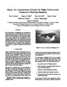
CHAPTER 2. AIRCRAFT FLIGHT DYNAMICS directed North and it is perpendicular to the ZE axis. The YE axis can again be determined using the right-hand rule. • The body reference frame RB is often used when dealing with aircraft. The origin of the reference frame is the center of gravity (COG) of the aircraft. The XB axis lies in the symmetry plane of the aircraft and points forward. The ZB axis also lies in the symmetry plane, but points downward. The YB axis is perpendicular to the XB axis and can again be determined using the right-hand rule. Sometimes we choose the body axes to be aligned with the vehicle principle axes. The origin is generally taken at the aircraft center of gravity or at a fixed reference location relative to the geometry. • The stability reference frame RS is similar to the body-fixed reference frame RB . It is rotated by an angle of attack α about the YB axis. To find this angle α, we must examine the relative wind vector. We can project this vector onto the plane of symmetry of the aircraft. This projection is then the direction of the XS axis. The ZS axis still lies in the plane of symmetry. Also, the YS axis is still equal to the YB axis. So, the relative wind vector lies in the XS YS plane. This reference frame is particularly useful when analyzing flight dynamics. • The aerodynamic or wind reference frame RW is similar to the stability reference frame RS . It is rotated by sideslip angle β about the ZS axis. This is done, such that the XW axis points in the direction of the relative wind vector Va . So the XW axis generally does not lie in the sysmmetry plane anymore. The ZW axis is still equation to the ZS axis. The YW axis can now be found using the right-hand rule. • Finally, there is the vehicle reference frame RV . Contrary to the other systems, this is a left-handed system. Its origin is a fixed point on the aircraft. The XV axis points to the rear of the aircraft. The YV axis points to the left. Finally, the ZV axis can be found using the left-hand rule. (It points upward.) This system is often used by the aircraft manufacturer, to denote the position of parts within the aircraft. 8
2.3. REFERENCE FRAMES
Figure 2.1: Aircraft reference frames
2.3.2
Rotation matrices between frames
Based on what has been described above, we can go from one reference frame to any other reference frame, using at most three Euler angles. An Euler angle can be represented by a transformation matrix T. To see how it works, let us consider a vector x1 in reference frame 1. The matrix T21 now calculates the coordinates of the same vector x2 in reference frame 2, according to: x2 = T21 x1
(2.3.1)
Let us suppose we are only rotating about the X axis. In this case, the transformation matrix T21 is quite simple. In fact, it is: 1 0 0 T21 = 0 cos φx sin φx 0 − sin φx cos φx
(2.3.2)
Similarly, we can rotate about the Y axis and the Z axis. In this case, the transformation matrices are, respectively: cos φy 0 − sin φy T21 = 0 1 0 sin φy 0 cos φy
cos φz
and T21 = − sin φz 0 9
sin φz 0 cos φz 0 0 1
(2.3.3)
CHAPTER 2. AIRCRAFT FLIGHT DYNAMICS Rotation matrices have interesting properties. They only rotate points. They do not deform them. For this reason, the matrix columns are orthogonal and, because the space is not stretched out either, these columns must also have length 1. A transformation matrix is thus orthogonal. This implies that: T T−1 21 = T21 = T12
(2.3.4)
However, to define the transformation matrix which allows the transition between the three body centered reference frames: the body reference frame RB , the stability reference frame RS and the wind reference frame RW represented on the fig.(2.1), we proceed first at the body reference frame RB . If we rotate this frame by an angle of attack α around the YB axis, we find the stability reference frame RS . If we then rotate it by the sideslip angle β around the ZB axis, we get the wind reference frame RW . So we can find that:
XW
cos β sin β 0 cos β sin β 0 cos α 0 − sin α = − sin β cos β 0 X S = − sin β cos β 0 0 1 0 XB 0 0 1 0 0 1 − sin α 0 cos α (2.3.5)
by working things out, it appears that the transformation matrix allowing the transition between the body-fixed reference frame RB and wind reference frame RW is as follows:
TW B
cos β cos α sin β cos β sin α = − sin β cos α cos β − sin β sin α − sin α 0 cos α
(2.3.6)
We can perform a similar transformation between the Earth-fixed reference frame RE and the body-fixed reference frame RB . To do that, we first have to rotate over the yaw angle ψ about the ZB axis. We then rotate over the pitch angle θ about the resulting Y axis. Finally, the new resulting reference frame is then rotated over the roll angle φ around its X axis. It results the configuration shown in fig.(2.2). Then, the transformation matrix 10
2.4. THE EQUATIONS OF MOTION
Figure 2.2: Euler angles configuration TBE is such as:
cos θ cos ψ
cos θ sin ψ
− sin θ
TBE = sin φ sin θ cos ψ − cos φ sin ψ sin φ sin θ sin ψ + cos φ cos ψ sin φ cos θ (2.3.7) cos φ sin θ cos ψ + sin φ sin ψ cos φ sin θ sin ψ − sin φ cos ψ cos φ cos θ When analyzing the flight dynamics, we are concerned both with rotation and translation of this axis set with respect to a fixed inertial reference frame. For all practice purposes, the local Earth-fixed reference frame RE is used.
2.4
The equations of motion
In this section the aircraft dynamics is studied. We present the governing equations linking the variables to be controlled to the control inputs available to us. With respect to several references in literature [Stevens and Lewis, 2003], the presentation is focused on arriving at a mathematical model suitable for control design, consisting of a set of first order nonlinear differential equations. For a deeper insight into the mechanics and aerodynamics 11
CHAPTER 2. AIRCRAFT FLIGHT DYNAMICS behind the model, the reader is referred to the aformentioned references [Etkin and Reid, 1996, McLean, 1990, Nelson, 1998].
2.4.1
Equations of motion in the Earth-fixed reference frame RE
The flight dynamics of an aircraft are described by its equations of motion. First, we will use the assumptions that Earth is flat and fixed, and that the aircraft body is rigid. This yields a six (06) degrees of freedom model. The dynamics can be described by a state space model with twelve (12) states. Before let us define: • PAc = (PN , PE , h)T , the aircraft position expressed in the Earth-fixed reference frame RE . • VI = (u, v, w)T , the inertial speed vector expressed in the body reference frame RB . • Va = (u − wX , v − wY , w − wZ )T , the airspeed vector expressed in the body reference frame. • Φ = (φ, θ, ψ)T , the Euler angles describing the orientation of the aircraft relative to the Earth-fixed reference frame. • Ω = (p, q, r)T , the angular velocity of the aircraft expressed in the body-fixed reference frame. where (wX , wY , wZ ) are the components of the wind vector expressed in the body-fixed frame such as: w W X x wY = TBE Wy wZ Wz
(2.4.1)
The only coupling from PAc to other state variables is through the altitude dependance of the aerodynamic pressure. The equations governing the remaining three state vectors 12
2.4. THE EQUATIONS OF MOTION can be compactly written as: dVI |B + mΩ|BE × VI dt dΩBE MG = IG |B + ΩBE × IG ΩBE dt Φ˙ = E(Φ)Ω|BE
(2.4.2b)
1 sin φ tan θ cos φ tan θ E(Φ) = 0 cos φ − sin φ cos φ 0 tan θ cos θ
(2.4.3)
F =m
where
(2.4.2a)
(2.4.2c)
m is the aircraft mass and IG is the aircraft inertia matrix. The forces and moments equations follow from applying the formalism of Newton and the attitude equation results from the relation between the Earth-fixed and the body-fixed reference frames. F and MG represent respectively the sum of the forces and moments acting on the aircraft at the center of gravity. These forces and moments appear from three major sources: • gravity, • engine thrust, and • aerodynamic efforts. Introducing: F = FG + FE + FA
(2.4.4a)
MG = ME + MA
(2.4.4b)
Forces To establish the aircraft equations of motion, we start by examining forces. Our starting point is Newton0 s second law. However, Newton0 s second law only holds in an inertial reference frame. Luckily, the assumptions we have made earlier imply that the Earth-fixed 13
CHAPTER 2. AIRCRAFT FLIGHT DYNAMICS reference frame RE is inertial. However, RB is not an inertial reference frame. So we will derive the equations of motion with respect to RE . Let0 s examine an aircraft. Newton0 s second law states that: �Z � Z d F = dF = Vp dm dt
(2.4.5)
By integrating over the entire body, it can be shown that the right side of this equation equals
d (mVI ), dt
where VI is the velocity of the center of gravity of the aircraft. If the
aircraft has a constant mass, we can rewrite the above equation into: F =m
dVI = mAG dt
(2.4.6)
But it does imply something very importatnt. The acceleration of the center of gravity of the aircraft does not depend on how the forces are distributed along the aircraft. It only depends on the magnitude and direction of the forces. There is one slight problem. The above equation (2.4.6) is expressed in the Earth reference frame. But we usually work in the body-fixed reference frame RB . So we need to convert it. To do this, we can use the rules related to the relative motion: AG =
dVI dVI |E = |B + ΩBE × VI dt dt
inserting (2.4.7) into the above equation (2.4.6) will give: u˙ + qw − rv dVI F =m |B + mΩBE × VI = m v˙ + ru − pw dt w˙ + pv − qu
(2.4.7)
(2.4.8)
As it is mentioned above, the main forces acting on the aircraft body are gravity, engine thrust and aerodynamic efforts forces. Grvaity only gives a force contribution since it acts at the aircraft center of gravity. The gravitational force, mg, directed along the normal of the Earth plane, is considered constant over the altitude envelope. This yields: −mg sin θ FG = mg sin φ cos θ mg cos φ cos θ 14
(2.4.9)
2.4. THE EQUATIONS OF MOTION The thrust force due to the propulsion system can have components that act along each of the body-fixed reference frame RB . Assuming the engine to be positioned so that the thrust acts parallel to the aircraft body X-axis, yields: F T FE = 0 0
(2.4.10)
The aerodynamic forces and moments, or aerodynamic efforts, result due to the interaction between the aircraft body and the incoming airflow. The size and direction of the aerodynamic efforts are determined by the amount of air diverted by the aircraft in different directions [Etkin and Reid, 1996]. The amount of air diverted by the aircraft is mainly decided by: • the speed and density of the airflow (Va , ρ), • the geometry of the aircraft (δa , δe , δr , S, c, b), • the orientation of the aircraft relative to the airflow (α, β) The aerodynamic efforts also depend on other variables, like the angular rates (p, q, r) ˙ but these effects are not as and the time derivatives of the aerodynamic angles (α, ˙ β), pronounced. This motivates the standard way of modeling aerodynamic forces and moments: ˙ ...) Force = qSCF (δa , δe , δr , δth , α, β, p, q, r, α, ˙ β, ˙ ...) Moment = qSlCM (δa , δe , δr , δth , α, β, p, q, r, α, ˙ β, where δa , δe , δr and δth are respectively aileron, elevator, rudder deflections and throttle setting and q denotes the aerodynamic pressure and it is expressed such as: 1 q = ρ(h)Va2 2
(2.4.12)
and captures the density dependance and most of the speed dependance, S is the aircraft wing surface area and l refers to the length of the lever arm connected to the moment. CF 15
CHAPTER 2. AIRCRAFT FLIGHT DYNAMICS and CM are known as aerodynamic coefficients. These are difficult to model analytically but can be estimated empirically through wind tunnel experiments and actual flight tests. Typically, each coefficient is written as a sum of several components, each capturing the dependance of one or more of the variables above. These components can be represented in several ways. A common approach is to store them in look-up tables and use interpolation to compute intermediate values. In other approaches one tries to fit the data to some parameterized function. In the body-fixed reference frame RB , we have the expressions: F X FA = FY FZ
(2.4.13)
where 1 FX = ρ(h)Va2 SCx 2 1 FY = ρ(h)Va2 SCy 2 1 FZ = ρ(h)Va2 SCz 2
(2.4.14a) (2.4.14b) (2.4.14c)
By combining equations (2.4.9), (2.4.10) and (2.4.13) with the equation of motion for forces (2.4.8), we find that: FX + FT m FY v˙ = pw − ru + g sin φ cos θ + m FZ w˙ = qu − pv + g cos φ cos θ + m
u˙ = rv − qw − g sin θ +
(2.4.15a) (2.4.15b) (2.4.15c)
Moments Before starting to study the moments acting on the aircraft, we first examine angular momentum. The angular momentum of an aircraft BG with respect to the center of gravity is defined as: Z BG =
dBG = r × Vp dm 16
(2.4.16)
2.4. THE EQUATIONS OF MOTION where we integrate over every point P in the aircraft. We can substitute: Vp = VI +
dr |B + ΩBE × r dt
(2.4.17)
if we insert (2.4.17) in equation (2.4.16), we can eventually find that: BG = IG ΩBE
(2.4.18)
As it is indicated before the matrix IG is the aircraft inertia matrix, with respect to the center of gravity. It is defined as follows: R R R Ixx −Ixy −Ixz (ry2 + rz2 )dm − (rx ry )dm − (rx rz )dm R R 2 R 2 IG = −Ixy Iyy −Iyz = − (rx ry )dm (rx + rz )dm − (ry rz )dm R R R 2 2 −Ixz −Iyz Izz − (rx rz )dm − (ry rz )dm (rx + ry )dm (2.4.19) we have assumed that the XZ-plane of the aircraft is a plane of symmetry. For this reason, Ixy = Iyz = 0. The moment acting on the aircraft expressed in the Earth-fixed reference frame supposed inertial, with respect to its center of gravity, is given by: Z Z Z d(Vp dm) MG = dMG = r × dF = r × dt
(2.4.20)
where we integrate over the entire body, we can simplify the above relation to: MG =
dBG |E dt
(2.4.21)
The above relation only holds for inertial reference frames. However, we want to have the above relation in RB . So we rewrite it to: MG =
dBG |B + ΩBE × BG dt
(2.4.22)
and by using (2.4.18), we can continue to rewrite the above equation. We find the equation (2.4.4b) which in matrix-form can be written as: Ixx p˙ + (Izz − Iyy )qr − Ixz (pq + r) ˙ MG = Iyy q˙ + (Ixx − Izz )pr + Ixz (p2 − r2 ) Izz r˙ + (Iyy − Ixx )pq + Ixz (qr − p) ˙ 17
(2.4.23)
CHAPTER 2. AIRCRAFT FLIGHT DYNAMICS Note that we have used the fact that Ixy = Iyz = 0. To define the external moments, we can distinguish two types of moments, acting on the aircraft. There are moments caused by gravity, and moments caused by aerodynamic forces. The moments caused by gravity are zero since the resultant gravitational force acts in the aircraft center of gravity. So we only need to consider the moments caused by aerodynamic forces. We denote those as:
L MA = M N
(2.4.24)
where L, M and N denote respectively, the rolling moment, the pitching moment and yawing moment and they are expressed in the body-fixed reference frame such as: 1 L = ρ(h)Va2 SbCl 2 1 M = ρ(h)Va2 ScCm 2 1 N = ρ(h)Va2 SbCn 2
(2.4.25a) (2.4.25b) (2.4.25c)
with Cl , Cm and Cn represent the aerodynamic moments coefficients. They are expressed such as: rb pb + Clp + Clδa δa + Clδr δr 2Va 2Va αc ˙ qc Cm = Cm0 + Cmα α + Cmα˙ + Cm q + Cmδe δe + Cmδth δth 2Va 2Va pb rb Cn = Cn0 + Cnβ β + Cnr + Cnp + Cnδa δa + Cnδr δr 2Va 2Va Cl = Cl0 + Clβ β + Clr
(2.4.26a) (2.4.26b) (2.4.26c)
In addition, the propulsive forces can also create moments if the thrust does not act through the aircraft center of gravity. We assume the engine to be mounted so that the thrust point lies in the body-axes XZ-plane, offset from the center of gravity by ZT P in the body-axes Z-direction results in:
0
ME = FT ZT P 0 18
(2.4.27)
2.4. THE EQUATIONS OF MOTION By combining equations (2.4.22), (2.4.24) with the equation of motion for moments (2.4.21), we find that: p˙ = (a1 p + a2 r)q + a3 L + a4 N
(2.4.28a)
q˙ = a5 pr − a6 (p2 − r2 ) + a7 (M + FT ZT P )
(2.4.28b)
r˙ = (a8 p − a1 r)q + a4 L + a9 N
(2.4.28c)
Here we have introduced: a1 =
(Ixx − Iyy + Izz )Ixz 2 Ixx Izz − Ixz
a4 =
a7 =
Ixz 2 Ixx Izz − Ixz
1 Iyy
a8 =
a2 =
2 (Iyy − Izz )Izz − Ixz 2 Ixx Izz − Ixz
a5 =
a3 =
Izz − Ixx Iyy
2 Ixx (Ixx − Iyy ) + Ixz 2 Ixx Izz − Ixz
Izz 2 Ixx Izz − Ixz
a6 =
a9 =
Ixz Iyy
Ixx 2 Ixx Izz − Ixz
Translational kinematics Since we have the force and moment equations (2.4.13) and (2.4.24), we only need to find the kinematics relations for the aircraft. First, we examine translational kinematics. This concerns the velocity of the center of gravity of the aircraft with respect to the ground. The velocity of the center of gravity, with respect to the ground, is called the kinematic velocity Vk . It is described in the Earth-fixed reference frame RE by: V N Vk = VE −VZ
(2.4.29)
where VN is the velocity component in the Northward direction, VE is the velocity component in the Eastward direction, and −VZ is the vertical velocity component. Note that the minus sign is present because, in the Earth-fixed reference frame, VZ is defined to be positive downward. However, in the body-fixed reference frame RB , the inertial speed 19
CHAPTER 2. AIRCRAFT FLIGHT DYNAMICS vector of the center of gravity, with respect to the ground, is given by: u VI = v w
(2.4.30)
To relate those two vectors to each other, we need the transformation matrix TBE defined in (2.3.7). This gives us: Vk = TEB VI = TTBE VI
(2.4.31)
This is the translational kinematic relation. We can use it to derive the change of the aircraft position. To do that, we simply have to integrate the velocities. Thus, we have: Z t Z t Z t VZ dt (2.4.32) VE dt and z(t) = − VN dt, y(t) = x(t) = 0
0
0
where: cos θ cos ψ sin φ sin θ cos ψ − cos φ sin ψ cos φ sin θ cos ψ + sin φ sin ψ u x˙ y˙ = sin ψ cos θ sin φ sin θ sin ψ + cos φ cos ψ cos φ sin θ sin ψ − sin φ cos ψ v − sin θ sin φ cos θ cos φ cos θ w z˙ (2.4.33) Rotational kinematics This concerns the motion of rotation of the aircraft. In the Earth-fixed reference frame RE , ˙ θ˙ and ψ. ˙ However, in the body-fixed the rotational velocity is described by the variables φ, frame, the rotational velocity is described by roll, pitch and yaw rates (p, q, r), respectively. The relation between these two set of variables can be shown from the equation (2.4.2c) as follows: φ˙ = p + tan θ(q sin φ + r cos φ)
(2.4.34a)
θ˙ = q cos φ − r sin φ
(2.4.34b)
ψ˙ =
1 (q sin φ + r cos φ) cos θ 20
(2.4.34c)
2.4. THE EQUATIONS OF MOTION and inversely: p 1 0 − sin θ φ˙ q = 0 cos φ sin φ cos θ θ˙ r 0 − sin φ cos φ cos θ ψ˙
(2.4.35)
Summary The state equations which describe the aircraft translational and rotational motions expressed in the Earth-fixed reference frame are gathered such as: 1. State equations describing aircraft angular velocities: p˙ = (a1 p + a2 r)q + a3 L + a4 N
(2.4.36a)
q˙ = a5 pr − a6 (p2 − r2 ) + a7 (M + FT ZT P )
(2.4.36b)
r˙ = (a8 p − a1 r)q + a4 L + a9 N
(2.4.36c)
2. State equations describing aircraft Euler angles: φ˙ = p + tan θ(q sin φ + r cos φ)
(2.4.37a)
θ˙ = q cos φ − r sin φ
(2.4.37b)
ψ˙ =
1 (q sin φ + r cos φ) cos θ
(2.4.37c)
3. State equations describing airspeed components: FX + FT m FY v˙ = pw − ru + g sin φ cos θ + m FZ w˙ = qu − pv + g cos φ cos θ + m
u˙ = rv − qw − g sin θ +
(2.4.38a) (2.4.38b) (2.4.38c)
4. State equations describing aircraft position: x˙ cos θ cos ψ sin φ sin θ cos ψ − cos φ sin ψ cos φ sin θ cos ψ + sin φ sin ψ u y˙ = sin ψ cos θ sin φ sin θ sin ψ + cos φ cos ψ cos φ sin θ sin ψ − sin φ cos ψ v z˙ − sin θ sin φ cos θ cos φ cos θ w (2.4.39) 21
CHAPTER 2. AIRCRAFT FLIGHT DYNAMICS
2.4.2
Equations of motion in the wind reference frame RW
The aerodynamic forces are also commonly expressed in the wind reference frame RW related to the body reference frame RB as indicated in fig.(2.1), where we have: −D FA |W = Y (2.4.40) −L with L, Y and D denote respectively lift, side and drag forces. They are expressed as follows: 1 L = ρ(h)Va2 SCL 2 1 Y = ρ(h)Va2 SCY 2 1 D = ρ(h)Va2 SCD 2
(2.4.41a) (2.4.41b) (2.4.41c)
where the lift, side and drag aerodynamic forces coefficients, CL , CY and CD mainly depend on the angle of attack α and sideslip angle β, respectively. Their analytical expressions depend on control objectives and they are generally presented [Etkin and Reid, 1996,Etkin, 1985, McLean, 1990] such as: q + CLδe δe Va pb rb + C Yp + C Yδ r δ r + C Yβ β + C Yr 2Va 2Va
CL = CL0 + CLα α + CLq C Y = C Y0
CD = CD0 + CDα α + CDα2 α2
(2.4.42a) (2.4.42b) (2.4.42c)
Note that, the aerodynamic forces FX , FY and FZ can be expressed in the wind reference frame RW such as: FX = −D cos α cos β − Y sin β cos α + L sin α
(2.4.43a)
FY = −D sin β + Y cos β
(2.4.43b)
FZ = −D sin α cos β − Y sin α sin β − L cos α
(2.4.43c)
22
2.4. THE EQUATIONS OF MOTION We can rewrite the force equations in terms of angle of attack α, sideslip angle β and airspeed Va variables by performing the following change of variables:
u = Va cos α cos β + wX
(2.4.44a)
v = Va sin β + wY
(2.4.44b)
w = Va sin α cos β + wZ
(2.4.44c)
as a first result, we can get:
Va =
p
(u − wX )2 + (v − wY )2 + (w − wZ )2 � � w − wZ α = arctan u − wX � � v − wY β = arcsin Va
(2.4.45a) (2.4.45b) (2.4.45c)
Then, the equations of drag, lift and side forces expressed in the wind reference frame RW become:
D = −FX cos α cos β − FY sin β − FZ sin α cos β
(2.4.46a)
L = FX sin α − FZ cos α
(2.4.46b)
Y = −FX cos α sin β + FY cos β − FZ sin α sin β
(2.4.46c)
where the state equations describing airspeed Va , angle of attack α and sideslip angle β 23
CHAPTER 2. AIRCRAFT FLIGHT DYNAMICS behaviors are respectively such as: 1 V˙ a = (−D + FT cos α cos β + mg1 ) + p(wY sin α cos β + wZ sin β) m + q cos β(wZ cos α + wX sin α) + r(wX sin β + wY cos α cos β)
(2.4.47a)
− w˙ X cos α cos β − w˙ Y sin β − w˙ Z sin α cos β 1 α˙ = q − (p cos α + r sin α) tan β + (−L − FT sin α + mg2 ) mVa cos β � � 1 + q(wZ sin α + wX cos α) − wY (p cos α + r sin α) + w˙ X sin α − w˙ Z cos α Va cos β (2.4.47b) �
1 1 (Y − FT cos α sin β + mg3 ) + −wX (q sin α sin β + r cos β) β˙ = p sin α − r cos α + mVa Va + wY sin β(p sin α − r cos α) + wZ (q cos α sin β + p cos β) + w˙ X cos α sin β � − w˙ Y cos β + w˙ Z sin α sin β (2.4.47c) with the contributions g1 , g2 and g3 due to the gravity are given by: g1 = g(− cos α cos β sin θ + sin β cos θ sin φ + sin α cos β cos θ cos φ) g2 = g(cos α cos θ cos φ + sin α sin θ) g3 = g(cos β cos θ sin φ + cos α sin β sin θ − sin α sin β cos θ cos φ)
(2.4.48a) (2.4.48b) (2.4.48c)
In no wind condition, airspeed, angle of attack and sideslip angle equations are: 1 V˙ a = (−D + FT cos α cos β + mg1 ) m 1 α˙ = q − (p cos α + r sin α) tan β + (−L − FT sin α + mg2 ) mVa cos β 1 (Y − FT cos α sin β + mg3 ) β˙ = p sin α − r cos α + mVa
(2.4.49a) (2.4.49b) (2.4.49c)
For flight path angles, the mathematical expressions are derived as follows: ~ V~I = V~a + W 24
(2.4.50)
2.4. THE EQUATIONS OF MOTION ~ are respectively the inertial, the airspeed and the wind speed vectors. where V~I , V~a and W The components of the inertial airspeed vector expressed in the Earth frame are such as: V cos γI cos µ I ~ VI = VI cos γI sin µ (2.4.51) −VI sin γI
→
− where VI = VI , γI is the inertial path angle and µ is the horizontal orientation of the inertial speed. The airspeed vector is given in the body frame in terms of angle of attack and sideslip angle by: V~a =
Va cos α cos β Va sin β Va sin α cos β
(2.4.52)
As it is shown in (2.3.7), the rotation matrix TEB = TTBE allows the transition from the body frame to the local Earth frame. Then we have: V cos µ cos γI V cos α cos β W I a x VI sin µ cos γI = TEB (φ, θ, ψ) Va sin β + Wy −VI sin γI Va sin α cos β Wz
(2.4.53)
it results: s� VI = Va
Wx u1 + Va
�2
�
Wy + u2 + Va
�2
�
Wz + u3 + Va
�2 (2.4.54)
with: u1 = Cθ Cψ Cα Cβ + (Sφ Sθ Cψ − Cφ Sψ )Sβ + (Cφ Sθ Cψ + Sφ Sψ )Sα Cβ
(2.4.55a)
u2 = Sψ Cθ Cα Cβ + (Sφ Sθ Sψ + Cφ Cψ )Sβ + (Cφ Sθ Sψ − Sφ Cψ )Sα Cβ
(2.4.55b)
u3 = −Sθ Cα Cβ + Sφ Cθ Sβ + Cφ Cθ Sα Cβ
(2.4.55c)
v
− u →
W
2 u ~ W
t ~ VI = Va 1 + 2U +
Va Va
(2.4.56)
or:
25
CHAPTER 2. AIRCRAFT FLIGHT DYNAMICS with:
u 1 ~ = U u 2 u3
(2.4.57)
Since from (2.4.56) we can write:
−
− 2
→
→ 2
− 2 → ~ ~
VI = Va + 2Va .W + W Then: p VI = Va 1 + η
with
(2.4.58)
− →
W
2 ~ 2V~a .W
η= +
Va Va2
(2.4.59)
~ is the unity vector along the airspeed direction: and it appears that U ~ ~ = Va U Va
(2.4.60)
The inertial and air path angles are then given respectively by: � � Va Wz γI = − arcsin (− sin θ cos α cos β + sin φ cos θ sin β + cos φ cos θ sin α cos β) + VI VI (2.4.61a) � γa = − arcsin
Va (− sin θ cos α cos β + sin φ cos θ sin β + cos φ cos θ sin α cos β) VI
� (2.4.61b)
~ = ~0, φ = 0 and β = 0, we get the classical formula: Observe that when W γI = γa = θ − α
(2.4.62)
and that when φ = 0 and β = 0: �
Wz Va γI = − arcsin − sin γa + VI VI
2.5
� (2.4.63)
Partial flight dynamics equations
In the literature [Stengel, 2004, McLean, 1990, Nelson, 1998], several reasons are advanced for the separate study of longitudinal and lateral dynamics of an aircraft. The most significant ones are described below: 26
2.5. PARTIAL FLIGHT DYNAMICS EQUATIONS • Flight plans generated by a Flight Management System (FMS) are composed of a vertical and horizontal components leading to the realization of either longitudinal or lateral maneouvers according to the phase of the flight. • When an aircraft is either in steady, level flight or climbing or descending in the vertical plane, longitudinal and lateral-directional variations are uncoupled to first order, • Reducing the difficulty level by limiting the number of nonlinear differential equations to those which characterize either the longitudinal dynamic effects, or the lateral dynamic effects.
2.5.1
Longitudinal equations of motion
For flight in the vertical plane, the longitudinal equations of motion describe changes in axial and normal velocity u and w, pitch rate and angle q and θ, range x, and altitude z. The six nonlinear differential equations are derived from the subsection above such as: FX + FT m FZ w˙ = qu + g cos θ + m
u˙ = −qw − g sin θ +
(2.5.1a) (2.5.1b)
x˙ = u cos θ + w sin θ
(2.5.1c)
z˙ = −u sin θ + w cos θ
(2.5.1d)
θ˙ = q
(2.5.1e)
q˙ =
1 (M + FT ZT P ) Iyy
(2.5.1f)
It is possible to rewrite the longitudinal equations of motion in terms of angle of attack α, flight path angle γ and airspeed Va variables by proceeding to the change of variables reported in (2.4.44a) to (2.4.44c) and also by: α=θ−γ 27
(2.5.2)
CHAPTER 2. AIRCRAFT FLIGHT DYNAMICS This gives us the longitudinal equations of motion expressed in the wind reference frame RW as follows:
x˙ = Va cos γ + wX cos θ + wZ sin θ
(2.5.3a)
z˙ = −Va sin γ − wX sin θ + wZ cos θ
(2.5.3b)
1 V˙ a = (−D + FT cos α − mg sin γ) + q(wZ cos α − wX sin α) + w˙ X cos α + w˙ Z sin α m (2.5.3c) � � 1 1 (−L − FT sin α + mg cos γ) + q(wZ sin α − wX cos α) + w˙ Z cos α − w˙ X sin α α˙ = q + mVa Va (2.5.3d) � 1 1 γ˙ = (FT sin α + L − mg cos γ) − q(wZ sin α − wX cos α) + w˙ Z cos α − w˙ X sin α mVa Va �
(2.5.3e) θ˙ = q q˙ =
1 (M + FT ZT P ) Iyy
(2.5.3f) (2.5.3g)
with D and L are respectively given as follows:
D = −FX cos α − FZ sin α
(2.5.4a)
L = FX sin α − FZ cos α
(2.5.4b)
Aircraft longitudinal equations of motion expressed in the aerodynamic (wind) reference 28
2.5. PARTIAL FLIGHT DYNAMICS EQUATIONS frame RW when the wind components wX , wZ are considered null, are: x˙ = Va cos γ
(2.5.5a)
z˙ = −Va sin γ
(2.5.5b)
1 V˙ a = (−D + FT cos α − mg sin γ) m 1 γ˙ = (FT sin α + L − mg cos γ) mVa θ˙ = q q˙ = α˙ = q +
2.5.2
1 (M + FT ZT P ) Iyy
1 (−L − FT sin α + mg cos γ) mVa
(2.5.5c) (2.5.5d) (2.5.5e) (2.5.5f) (2.5.5g)
Lateral equations of motion
The lateral-directional equations of motion describe changes in lateral velocity v and roll and yaw rates p and r in the body-fixed reference frame. The roll and yaw angles φ and ψ orient the body-fixed reference frame axes with respect to the inertial frame, and the translational position is expressed by the cross range y. The six nonlinear differential equations are as follows: y˙ = u sin ψ + v cos φ cos ψ − w sin φ cos ψ
(2.5.6a)
p˙ = a3 L + a4 N
(2.5.6b)
r˙ = a4 L + a9 N
(2.5.6c)
v˙ = pw − ru + g sin φ +
FY m
(2.5.6d)
φ˙ = p
(2.5.6e)
ψ˙ = r cos φ
(2.5.6f)
note that, the above equations are derived based on the following assumption: θ = q = 0. It is possible to rewrite the sideslip angle β dynamics from equations (2.4.45c) and 29
CHAPTER 2. AIRCRAFT FLIGHT DYNAMICS (2.4.45a) such as: � � 1 ˙ β = p sin α − r cos α + Y − FT cos α sin β + mg(sin φ cos β − sin α sin β cos φ) mVa � � 1 + wY sin β(r cos α − p sin α) + w˙ Y cos β Va (2.5.7) with: D = −FX cos α cos β − FY sin β − FZ sin α cos β L = FX sin α − FZ cos α Y = −FX cos α sin β + FY cos β − FZ sin α sin β If the side wind component wY is neglected, the aircraft lateral flight dynamics expressed in the aerodynamic reference frame in term of the sideslip equation is now such as:
� � 1 ˙ β = p sin α − r cos α + Y − FT cos α sin β + mg(sin φ cos β − sin α sin β cos φ) (2.5.9) mVa
2.6
Conclusion
The flight dynamics of an aircraft are modelized in general by complex nonlinear coupled differential equations where the aerodynamic effects are complicating factors. The motion of a flying aircraft is composed of a rotation and a translation where the former is considered to be a fast motion while the later is taken as a slower motion. In fact even if the flight equations appear as a very complex bundle of formulas, a detailed analysis makes appear a particular structure composed of the decoupling between longitudinal and lateral motion and of a causal relationship between fast and slow dynamic modes. This particular structure has been exploited very early to design the first autopilot/autoguidance systems.
30
Chapter 3 Classical Flight Control Law Design 3.1
Introduction
In this chapter, we introduce the main classical approaches which have been developed for the design of control laws for autopilots and autoguidance systems devoted to transport aircraft. After introducing the principles on which the earlier successful design approaches where based, more recent multi-dimensional flight control law design techniques are presented. Then the way the Flight Management System (FMS) generates guidance directives is discussed while current flight control modes encountered in a modern transportation aircraft are described. Finally in the conclusion some of the main limitations of current flight control law design approaches are pointed out.
3.2
Classical approach to flight control law synthesis
We describe here an early approach that has been adopted by major design offices to develop the first control laws for automatic piloting and guiding of transport aircraft. The approach developed in the area of analog computers (late fifties) has largely been 31
CHAPTER 3. CLASSICAL FLIGHT CONTROL LAW DESIGN reused for autopilots using digital computers (from early seventies). Since then, advances in Automatic Control theory and technology of digital computers (computational speed, storage capacity, reliability, weight and size) were used to develop control laws much more efficient and acceptable by pilots (decoupled control, automatic normal load factor holding, for example). The development of control laws for such a nonlinear multidimensional system, the aircraft, posed at that time a challenge to Automation. The adoption of three principles allowed the decomposition of this problem into sub problems accessible to the basic control theory available at the time: the single input-single output continuous linear control theory. Thus the basic functions for auto control and guidance could be achieved in a practical way, resulting in acceptable performances.
3.2.1
Basic principles adopted for flight control law synthesis
The longitudinal/lateral separation of small movements of the aircraft around an equilibrium state It was considered that the autopilot had to make the aircraft evolve in a progressive way from a static equilibrium to another. It appears that in these conditions, longitudinal and lateral motion of the aircraft present second order small couplings. Thus the first principle used in the design of automatic flight control laws has been to consider separately the small movements of the plane around an equilibrium position in its longitudinal plane and in its lateral plane. This led to consider separately the autopilot modes to master the movement of the aircraft in the vertical and lateral planes.
Decoupling of control channels It seemed interesting, to ease the operation of the whole autopilot system, to assign, from the point of view of the pilot, the automatic control channels to different decoupled tasks. A current assignment of the control channels is such: 32
3.2. CLASSICAL APPROACH TO FLIGHT CONTROL LAW SYNTHESIS
Table 3.1: Assignment of control channels to piloting/guidance modes Longitudinal mode
Longitudinal attitude control (autopilot acting on the longitudinal elevator).
Longitudinal mode
Speed control (Auto-throttle or computing of thrust acting on the engine).
Lateral mode
Lateral attitude control (lateral autopilot acting on the ailerons)
Lateral mode
Yaw control (Lateral stabilizer acting on the rudder)
The application of this principle makes it possible to clearly organize the interface between the pilot and the autopilot systems. In fact, there are significant couplings between longitudinal and lateral movements of the aircraft (for example highlighted during a banked turn), between longitudinal modes (holding glide and reduced speed holding at approach) and between lateral modes (steady turn). Thus, the control laws developed by various calculators autopilot should take into consideration these coupling by adding correction terms, or by the introduction of limitations to ensure the working of assumptions (limitations to small movements). The superposition principle of control loops One of the main limitations of servo control theory was to apply only to SISO (single input-single output) systems and thus to dispose of a unique control input to control (hold value or change of value), of a single output. Yet, even after application of the first two principles, the systems to be controlled remained of the SIMO (single input multi-output) class. For example in the case of the longitudinal (pitch) channel for the elevator deflection δe as input, there are numerous output candidates: pitch rate q, pitch angle θ, angle of attack α, path angle γ, vertical speed Vz and altitude z This limitation of the theory has been bypassed by ranking the output signals according 33
CHAPTER 3. CLASSICAL FLIGHT CONTROL LAW DESIGN
Figure 3.1: Frequency decoupling and causality to their rate of change and taking into account causal relationships between them. Thus, the servo control of the fastest dynamics modes will provide to the needs of the servo control of the slower dynamics modes. This is the principle of superposition of servo control loops, which in practice must obey to Naslin’s frequency decoupling condition [Naslin, 1965]. Then to the serial system given below: (where S1 is a fast signal influencing signal S2 which evolves more slowly and which in its turn influences the output signal S3 whose evolution is even slower and whose value is to be set to a reference value S3c ), can be associated a control system composed of three superposed control loops to which corresponds a cascaded control law such as: u = K1 (S1c − S1m )
(3.2.1)
with: S1c = K2 (S2c − S2m ) and S2c = K3 (S3c − S3m ) where K1 , K2 and K3 are direct control channel gains and where the m index corresponds to a measured signal. It is always possible to improve the control system by adding corrections such as derivative action (improving the stability of the controlled system), integral action (improving the accuracy of the controlled system) and by limiting in position or rate the variation of internal set points (here S2c and S1c ) and setting the gain values K1 , K2 and K3 according to the current position in the flight domain. 34
3.2. CLASSICAL APPROACH TO FLIGHT CONTROL LAW SYNTHESIS The principle of superposition of control loops when applied to flight control then leads to the organization of the autopilot in two main loops: • The small loop which controls the attitude angles of the aircraft (angles φ and θ) or the load factor nz and the roll rate p and which is therefore associated with the auto piloting functions. • The large loop which controls the aircraft guidance parameters and which is therefore associated with the auto guidance functions. To these two loops can be added an inner loop corresponding to the physical actuator (in general a hydraulic device) closed loop servo control.
3.2.2
Examples of implementation of the basic design principles
Here is schematically displayed the implementation of the traditional approach to the design of the main guidance modes present in the first generation of autopilots and based on PID technique: altitude hold, speed control and heading acquisition and hold. For the longitudinal channel with altitude hold at Zc : Z δe =
Kθ (θc − θ)dt − Kq q
with θc = KZ (Zc − Z) − KVZ VZ
(3.2.2)
For the thrust channel in speed hold mode the fuel flow variation is given by: Z Q = KP N (N1c − N1 ) + KIN
(N1c − N1 )dt + KDN (N1c − N1 ) with N1c = KV (Vc − V ) (3.2.3)
where N1 is the rotation speed of the fan, Q is the fuel flow, V is the airspeed and Vc is the desired airspeed (often computed from a desired Mach number). For the roll channel in heading mode, the aileron deflection can be given by: Z δa = KP φ (φc − φ) +
KIφ (φc − φ)dt + KDφ p 35
(3.2.4)
CHAPTER 3. CLASSICAL FLIGHT CONTROL LAW DESIGN with limitation rules such as: φc = 35◦
if Kψ (ψc − ψ) ≥ 35◦
φc = Kψ (ψc − ψ) if φc = −35◦
3.3
− 35◦ ≤ Kψ (ψc − ψ) ≤ 35◦
(3.2.5)
if Kψ (ψc − ψ) ≤ 35◦
Recent approaches for longitudinal control law synthesis
In this section we present the main methods developed more recently for the synthesis of longitudinal and lateral control laws and characterized by a multi input-multi output (MIMO) approach. Many of these methods can in fact be applied globally (longitudinal and lateral movements) to the dynamic control of the plane, but for the sake of clarity, we will first deal only with the longitudinal control problem. For this we first introduce an analytical model reference nonlinear dynamics before reviewing the different synthesis techniques and elements that can be added to the relevant laws to make them more robust to model uncertainties used and deal with external disturbances acting on the longitudinal flight dynamics.
3.3.1
Modal control
This technique has been developed in the late of heighties. In this case, the control objectives are to make the output signals reach their preset reference values while dynamic behavior is turned acceptable with respect to different criteria (stability, response time, damping, etc.). The general form of the control law is such as [Porter and Crossley, 1972, Gawronski, 1998, Stirling, 2001]: u(t) = −Gx(t) + Hy c
with x(t) ∈ Rn ,
y c ∈ Rp
and u(t) ∈ Rm
(3.3.1)
where the term −Gx(t) is called the state feedback and the term Hyc is said direct term. The control law is then completely defined by the choice of gains matrices G and H. The 36
3.3. RECENT APPROACHES FOR LONGITUDINAL CONTROL LAW SYNTHESIS gain G will allow to choose the modal dynamics (eigenvalues and eigenvectors possibly) of the closed-loop controlled system while the choice of H will insure accuracy in the acquisition of outputs reference values. In the case where the values for the outputs change over time, if the modal dynamic closed-loop system is much faster than output signals, it will be possible to follow effectively their progress. Modal control can also meet the important objectives of decoupling between inputs, outputs and acquired dynamic modes. The controlled linear system follows then the general state equation: x˙ = (A − BG)x + BHy c + Ew
(3.3.2)
y = Cx where w is a vector representing external inputs such as perturbations. Considering the eigenvalues (λ1 , λ2 , ..., λn ) of (A − BG), the corresponding right eigenvectors (V 1 , V 2 , ..., V n ) and left eigenvectors (U 1 , U 2 , ..., U n ), we get the following modal representation for the controlled system: ˙ = AX + U BHyc + U Ew X
(3.3.3a)
x = V X, y = CV X, u = −GV X + Hy c UT 1 . U = . and V = [V 1 , V 2 , ..., V n ] . U Tn
(3.3.3b)
(3.3.3c)
So we get the structural representation of these controlled dynamics as shown in fig.(3.2). It is clear in this diagram that matrix U distributes inputs on the dynamic modes, matrix V distributes the dynamic modes on the state, the outputs and the closed-loop term of the control law. The decoupling constraints can be expressed as algebraic orthogonality conditions involving either the right eigenvectors or the left eigenvectors of (A − BG): • Entry reference value yjc does not activate mode Xi if: U Ti BHf uj = 0 37
(3.3.4)
CHAPTER 3. CLASSICAL FLIGHT CONTROL LAW DESIGN
Figure 3.2: Structural representation of controlled system where f uj is the j th column vector of the identity matrix of order m , Im . • Mode Xi does not activate the xj state component if: (f xj )T V i = 0
(3.3.5)
where f xj is the j th column vector of the identity matrix of order n, In . • Mode Xi does not activate the output component yj if: (f yj )T CV i = 0
(3.3.6)
where f yj is the j th column vector of the identity matrix of order p, Ip . The calculation of G, once the eigenvalues λi , i = 1 to n, of the controlled system are fixed can be reduced to searching vectors from the kernels of the endomorphisms represented by the matrix operators [A − λi In , B], i = 1 to n, which should satisfy some additional constraints related with other control objectives. Writting these vectors [V i
W i ]T , where: W i = −GV i ,
i = 1, ..., n
(3.3.7)
the state feedback gain G is given by the expression: G = −[W 1 , ..., W i , ..., W n ][V 1 , ..., V i , ..., V n ]−1 = −W U 38
(3.3.8)
3.3. RECENT APPROACHES FOR LONGITUDINAL CONTROL LAW SYNTHESIS
Figure 3.3: Example of input output decoupling four order system
Regarding the choice of the feed forward gain H, once gain G has been chosen, it should lead the static component of the output to be equal to the assigned reference value y c . This will be always possible when the controlled system is governable. Then we get: � �−1 −1 H = − C[A − BG] B
(3.3.9)
In fact, the choice of too ambitious objectives such as the complete remodeling of the dynamics of the system, to make it able to follow dynamic output trajectories as well as to meet decoupling constraints, will sometimes lead to speed and position demands for the actuators incompatible with their real performance. The linear quadratic regulator (LQR) control approach provides a rather simple way to tackle with the efforts demanded to the actuators while providing a state linear feedback control solution [Wolovich, 1995, Isidori and Hollot, 1995].
3.3.2
A reference model for longitudinal flight dynamics
Starting from the general expressions of Flight Mechanics [Etkin and Reid, 1996, Nelson, 1998], assuming no wind and perfect (no time delay, no error) actuators and sensors 39
CHAPTER 3. CLASSICAL FLIGHT CONTROL LAW DESIGN dynamics, it is possible to retain the following model for longitudinal flight dynamics: 1 V˙ = [−D + T cos α − mg sin γ] m 1 γ˙ = [L + T sin α − mg cos γ] mV M q˙ = Iy
(3.3.10)
z˙ = −V sin γ With the complementary relationships: θ =α+γ θ˙ = q
(3.3.11)
Here D is the aerodynamic drag force, L is the aerodynamic lift force, M is the pitching moment, the engine thrust is T , V is the airspeed, γ is the flight path angle, α is the angle of attack, q denotes the pitch rate, z is the flight level and g the acceleration of gravity. We assume that we dispose of analytical expressions for the lift, the drag and the pitching moment. Then we have in general the parametrized expressions: 1 D = ρV 2 S(CD0 + CDδe δe + CDF δF ) 2 1 L = ρV 2 S(CL0 + CLδe δe + CLF δF ) 2 1 2 qc M = ρV Sc(Cm0 + Cmground + Cmq + Cmδe δe + CmF δF ) 2 2V
(3.3.12a) (3.3.12b) (3.3.12c)
where δe and δF represent the elevator and flaps deflections, respectively. ρ is the air density (kg/m3 ), S denotes an aerodynamic reference surface area, l denotes the reference chord, and the Ci are aerodynamic parameters which depend mainly on the value of the angle of attack and the Mach number.
3.3.3
Classical linear approach for flight control law synthesis
We consider here the case where neglecting the dynamics of the elevator, we assume that the position of the flaps is neutral and that the engine dynamics are well represented by a first order system with time constant τT . 40
3.3. RECENT APPROACHES FOR LONGITUDINAL CONTROL LAW SYNTHESIS Table 3.2: Example of values for the aerodynamic derivatives of a wide body aircraft Parameter
Value
Parameter
Value
Parameter
Value
Xu
-0.0218 s−1
Zu
-0.0569 s−1
Mα
-1.6165 s−2
Xα
0.373 m/s2
Zα
-103.328 m/s
MT
0 s−2
XT
-0.0604 s−1
ZT
0 s−1
Mδe
-1.2124 s−2
Xδe
0 m/s2
Zδe
-5.590 m/s2
Mu
-0.000328 m−1 .s−1
τT
2s
-
-
Mq
-0.4038 s−1
The linearization of the longitudinal dynamics around an equilibrium situation then leads to relations between the small variations of the different longitudinal flight variables and their rates of change:
∆V˙ = Xu ∆V + Xα ∆α − g∆θ + XT ∆T + Xδe ∆δe ∆α˙ = Zu ∆V + Zα ∆α + ∆q + ZT ∆T + Zδe ∆δe ∆q˙ = Mu ∆V + Mα ∆α + Mq ∆q + MT ∆T + Mδe ∆δe
(3.3.13)
∆θ˙ = ∆q 1 1 ∆T˙ = − ∆T + ∆Tc τT τT
Where the coefficients Xu , Xα , XT , Xδe , Zu , Zα , ZT , Zδe , Mu , Mα , Mδe , MT and Mq are computed at the equilibrium situation. In general the values of these coefficients vary slightly from one equilibrium point to another within some limited range of speed and altitude. For example, considering a B747-200 in cruise at z = 12192m (FL400) with an airspeed of 265.4m/s (M = 0.9) [Roskam, 2003], we have the following values for the aerodynamic derivative coefficients: 41
CHAPTER 3. CLASSICAL FLIGHT CONTROL LAW DESIGN Then, we obtain the following state space representation:
∆V˙
X Xα 0 −g XT ∆V 0 X δe u ∆α˙ Zu Zα 1 0 ZT ∆α 0 Zδe ∆T c ∆q˙ = Mu Mα Mq 0 MT ∆q + 0 Mδe ∆δ e ˙ ∆θ 0 0 1 0 0 ∆θ 0 0 ∆T˙ 0 0 0 0 −1/τT ∆T 1/τT 0
(3.3.14)
In general the numerical values of the coefficients are such that the model is asymptotically stable and globally controllable. Similarly, in general it will be globally observable from the measurement of outputs ∆V and θ. As basic control objective (autopilot) it can be assumed that the pitch angle should vary from an initial value θ0 to a reference value θc , while the speed of the aircraft remains at its initial value V0 . A whole variety of techniques for synthesizing control laws is then available in the literature [Magni et al., 1997] to meet these objectives: from frequency decoupling and superposition of control loops, to linear quadratic control, modal control (see previous section), nonlinear dynamic inversion, etc. In general, the resulting law will be composed of a linear state or output feedback and a feed-forward term with the independent inputs:
∆Tc ∆δe
= −
GT V
GT α GT q GT θ
GpV
Gpα
Gpq
Gpθ
∆V ∆α GT T HT θ ∆θc ∆q + H GpT pθ ∆θ ∆T
(3.3.15)
In this expression, some terms may be neglected in order to simplify the control law without a noticeable degradation of performance. Moreover, as a measure of ∆T is in general not available, it will be necessary to construct a state observer to replace ∆T by an estimate. Other problems resulting from different accuracy levels in the measurement of different flight variables, may appear when implementing the state feedback control law, needing the introduction of some kind of filtering. Also, some integral terms will be added 42
3.4. FLIGHT MANAGEMENT GENERATION OF GUIDANCE DIRECTIVES to the control law to compensate for model errors and the non consideration of second order lateral effects over the longitudinal flight dynamics.
3.4
Flight management generation of guidance directives
Today auto guidance modes can be either selected by the pilot through the flight control unit interfacing him with the auto flight computer or chosen automatically by the Flight Management System (FMS) of the aircraft. • In normal situation this action will be necessary to make the aircraft follow the flight plan constructed by its corresponding flight plan generation function. Many time, the vertical profile to be followed is quite complex and needs frequent mode changes with inclusion of pertinent reference values while lateral guidance may integrate complex maneuvers, then the Flight Management System has become an essential tool for the efficiency of flight. • In critical situation, either the pilot or an auto flight protection will impose new guidance directives to get rid of the hazardous situation.
3.4.1
FMS lateral guidance
The lateral guidance function of the Flight Management System, the L-NAV function, computes dynamic guidance data based on the predicted lateral profile performed by its trajectory prediction module to make the aircraft follow the lateral flight plan composed of a succession of straight and curved legs. The data are composed of the classic horizontal situation information (distance to go to the active lateral waypoint, desired track (DT RK), track angle error (T RKERR ), cross-track error (XT RK), drift angle (DA), bearing to the go to waypoint (BRG) and lateral track change alert-LNAV alert). A common approach to compute this data is to convert the lateral path lateral/longitudinal point represen43
CHAPTER 3. CLASSICAL FLIGHT CONTROL LAW DESIGN tation and aircraft current position to Earth-referenced unit vectors using the following relationships: X = cos (lat) cos (lon) Y = cos (lat) sin (lon)
(3.4.1)
Z = sin (lat) where (lat) and (lon) represent the latitude and longitude aircraft points, respectively. This approach can also be used to compute the distance and course information between points that are displayed to the crew for the flight plan presentation. The lateral function also supplies data for a graphical representation of the lateral path to the navigation display, if the aircraft is so equipped, such that the entire lateral path can be displayed in an aircraftreferenced format or a selected waypoint referenced format. The data for this display are in general formatted as latitude/longitude points with identifiers and latitude/longitude points with straight and curved vector data connecting the points. Already, FMS are able to produce a bit map image of the lateral path to transmit to the navigation display. Lateral leg switching and waypoint sequencing The lateral path is composed of several segments and most lateral course changes are performed as flyby transitions. Therefore anticipation of the activation of the next vertical leg is required, such that a smooth capture of that segment is performed without path overshoot. The turn initiation criteria are based on the extent of the course change, the planned bank angle for the turn manoeuver, and the ground speed of the aircraft, according to variations of the basic formula: Turn Radius =
VG2 g tan φn
(3.4.2)
where VG is the ground speed and φn is the nominal bank angle during a balanced turn maneuver. The roll in distance before the initiation of the turn is selected based on how quickly the aircraft responds to a change in the aileron position. Turn initiation and waypoint sequence follow the same algorithms except the course change is reduced from 44
3.4. FLIGHT MANAGEMENT GENERATION OF GUIDANCE DIRECTIVES the actual course change to delay the leg transition. The amount of course change reduction is determined by a balance in the airspace utilized to perform the overall manoeuver. For flyover transitions, the activation of the next leg occurs at the time a flyover waypoint is sequenced.
Bank control Based on the aircraft current position provided by the navigation function of the FMS and the stored lateral profile provided by the trajectory prediction function of the FMS, lateral guidance may generate a bank reference value for the flight control system. This command is both magnitude and rate limited based on aircraft limitations, passenger comfort, and airspace considerations. The bank command is generated in accordance with the straight and curved path segments that compose the lateral profile. The bank control is in general a simple control law driven by the lateral cross-track error and the track error as given here: φc = KXT RK .XT RK + KT RK .T RKERR + φn
(3.4.3)
where φn is the nominal planned bank angle and where KXT RK and KT RK are the corresponding gains. Their adopted values are directly with the desired aircraft.
Lateral capture path construction At the time of lateral navigation engagement, it is necessary to construct a capture path that guides the airplane to the active lateral leg. This capture path is usually constructed based on the current position and track of the aircraft. If the current aircraft track does not intersect the active lateral leg, then the auto guidance mode is put in an armed state waiting for the crew to steer the aircraft into a capture geometry before reactivating this mode. The capture of the active guidance leg, is in general performed with anticipation to prevent overshooting the lateral path. 45
CHAPTER 3. CLASSICAL FLIGHT CONTROL LAW DESIGN
3.4.2
FMS vertical guidance
The vertical guidance function, V-NAV, provides commands to the pitch and thrust control channels according to target values for speed, thrust, altitude and target vertical speeds. Much like the lateral guidance function, the vertical guidance function provides dynamic guidance parameters for the active vertical leg to provide the crew with vertical situation awareness. The vertical guidance tries to make the aircraft follow the vertical profile computed by the trajectory prediction function of the FMS. The mathematical representation of the vertical profile is based on point type identifiers, distance between points, which includes both lateral and vertical points, speed, altitude, and time at the point. From this information, data for any position along the computed vertical profile can be computed. It is then possible to define path gradients, path reference altitude and desired VS at any point along the vertical profile. Also, time and distance data to any point or altitude can be computed as well. The target speed data are usually not interpolated from the predicted vertical profile, since it is only valid for on-path flight conditions, and is instead computed based on the current flight phase, aircraft altitude, relative position with respect to flight plan speed restrictions, flaps configuration, and airframe speed envelope limitations. This applies also to thrust limit computations.
Auto flight phase transitions The vertical guidance function controls switching of the flight phase during flight based on specific criteria. The active flight phase becomes the basis for selecting the controlling parameters to guide the aircraft along the vertical profile. The selected altitude is used as a limiter in that the vertical guidance will not allow the aircraft to fly through that altitude. An exception is during approach operations where the selected altitude may be pre-set for a missed approach. At take-off, after liftoff, the vertical phase will switch to climb when the thrust revision altitude is achieved. The switch from climb to cruise phase, a level flight phase, occurs 46
3.4. FLIGHT MANAGEMENT GENERATION OF GUIDANCE DIRECTIVES when the aircraft is within an altitude acquire band of the target altitude such as: |zc − z| < Kcapture VS
(3.4.4)
where zc is the cruise altitude, z is the current altitude , VS is the current vertical speed and Kc apture is a gain. This capture gain is selected taking into account aircraft inertia characteristics and passenger comfort. The switch from cruise to descent can occur in various ways. If the crew has armed the descent phase by lowering the preselected altitude below cruise altitude, then descent will automatically initiate at an appropriate distance before the computed top of descent (T /D) to allow for sufficient time for the engine to acquire a descent thrust level so that the aircraft speed is maintained. If the crew has not armed the descent by setting the selected altitude to a lower level, then cruise is continued until the selected altitude value is lowered, then descent initiates. Vertical leg switching The vertical path is composed of several segments and here also it is desirable to anticipate the activation of the next vertical leg to allow a smooth capture of the new vertical segment without excessive overshooting. An appropriate criterion to start vertical leg switching is such as: |VSd (n) − VSd (n + 1)| < Kvcap |z(n) − z(n + 1)|
(3.4.5)
where z(n) is the path altitude at vertical point n, start of next vertical segment, VSd (n) is a desired vertical speed at that point and Kvcap is a gain whose value is chosen based on airframe performance and passenger comfort. Pitch axis and thrust axis control The pitch command produced by vertical guidance is based on tracking either the speed target, or FMS path, or acquiring/holding a target altitude depending on the flight phase and situation. Control strategy varies with different implementations of FMSs. Proper aircraft pitch rates and limits are typically applied before final formulation of the pitch command. 47
CHAPTER 3. CLASSICAL FLIGHT CONTROL LAW DESIGN Thrust control generates typical thrust settings such as: thrust limit, idle thrust at cruise and thrust required. In general, thrust settings for maintaining speed are only used for an initial throttle setting, then speed error signal is used to regulate the throttles.
3.5
Current realizations of flight control modes
Nowdays, autopilots are used from the initial climbing (few seconds after take-off) until landing and final stop. Different modes can be distinguished: eigenmodes to the elevator (longitudinal movements), eigenmodes to the aileron (lateral movements) and common modes. • Longitudinal modes – Maintaining the load factor nz (A320/330/340/380). – Maintaining pitch angle, θ = θc (small loop), (A300/310, B737/747/767). – Acquire and maintain the vertical speed, Vz = Vzc . – Acquire and maintain the altitude, Zz = Zzc . – Tracking the vertical profile (climbing, cruise and descent)(FMS coupling). – Acquire and maintain speed/Mach (coupling auto-throttle). – Acquire and ensure the flight path angle. • Lateral modes – Maintain the roll rate p (A320/330/340/380). – Maintain roll angle, φ = φc (small loop), (A300/310, B737/747/767). – Acquire and track the heading, ψ = ψc . – Acquire and follow VOR radio or magnetic route. – Acquire and Track the inertial route (horizontal navigation, FMS coupling). • Common modes 48
3.5. CURRENT REALIZATIONS OF FLIGHT CONTROL MODES
Figure 3.4: Actual guidance types and corresponding modes – Approach and automatic landing. – go-around and taking-off (flight director). These commun modes of automatic piloting involve a simultaneously action with respect to the pitch, roll and/or yaw axis. Figure.(3.4) displays the different guidance types and corresponding modes in the case of the A320 aircraft. Note that, some automatic limitations are associated to the different modes for the evolution of the aircraft. For example, in the case of the Airbus A320: where: • CLB: Climb • DES: Descent • SRS: Standard Routeing Scheme • G/S: Glide Slope • V/S: Vertical Speed 49
CHAPTER 3. CLASSICAL FLIGHT CONTROL LAW DESIGN • FPA: Flight Path Angle • ALT: Altitude • NAV: Navigation • RWY: Runway • LOC: Localizer • HDG: Heading • TRK: Track
3.6
Conclusion
Until today the flight control laws implemented on board transportation aircraft are based on the above presented design approaches since along decades, having passed through successive improvements, they have proven to provide safe, simple and robust solutions to the basic flight control problems considered. However that means that little place has been devoted to nonlinear considerations except when refering to saturations. Today sound nonlinear approaches are already available to cope with the control of nonlinear multidimensional systems and already some developments have been achieved towards transportation aircraft. In fact the overall adopted linear design approach has led to cumbersome computations to, on one side compute flight control laws adopted to discrete reference situations in the flight domain and on the other side to integrate these results in an acceptable smooth process (in general, gain scheduling techniques) while today, performant adaptive control techniques have been developed and applied successfully in many other application fields. Finally when considering within the Flight Management System the connection between the flight plan which is space indexed and the generation of guidance directives of 50
3.6. CONCLUSION today transportation aircraft, a clear discrepancy appears making difficult to achieve new guidance requirements such as (flyover time constraints and required time of arrival).
51
CHAPTER 3. CLASSICAL FLIGHT CONTROL LAW DESIGN
52
Chapter 4 Elements in Adaptive Control 4.1
Introduction
Research in adaptive control has already a long history that involves intense debates about the concept of adaptive control, proof of stability and robustness and practical applications. Starting in the early 1950’s, the design of autopilots for transportation aircraft motivated an intense research activity in adaptive control, since when they fly from one operating point to another, they undergo drastic changes in their dynamics that cannot be handled by constant gain feedback control. More sophisticated controllers, such as an adaptive controller that could learn and accommodate changes in the aircraft dynamics, were needed. Model reference adaptive control was suggested by Whitaker et al. in [Osburn et al., 1961,Whitaker et al., 1958] to solve the autopilot control problem. The sensitivity method and the MIT rule [Krstic et al., 1995, Astrom and Wittenmark, 1995] were used to design the adaptive laws of the various proposed adaptive control schemes. An adaptive pole placement scheme using an embedded optimal linear quadratic problem was suggested by Kalman in [Kalman, 1958]. The 1960’s have known an important development of control theory, and adaptive control in particular. State space techniques and stability theory based on Lyapunov were introduced [Kalman, 1958], developments in Dynamic Programming [Bellman, 1957, 53
CHAPTER 4. ELEMENTS IN ADAPTIVE CONTROL Astrom and Wittenmark, 1995], dual control [Fel’dbaum, 1965] and stochastic control in general, and in system identification and parameter estimation [Astrom and Eykhoff, 1971, Tsypkin, 1971] played a central role in the formulation and design of new adaptive control systems. By 1966 Parks and others found a way of enhancing the MIT rulebased adaptive laws used in the Model Reference Adaptive Control MRAC schemes of the 1950’s by applying the Lyapunov design approach [Tsypkin, 1971]. Their work, although applicable only to a special class of linear time invariant (LTI) processes, set the stage for further formal stability proofs in adaptive control for more general classes of process models. Adaptive control involves modifying on-line the control law implemented by a control system to cope with the fact that the parameters of the system being controlled are slowly time-varying or uncertain. For example, as an aircraft flies, its mass slowly decreases as a result of fuel consumption, many control laws showed adapt themselves to such changing conditions. Adaptive control is different from robust control in the sense that it does not need a priori information about the bounds on these uncertain or time-varying parameters: robust control guarantees that if the changes are within given bounds the control law need not be changed, while adaptive control is precisely concerned with control law changes. Some special topics in adaptive control can be introduced as well: • Adaptive Control Based on Discrete-Time Process Identification. • Adaptive Control Based on the Model-Reference Technique. • Adaptive Control based on Continuous-Time Process Models. • Adaptive Control of Multivariable Processes. • Adaptive Control of Nonlinear Processes. Typical applications of adaptive control are: 1. Self-tuning of subsequently fixed linear controllers during the implementation phase around a given operating point. 54
4.2. THE NEED FOR ADAPTIVE CONTROL 2. Self-tuning of subsequently fixed robust controllers during the implementation phase for a whole set of operating points and their neighborhood. 3. Self-tuning of fixed controllers on request if the process behavior changes due to ageing, drift, wear etc. 4. Continuous generation of linear controllers for nonlinear or time-varying processes. 5. Self-tuning control of nonlinear controllers for nonlinear processes. 6. Self-tuning control of multivariable controllers for multivariable processes (MIMO systems).
4.2
The need for adaptive control
In everyday language, "to adapt" means to change a past behavior to conform to new circumstances. Intuitively, an adaptive controller is thus a controller that can modify its behavior in response to changes in the dynamics of the process and characteristics of the disturbances. In the past years there have been many attempts to define adaptive control formally. As early as 1961 a first suggestion was: "an adaptive system is any physical system that has been designed with an adaptive viewpoint". A new attempt was made by an IEEE committee in 1973. It proposed a new definition based on notions like self-organizing control (SOC) system, parameter-adaptive SOC, performance-adaptive SOC, and learning control system. However, these efforts were not generally accepted. A definition of adaptive control, which would allow to decide if a controller is whether or not adaptive, is still lacking. However, there appears to be a consensus that a constant-gain feedback system is not an adaptive system. In this thesis, we consider that an adaptive controller is a controller with adjustable parameters and a mechanism for adjusting the parameters. In general, the controller becomes nonlinear when including in the control loop the parameter adjustment mechanism. An adaptive control system can be thought of as having two loops. One loop is a normal 55
CHAPTER 4. ELEMENTS IN ADAPTIVE CONTROL feedback with the process and the controller, the other loop is the parameter adjustment loop. In many control situations, the parameters of systems to be controlled are uncertain at the beginning of the control operation. Unless such parameter uncertainty is gradually reduced on-line by an adaptation or estimation mechanism, it may cause inaccuracy or instability for the controlled systems. In other control situations, the system dynamics may have well known dynamics at the beginning, but experience unpredictable parameter variations as the control operation goes on. Without continuous "redesign" of the controller, the initially appropriate control law may not be able to control any more the changing process. Generally, the basic objective of adaptive control is to maintain consistent performance of a system in the presence of uncertainty or unknown variation in process parameters. Since parameter uncertainty or variation occurs in many practical problems, adaptive control is of interest for many industrial applications. In the case of aircraft attitude control (piloting dynamics), the dynamic behavior of an aircraft depends on its altitude, speed, and configuration. The ratio of variations of some parameters can lie between 10 to 50 during a given flight. As mentioned earlier, adaptive control was originally developed to achieve consistent aircraft performance over a large flight envelope. If we consider the short period aircraft dynamics, it appears that their parameters change continuously within the nominal flight domain and hence along the flight. Figure.(4.1) defines the main variables involved in an aircraft longitudinal short period dynamics.
Figure 4.1: Longitudinal aircraft configuration 56
4.2. THE NEED FOR ADAPTIVE CONTROL Table 4.1: Parameter values for different flight conditions FC1
FC2
FC3
FC4
Mach
0.5
0.5
0.9
1.5
Altitude (feet)
5000
5000
35000
35000
a11
-0.9896
-1.702
-0.667
-0.5162
a12
17.41
50.72
18.11
26.96
a13
96.15
263.5
84.34
178.9
a21
0.2648
0.2201
0.08201
-0.6896
a22
-0.8512
-1.418
-0.6587
-1.228
a23
-11.39
-31.99
-10.81
-30.38
b
-97.78
-272.2
-85.09
-175.6
λ1
-2.07
-4.90
-1.87
-0.87+j4.3
λ2
1.23
1.78
0.56
-0.87-j4.3
Here, θ is the pitch angle, q is the pitch rate, α denotes the angle of attack, Nz is the normal acceleration, V is the modulus of air speed and δe is the elevator deflection. If we consider xT = (Nz
θ˙
δe ) as the state vector, we can write the longitudinal short-
period dynamics of the aircraft under a state linear representation as follows [Astrom and Wittenmark, 1995]:
a a a13 b 11 12 x˙ = a21 a22 a23 x + 0 u 0 0 −a33 a33
(4.2.1)
Table (4.1) displays the values of the different coefficients of the above state representation (4.2.1) in the case of an F4-E aircraft. The first three flight conditions represent subsonic flight while the fourth is a supersonic flight condition. The aircraft is unstable at subsonic speeds and stable at supersonic speed as it is shown by the sign of the real part of its eigenvalues (λ1 and λ2 ). Constant parameter autopilot is not a good solution for this kind of aircraft, so a gain scheduling technique 57
CHAPTER 4. ELEMENTS IN ADAPTIVE CONTROL to time constant parameters of the autopilot with respect to dynamic pressure and Mach number is of interest here.
4.3
Main adaptive control structures
An adaptive controller is formed by combining an on-line parameter estimator, which provides estimates of unknown parameters at each instant, with a control law that is motivated from the known control case. The way the parameter estimator, also referred to as adaptive law, is combined with the control law gives rise to two different approaches. In the first approach, referred to as indirect adaptive control, the process parameters are estimated on-line and used to calculate the control law parameters. This approach has also been referred to as explicit adaptive control, because the design is based on an explicit process model. In the second approach, referred to as direct adaptive control, the process model is parameterized in terms of the controller parameters that are estimated directly without intermediate calculations involving process parameter estimates. This approach has also been referred to as implicit adaptive control because the design is based on the estimation of an implicit process model. In indirect adaptive control, the process model P (θ∗ ) is parameterized with respect to some unknown parameter vector θ∗ . For example, for a linear time invariant (LTI) single-input single-output (SISO) process model, θ∗ may represent the unknown coefficients of the numerator and denominator of the process model transfer function. An on-line ˆ of θ∗ at each time t by processing the parameter estimator generates an estimate θ(t) ˆ specifies an estimated process process input u and output y. The parameter estimate θ(t) ˆ model characterized by Pˆ (θ(t)) that for control design purposes is treated as the "true" process model and is used to calculate the controller parameter or gain vector θc (t) by ˆ solving a certain algebraic equation θc (t) = F (θ(t)) at each time t. The form of the control ˆ is chosen to be the same as that of the law C(θc (t)) and algebraic equation θc = F (θ) control law C(θc∗ ) and equation θc∗ = F (θ∗ ) that could be used to meet the performance requirements for the process model P (θ∗ ) if θ∗ was known. It is, therefore, clear that with 58
4.3. MAIN ADAPTIVE CONTROL STRUCTURES
Figure 4.2: Bloc diagram of indirect adaptive control structure this approach, C(θc (t)) is designed at each time t to satisfy the performance requirements ˆ for the estimated process model Pˆ (θ(t)), which may be different from the unknown process model P (θ∗ ). Therefore, the principal problem in indirect adaptive control is to choose ˆ the class of control laws C(θc ) and the class of parameter estimators that generate θ(t) ˆ as well as the algebraic equation θc (t) = F (θ(t)) so that C(θc (t)) meets the performance requirements for the process P (θ∗ ) model with unknown θ∗ . The block diagram of an indirect adaptive control scheme is shown in fig.(4.2). In direct adaptive control, the process model P (θ∗ ) is parameterized in terms of the unknown controller parameter vector θc∗ , for which C(θc∗ ) meets the performance requirements, to obtain the process model Pc (θc∗ ) with exactly the same input/output characteristics as P (θ∗ ). The on-line parameter estimator is designed based on Pc (θc∗ ) instead of P (θ∗ ) to provide direct estimates θc (t) of θc∗ at each time t by processing the process input u and output y. The estimate θc (t) is then used to update the controller parameter vector θc without intermediate calculations. The choice of the class of control laws C(θc ) and parameter estimators generating θc (t) for which C(θc (t)) meets the performance requirements for the process model P (θ∗ ) is the fundamental problem in direct adaptive control. The properties 59
CHAPTER 4. ELEMENTS IN ADAPTIVE CONTROL
Figure 4.3: Bloc diagram of direct adaptive control structure
of the process model P (θ∗ ) are crucial in obtaining the parameterized process model Pc (θc∗ ) that is convenient for on-line estimation. As a result, direct adaptive control is restricted to a certain class of process models. a class of process models that is suitable for direct adaptive control consists of all SISO LTI process models that are minimum-phase, i.e., their zeros are stables Re[s] < 0. The block diagram of direct adaptive control is shown in fig.(4.3). The principle which is behind the design of direct and indirect adaptive control shown in figures.(4.2) and (4.3) is such as the design of C(θc ) treats the estimates θc (t) (in the case ˆ (in the case of indirect adaptive control) as of direct adaptive control) or the estimates θ(t) if they were the true parameters. This design approach is called certainty equivalence and can be used to generate a wide class of adaptive control schemes by combining different on-line parameter estimators with different control laws. The idea behind the certainty equivalence approach is that as the parameter estimates ˆ converge to the true ones θ∗ and θ∗ , respectively, the performance of the θc (t) and θ(t) c adaptive controller C(θc ) tends to that achieved by C(θc∗ ) in the case of known parameters. 60
4.4. MAIN ADAPTIVE CONTROL TECHNIQUES
4.4
Main adaptive control techniques
In the literature, there are several adaptive control techniques that have been developed using direct or indirect adaptive control structures. In what follows, we present the main adaptive control techniques used today while illustrative examples based on model reference adaptive control are shown. The following adaptive control techniques are introduced and analyzed: • Gain scheduling. • Model reference adaptive control. • Self-tuning regulator. • Dual adaptive control. • Adaptive control based on neural networks.
4.4.1
Gain scheduling
In control theory, gain scheduling is one of the main control approaches for nonlinear systems. It uses a family of linear controllers, each of them providing a satisfactory control for a different operating point of the original nonlinear system. One or more measurable variables, called the scheduling variables, are used to determine what operating region the system is currently in and to enable the appropriate linear controller. For example in an aircraft flight control system, the altitude and Mach number might be the scheduling variables, where different linear control parameters are available (and automatically plugged into the controller) for various combinations of these two variables. It is one of the simplest and most intuitive forms of adaptive control. The advantage of gain scheduling is that the controller gains can be changed as quickly as the auxiliary measurements respond to parameter changes. Frequent and rapid changes of the controller gains, however, may lead to instability. Therefore, there is a limit as to 61
CHAPTER 4. ELEMENTS IN ADAPTIVE CONTROL
Figure 4.4: Bloc diagram of system with gain scheduling how often and how fast the controller gains can be changed. Only adaptive control based on gain scheduling technique is certified in flight control. One of the drawbacks of gain scheduling is that the adjustment mechanism of the controller gains is precomputed off-line and, therefore, provides no feedback to compensate for incorrect schedules. Unpredictable changes in the process dynamics may lead to deterioration of performance or even to complete failure. Another possible drawback of gain scheduling is the design and implementation cost that increases with the number of operating points. Despite its limitations, gain scheduling is a popular method for handling parameter variations in flight control and other systems. Figure.(4.4) shows the bloc diagram of a system with gain scheduling adaptive control technique.
4.4.2
Model reference adaptive control (MRAC)
Figure.(4.5) depicts a typical model reference adaptive system where the specifications are in terms of a reference model and the parameters of the controller are adjusted directly to achieve those specifications. Although the original algorithm proved unstable, it led to the development during the 1970’s and 1980’s of algorithms with guaranteed stability, convergence and robustness properties. In model reference adaptive control no explicit estimate or identification of the process is made [Dumont and Huzmezan, 2002], instead the controller parameters are identified 62
4.4. MAIN ADAPTIVE CONTROL TECHNIQUES
Figure 4.5: Bloc diagram of direct model reference adaptive control (MRAC) directly. This approach leaves no room for checking the model quality. A simple way to produce a model reference adaptive controller is to start with a time-varying matrix of gains K(t). This methodology applies to several approaches among which the classic MIT rule is the most basic. In the MIT rule the gain is chosen to minimize the following loss function J(K(t)) = 1 2 e (t). 2
To make J(K(t)) small we should change K(t) in the direction of the negative
gradient: dK(t) ∂J(K(t)) ∂e(t) = −γ = −γe(t) dt ∂K(t) ∂K(t) where
∂e(t) ∂K(t)
(4.4.1)
is the partial derivative, called sensitivity derivative of the system.
As an example let us consider the control of a SISO process for which the gain is unknown (i.e. P (s) = kP0 (s)), where P0 (s) is what we call nominal model. By applying the MIT rule to find the controller parameter θ when the gain k is unknown. The process model is Pm (s) = k0 P0 (s), where k0 is a given constant. The defined tracking error in this case is: e(t) = y(t) − ym (t) = kP (l)θr(t) − k0 P (l)r(t) 63
(4.4.2)
CHAPTER 4. ELEMENTS IN ADAPTIVE CONTROL where y(t), ym (t), r(t) and l = d/dt are the process output, process model output and reference signal, tuning parameter and differential operator, respectively. The sensitivity derivative is: ∂e(t) k = kP (l)r(t) = ym (t) ∂θ k0
(4.4.3)
The MIT rule gives the following tuning for θ: dθ k = −γ0 ym (t)e(t) = γym (t)e(t) dt k0
(4.4.4)
Note that for a correct value of γ sign knowledge of k is required. In the industrial world there have been some reports of instabilities generated by the basic MIT rule. It has been understood that the choice of the adaptation gain is critical and its value depends on the signal levels. Normalizing the signals will create the required independence for this algorithm. So the MIT rule has to be modified as follows [Dumont and Huzmezan, 2002]: dθ = γφe(t) dt
(4.4.5)
where φ = ∂e(t)/∂θ. The adjustment rule: γφe(t) dθ = dt α + φT φ
(4.4.6)
where α > 0 is introduced to avoid zero division when φT φ is small. In the above θ can be a vector of parameters.
4.4.3
Self-tuning regulator (STR)
A block diagram of self-tuning regulator is shown in fig.(4.6). The adaptive controller can be thought of as being composed of two loops. The inner loop consists of the process and an ordinary feedback controller. The parameters of the controller are adjusted by the outer loop, which is composed of a recursive parameter estimator (identification) and a design calculation [Astrom and Wittenmark, 1973, Peterka, 1970]. It is sometimes not possible to estimate the process parameters without introducing probing control signals or perturbations. Notice that the system may be viewed as an automation of process 64
4.4. MAIN ADAPTIVE CONTROL TECHNIQUES
Figure 4.6: Bloc diagram of indirect adaptive self-tuning control modeling and design, in which the process model and the control design are updated at each sampling period. A controller of this construction is called a self-tuning regulator (STR) to emphasize that the controller automatically tunes its parameters to obtain the desired properties for the closed-loop controlled system.
Recursive identification for adaptive control (RLS) Methods that use the least-squares criterion [Dumont and Huzmezan, 2002] t
1X ˆ2 V (t) = [y(i) − xT (i)θ] t i=1
(4.4.7)
identify the average behavior of the process. When the parameters are time varying, it is desirable to base the identification on the most recent data rather than on old ones, not representative of the process anymore. This can be achieved by introducing and exponential discounting of old data, using the modified criterion: t
1 X t−i ˆ2 V (t) = λ [y(i) − xT (i)θ] t i=1
(4.4.8)
where 0 < λ ≤ 1 is called the forgetting factor. The new criterion can also be written: ˆ2 V (t) = λV (t − 1) + [y(t) − xT θ] 65
(4.4.9)
CHAPTER 4. ELEMENTS IN ADAPTIVE CONTROL Then, it can be shown [Goodwin and Payne, 1977] that the RLS scheme becomes: � � T ˆ + 1) = θ(t) ˆ + K(t + 1) y(t + 1) − x (t + 1)θ(t) ˆ θ(t (4.4.10a) P (t)x(t + 1) K(t + 1) = T λ + x (t + 1)P (t)x(t + 1) � � 1 P (t)x(t + 1)xT (t + 1)P (t) P (t + 1) = P (t) − λ λ + xT (t + 1)P (t)x(t + 1)
(4.4.10b) (4.4.10c)
In choosing λ, one has to compromise between fast tracking and long term quality of the estimates. The use of the forgetting factor may give rise to problems. The smaller λ is, the faster the algorithm can track, but the more the estimates will vary, even the true parameters are time-invariant. A small λ may also cause blowup of matrix P , since in the absence of excitation, the matrix update equation becomes: P (t + 1) =
1 P (t) λ
(4.4.11)
In that case P grows exponentially, leading to wild fluctuations in the parameter estimates. One way around this is to vary the forgetting factor according to the prediction error � as in: λ(t) = 1 − k�2 (t)
(4.4.12)
Then, in case of low excitation � will be small and λ will be close to 1. In case of large prediction errors, λ will decrease. In [Salgado et al., 1988], an Exponential Forgetting and Resetting Algorithm (EFRA) has been proposed, it allows tracking of time-varying parameters while guaranteeing boundedness of matrix P :
ˆ �(t + 1) = y(t + 1) − xT (t + 1)θ(t) αP (t)x(t + 1) ˆ + 1) = θˆT (t) + θ(t �(t) T λ + x (t + 1)P (t)x(t + 1) � � 1 P (t)x(t + 1)xT (t + 1)P (t) P (t + 1) = P (t) − + βI − γP 2 (t) λ λ + xT (t + 1)P (t)x(t + 1) where I is the identity matrix, and α, β and γ are constants. 66
(4.4.13a) (4.4.13b) (4.4.13c)
4.4. MAIN ADAPTIVE CONTROL TECHNIQUES With the EFRA, matrix P is bounded on both sides [Dumont and Huzmezan, 2002]: σmin I ≤ P (t) ≤ σmax I
∀t
(4.4.14)
where σmin ≈
β α−η
σmax ≈
η β + γ η
with η=
1−λ λ
where α = 0.5, β = γ = 0.005 and λ = 0.95, σmin = 0.01 and σmax = 10. An additional concern arises from the fact that when the identification is done in closed-loop, the identifiability of the process may be problematic. There are essentially two ways to guarantee closed-loop identifiability, [Ljung, 1999]. The first one is to ensure that a sufficiently exciting signal is injected into the loop, typically at setpoint or at the control input. The second way is to switch between different regulators, i.e. for a SISO loop it is sufficient to switch between two different controllers. The latter situation is actually very favorable for the adaptive control situation where the controller is constantly changing. There are also subtle interactions between identification and control in a closedloop situation that affect the frequency distribution of the estimation variance and bias.
4.4.4
Dual adaptive control
In 1957, Bellman [Bellman, 1957] invented dynamic programming which he later applied to adaptive control [Bellman, 1961]. In 1960 Feldbaum [Fel’dbaum, 1965] developed the dual controller in which the control action serves a dual purpose as it is "directing as well as investigating". In a major difference with the MRAS and STC schemes which relied on the so-called certainty-equivalence principle, the dual controller deals explicitly with the uncertainty and attempts to reduce it. Figure.(4.7) displays the architecture of a dual controller which uses nonlinear stochastic control theory and amalgamates both parameters (with their uncertainties) and state variables into a hyperstate, which yields the control 67
CHAPTER 4. ELEMENTS IN ADAPTIVE CONTROL
Figure 4.7: Bloc diagram of dual adaptive control
signal via a nonlinear mapping. The dual controller can handle very fast parameter changes and will constantly seek the best compromise between the regulation performance, caution in face of uncertainty and probing to improve learning. Unfortunately, the solution to the dual control problem is considered to be untractable for most systems.
Following this initial generation of adaptive controllers the 1970’s and 1980’s saw rapid development in the field. In the early 1980’s the first convergence and stability analysis proofs appeared, followed by a systematic robustness analysis. In the 1990’s, the interplay between identification and control design became a central issue for control researchers. They concentrated on how best to perform the identification in order to design a controller that achieves a given performance, leading to the concept of iterative control, [Hjalmarsson et al., 1996]. Over the years, there has also been a continuous effort at developing suboptimal dual control techniques [Wittenmark, 1995]. Several books summarizing the developments over the last twenty years, [G.C.Goodwin and K.Sin, 1984, Isermann et al., 1992, Wellstead and Zarrop, 1991] and [Landau et al., 1998] are available. 68
4.4. MAIN ADAPTIVE CONTROL TECHNIQUES
Figure 4.8: Bloc diagram of neural adaptive control
4.4.5
Adaptive control based on neural networks
Artificial neural networks (ANNs) are increasingly recognized as powerful tools for complex problem solving tasks. Unfortunately, their use in time-critical applications often demands high performance hardware systems. Neuro-control concept is a hybridization of neural and adaptive methods, which combines the best characteristics of a classical adaptive controller and of neural networks. The adaptive controller subsystem guarantees stability, robust tracking, and generality, while the neural subsystem provides parallel neural processing and improved learning. The neural-adaptive joint controller runs on a processor system whose architecture is optimized for such control problems. The hybrid system uses a "classical" adaptive controller to train a neural network with the network eventually learning to anticipate the response of the adaptive controller. This, in turn, yields a hybrid neural adaptive controller which responds much faster to new commands or changes in the process dynamics than the underlying adaptive controller, while retaining the stability, robustness, and generality of the adaptive controller. 69
CHAPTER 4. ELEMENTS IN ADAPTIVE CONTROL
Figure 4.9: Full state-based adaptive neural control structure
4.5 4.5.1
Illustrative examples MRAC for a first order linear system
Let us consider a first order linear system such as: y˙ = −ay + bu,
b 6= 0
(4.5.1)
where y and u are the system output and control input while a and b are unknown constants, the sign of b is supposed to be known. The desired performance of the adaptive control system is here specified by a first-order reference model: y˙ m = −am ym + bm r(t),
am > 0
(4.5.2)
To get the tracking error e = y − ym = 0, the control input u can be taken as: u = θ1 y + θ2 r(t) 70
(4.5.3)
4.5. ILLUSTRATIVE EXAMPLES where the parameters θ1 and θ2 are such as: θ1 =
a − am b
θ2 =
bm b
(4.5.4)
Since a and b are unknown constants, θ1 and θ2 must be replaced in the control law (4.5.3) by their estimates. This yields: u = θˆ1 y + θˆ2 r(t)
(4.5.5)
By replacing the expression of the control law (4.5.5) in (4.5.1), we get the closed-loop dynamics: y˙ = −(a − bθˆ1 )y + bθˆ2 r(t) Now, let us define the estimation errors vector: ˜ ˆ θ (t) θ (t) − θ1 (t) ˜ = 1 = 1 θ(t) ˜ ˆ θ2 (t) θ2 (t) − θ2 (t)
(4.5.6)
(4.5.7)
From equations (4.5.6), (4.5.2) and (4.5.7), the tracking error dynamics is derived as follows: e˙ = −am e − b[θ˜1 y + θ˜2 r(t)]
(4.5.8)
The procedure to synthesize the adaptation laws which describe the parameters estimates θˆ1 and θˆ2 behavior is based on the positivity principle (Lyapunov approach). By choosing the candidate definite positive Lyapunov function Π(e, t) as: 1 |b| Π(e, t) = e2 + (θ˜12 + θ˜22 ), 2 γ
γ>0
(4.5.9)
The time derivative of Π(e, t) is given by: |b| ˙ ˙ ˙ Π(e, t) = ee˙ − (θ˜1 θˆ1 + θ˜2 θˆ2 ) γ |b| ˙ ˙ = −am e − be[θ˜1 y + θ˜2 r(t)] − (θ˜1 θˆ1 + θ˜2 θˆ2 ) γ
(4.5.10)
2
˙ to get Π(e, t) ≤ 0, the adaptation laws are choosen as follows: ˙ θˆ1 = −γsgn(b)y.e
(4.5.11a)
˙ θˆ2 = −γsgn(b)e.r(t)
(4.5.11b)
71
CHAPTER 4. ELEMENTS IN ADAPTIVE CONTROL where γ denotes the adaptation gain and the stability of the tracking error e is guaranteed ˙ (Π(e, t) = −am e2 ). Numerical application: y˙ = ay + bu with a = −1 and b = 0.5 unknown.
y˙ m = −2ym + 2r(t)
(4.5.12a)
r(t) = sin (ωt)
(4.5.12b)
Figure 4.10: MRAC Trajectory tracking per-
Figure 4.11: Tracking error evolution accord-
formance.
ing to gain adaptation. 72
4.5. ILLUSTRATIVE EXAMPLES
Figure 4.12: θ1 parameter estimation perfor-
Figure 4.13: θ2 parameter estimation perfor-
mance.
mance.
It is shown that the value of the gain adaptation γ and the reference signal r(t) are the main factors which can influence directly the MRAC trajectory tracking performance and also the convergence of the parameters estimates to their real values. Now, we present the same example shown above using the MIT rule. Let J(θ) be the cost criterion such as:
where θT = [θ1
1 J(θ) = e2 2 θ2 ] is the controller parameter vector, which must be adjusted.
(4.5.13)
To make J(θ) small, it appears reasonable to change the parameters θ1 and θ2 in the direction of the negative gradient of J(θ). Therefore, the MIT rule is expressed such as: dθ ∂J(θ) ∂e = −γ = −γe dt ∂θ ∂θ where
∂e ∂θ
(4.5.14)
is the sensitivity derivative. If it is assumed that the parameters change more
slowly than the state variables, then the sensitivity can be calculated assuming θ as constant. The control law u which can guarantee the track of the desired model reference output ym is expressed in (4.5.5). For that the closed-loop dynamics is obtained by replacing 73
CHAPTER 4. ELEMENTS IN ADAPTIVE CONTROL equation (4.5.5) in (4.5.1), we get:
y˙ = −ay + b[θˆ1 y + θˆ2 r(t)]
(4.5.15)
and from model reference equation (4.5.2), the tracking error equation e = y −ym becomes:
e = −ay + b[θˆ1 y + θˆ2 r(t)] + am ym − bm r(t)
(4.5.16)
By deriving the tracking error e expressed in (4.5.16) with respect to θˆ1 and θˆ2 , this yields: ∂e = by ∂ θˆ1 ∂e = br(t) ∂ θˆ2
(4.5.17)
Adaptation laws can now be deduced by replacing (4.5.17) in (4.5.14): dθˆ1 = −γeby dt dθˆ2 = −γebr(t) dt
(4.5.18a) (4.5.18b)
We can conclude that using the same gain adaptation values as in the previous example do not give necessarily the same trajectory tracking and as well as not necessarily the same parameters estimation performances as it is shown in figures.(4.14), (4.15), (4.16) and (4.17). By using another value for gain adaptation (γ = 9), this has allowed us to get acceptable trajectory tracking and parameters estimation performances as shown in figures.(4.18), (4.20) and (4.21). 74
4.5. ILLUSTRATIVE EXAMPLES
Figure 4.14: MRAC Trajectory tracking per-
Figure 4.15: Tracking error evolution accord-
formance (MIT rule).
ing to gain adaptation.
Figure 4.16: θ1 parameter estimation perfor-
Figure 4.17: θ2 parameter estimation perfor-
mance (MIT rule).
mance (MIT rule). 75
CHAPTER 4. ELEMENTS IN ADAPTIVE CONTROL
Figure 4.18: MRAC Trajectory tracking per-
Figure 4.19: Tracking error evolution accord-
formance (MIT rule, γ = 9).
ing to gain adaptation.
Figure 4.20: θ1 parameter estimation perfor-
Figure 4.21: θ2 parameter estimation perfor-
mance (MIT rule, γ = 9).
mance (MIT rule, γ = 9). 76
4.5. ILLUSTRATIVE EXAMPLES
4.5.2
MRAC based feedback linearization for a class of a second order nonlinear systems
Consider the class of a second order nonlinear systems such as: x˙1 = x2 + θf (x1 ) x˙2 = u
(4.5.19)
y = x1 where f is a known smooth nonlinear differentiable function, x ∈ R2 denotes the state vector, u ∈ R represents a scalar control input, y ∈ R is the considered output and θ is an unknown parameter to be estimated. The main objective here is to design a model reference adaptive feedback linearization controller such the system (4.5.19) follows a second order dynamics given by: H(s) =
Ym k1 = 2 ur s + k2 s + k1
(4.5.20)
where k1 and k2 are real positive parameters which can be obtained with respect to the desired performance criteria. The relative degree of the considered output y is equal to one since the control input u appears in its second time derivative. Then no internal dynamics is associated with this output and output tracking can be considered to be a second control objective. State representation (4.5.19) can be written under the following control affine state representation :
where:
x˙ = h(x) + g(x)u
(4.5.21)
x2 + θf (x1 ) 0 , g(x) = h(x) = 0 1
(4.5.22)
The nonlinear system (4.5.21) is input-state linearizable if, and only if, there exists a n−1 2 region Ω ⊂ Rn such that � the vector fields g, adh g,�adh g, ... and adh g are linearly indepen-
dent in Ω and the set g, adh g, ad2h g, ....., adhn−2 g is involutive in Ω [Isidori, 1999]. Note 77
CHAPTER 4. ELEMENTS IN ADAPTIVE CONTROL that the first condition checks the controllability of the system where n denotes the system order and adh g represents the Lie brackets such as: adh g = ∇gh − ∇hg The controllability matrix Υ for the system (4.5.21) given by: � � Υ = g, adh g is such that:
(4.5.23)
(4.5.24)
0 −1 Υ= 1 0
(4.5.25)
det(Υ) = 1
(4.5.26)
and
since det(Υ) 6= 0, it can be concluded that ∀(x1 , x2 ) ∈ R2 and ∀f (x1 ) ∈ R the considered above system is locally controllable over R2 . Let us introduce the new state variables z1 and z2 such as: z1 = x1
(4.5.27a)
ˆ (x1 ) z2 = x2 + θf
(4.5.27b)
where θˆ represents the estimate of θ. The time derivatives of z1 and z2 are respectively such as: z˙1 = x2 + θf (x1 ) ˆ (x1 ) + θf ˜ (x1 ) = x2 + θf
(4.5.28)
˜ (x1 ) = z2 + θf and ˆ˙ (x1 ) + θˆ∂f (x1 ) x˙ 1 z˙2 = x˙ 2 + θf ∂x1 � � ∂f (x ) ˙ˆ 1 = u + θf (x1 ) + θˆ x2 + θf (x1 ) ∂x1 where θ˜ = θ − θˆ represents the estimation error. 78
(4.5.29)
4.5. ILLUSTRATIVE EXAMPLES From equation (4.5.29), a stabilizing nonlinear feedback control law u can be chosen as: � � ∂f (x ) ˙ˆ 1 u = v − k1 z1 − k2 z2 − θf (x1 ) − θˆ x2 + θf (x1 ) ∂x1
(4.5.30)
Since the value of the parameter θ is unknown, it is replaced by its estimate θˆ in (4.5.30), this yields: � � ∂f (x1 ) ˙ ˆ ˆ ˆ x2 + θf (x1 ) u = v − k1 z1 − k2 z2 − θf (x1 ) − θ ∂x1
(4.5.31)
where k1 , k2 are real positive parameters and v will be defined later. The closed-loop dynamics is obtained by replacing the synthesized control law (4.5.31) in the time derivative of the variable z2 (4.5.29), we get: ∂f (x1 ) ˆ z˙2 = v − k1 z1 − k2 z2 + θˆ θf (x1 ) ∂x1
(4.5.32)
From equations (4.5.28) and (4.5.32), we can write the closed-loop dynamics of the considered nonlinear system under the following state space representation: z˙ 0 1 z f (x1 ) 0 1 = 1 + θ˜ + v 1 z˙2 −k1 −k2 z2 θˆ∂f∂x(x11 ) f (x1 ) The state representation of the model reference (4.5.20) above is as follows: 0 1 0 Ym + ur Y˙ m = −k1 −k2 k1
(4.5.33)
(4.5.34)
Now let us consider that v = k1 ur and the tracking error ξ is defined such as: ξ = z − Ym
(4.5.35)
By using equations (4.5.33) and (4.5.34), the tracking error dynamics state space representation is such as: ξ˙1 0 1 ξ1 f (x1 ) = + θ˜ ∂f (x1 ) ˙ξ2 ˆ −k1 −k2 ξ2 θ ∂x1 f (x1 ) = Aξ + B θ˜ 79
(4.5.36)
CHAPTER 4. ELEMENTS IN ADAPTIVE CONTROL This shows that, if the estimation error θ˜ tends to zero, the tracking error vector ξ converges to zero exponentially since the eigenvalues of the matrix A are in the left halfplane of the complex frame, this is why it is possible to find a symmetric definite positive matrix Γ such as: AT Γ + ΓA = −I
(4.5.37)
where I denotes the identity matrix. After some calculations we find that the matrix Γ is expressed such as: Γ=
Γ11 Γ12 Γ12 Γ22
(4.5.38)
with: Γ11
k1 (k1 + 1) + k22 = k1 k2
Γ12 =
1 2k1
Γ22 =
k1 + 1 2k1 k2
(4.5.39)
The synthesis of the adaptation law is based on the Lyapunov approach. For that, let ˜ be a candidate Lyapunov positive definite function: Π(ξ, θ) ˜ = ξ T Γξ + 1 θ˜2 Π(ξ, θ) γ
(4.5.40)
where γ is the gain adaptation. This yields: ˜ = ξ˙T Γξ + ξ T Γξ˙ − 2 θ˜θˆ˙ ˙ Π(ξ, θ) γ ˜ T Γξ + ξ T ΓB θ˜ − 2 θ˜θˆ˙ = ξ T (AT Γ + ΓA)ξ + θB γ 2 ˙ ˜ T Γξ − θ˜θˆ = −ξ T Iξ + 2θB γ
(4.5.41)
˜ ≤ 0, the adaptation law can be chosen as: ˙ For Π(ξ, θ) ˙ θˆ = γB T Γξ � � � � �� ∂f (x ) ∂f (x ) 1 1 = γf (x1 ) ξ1 Γ11 + θˆ Γ12 + ξ2 Γ12 + θˆ Γ22 ∂x1 ∂x1
(4.5.42)
by replacing (4.5.42) in (4.5.41), we get: ˜ = −ξ T Iξ ≤ 0 ˙ Π(ξ, θ) 80
(4.5.43)
4.5. ILLUSTRATIVE EXAMPLES
Figure 4.22: Trajectory tracking performance (a), tracking error (b), parameter estimation (c) and error estimation (d), respectively.
Then, asymptotic Lyapunov stability is guaranteed. For numerical simulation, the previous approach is applied in the case in which f (x1 ) = sin x1 . Here, the objective is to estimate the real constant θ = 2 and track the following model reference dynamics:
H(s) =
s2
k1 + k2 s + k1
(4.5.44)
where k1 and k2 have been determined according to the desired performance criteria [pole placement (s = − 23 ± j
√
2 )]: 2
k1 =
11 4
and k2 = 3 81
CHAPTER 4. ELEMENTS IN ADAPTIVE CONTROL
4.6
Conclusion
In this chapter, after showing the interest of adaptive control for flight control applications, the main adaptive control structures and techniques available today have been reviewed. Then one of more popular adaptive control approaches, the MRAC, has been applied for two illustrative examples, both of them is a small scale parameterized system. The application of the MRAC to a first order linear system in the first example has shown that the performance in term of parameters estimation depends not only on the adaptation gain and reference signal but also on the chosen estimation technique. It has been shown that for the same adaptation gains, the estimation technique based upon the positivity principle (Lyapunov function) has much better estimation results, which need to be improved, compared to the estimation technique based upon the sensivity principle (MIT rule). This remains true in this case and remains valid for the example presented. The advantage of using MRAC technique for the second illustrative example is that the synthesis of the control and adaptation laws is systematic for this class of second order nonlinear systems. Adaptive control techniques developed for nonlinear systems has known in recent years a growing interest by the scientific community leading to new developments and technological progress, especially support implementation and specialized computing resources. Unfortunately these technological advances (implementation of adaptive control laws) are not yet applied in the field of Civil Aviation with the exception of gain scheduling technique where the estimation of parameters of the controller is more off-line and can be certified. In the next chapter a different approach concerned in priority with stability will be developed in the case of a typical flight control application.
82
Chapter 5 A Nonlinear Adaptive Approach to Flight Path Angle Control 5.1
Introduction
Aircraft flight control design problems have been solved at first by classical control techniques either in the frequency or the temporal domain, while these techniques have produced some highly reliable and effective control systems. As discussed in the previous chapter, applications of robust, nonlinear, and adaptive control theory have been designed more recently [Lee and Kim, 2001, MacKunis et al., 2010, duan et al., 2006, Mackunis et al., 2008, Seiler et al., 2010, Rajagopal and Singh, 2010] and [Wang et al., 2010]. This development has been allowed by the new possibilities offered by active control technology such as "fly-by-wire" and "fly-by-light", which have created opportunities for new concepts in aircraft control design. However, one of the most important objectives to be met for Civil Aviation flight control systems is to allow people to safely fly without requiring increased workload from the pilots. In this context, nonlinear adaptive control appears to be a promising way to design improved solutions since it tries to compensate for parameters changes during a flight as well as for modeling inaccuracies. It is the case for example of an aircraft whose dynamics are poorly modelized or are rapidly changing during a flight phase 83
CHAPTER 5. A NONLINEAR ADAPTIVE APPROACH TO FLIGHT PATH ANGLE CONTROL (climb or descent in general) and also for external perturbations such as wind turbulence. So, many studies [Slotine and Li, 1990,Sharma, 2002,Harkegard and Glad, 2000,Yu et al., 2009] and [Singh et al., 2002] have been already intented in this field. In this chapter we develop a nonlinear adaptive control scheme to ensure accurate flight path angle control for a transportaion aircraft while tracking its desired airspeed for various flight conditions. Cases such as go-around and obstacle avoidance situations representative of the considered manoeuvers to illustrate even the ability of the proposed solution to cope with extreme flight conditions. Proposed nonlinear adaptive controller is based upon sliding mode approach. The proposed controller takes profit of nonlinear dynamic inversion [Wang et al., 2010] and sliding mode approaches [Slotine and Li, 1990]. Basically, the proposed controller is synthesized in two steps: The first one is related to the enhancement of guidance capability by dealing with the relative degree of the chosen guidance outputs where the considered outputs are derived until the control inputs appear. Then, the resulting differential expression is put under a linearly parameterized form. To cope with uncertainties, the second step consists in defining a sliding surface σ function of the tracking error and its successive time derivatives, then a Lyapunov function is chosen in order to extract the control law which verifies both asymptotic Lyapunov stability and sliding conditions. The proposed controller should guarantee good robustness performances against modeling parameter uncertainties. Then the main objective, safety, is achieved by allowing to keep the angle of attack α within an acceptable range. The synthesis of the adaptation mechanism is based on the positivity and Lyapunov design principles in order to estimate the controller parameters directly while the exponentially asymptotic convergence of the chosen sliding surface σ is achieved. Through numerical simulation, the performance of the proposed adaptive controller is studied with the analysis of results for several flight conditions. 84
5.2. VERTICAL FLIGHT DYNAMICS MODELING
5.2
Vertical flight dynamics modeling
Considering classical simplifying assumptions for aircraft guidance dynamics modeling, the acceleration equations developed in the vertical plane written in the local Earth frame can be taken as: m¨ x = −T cos θ + D(z, Va , α) cos γ + L(z, Va , α) sin γ
(5.2.1a)
m¨ z = T sin θ − D(z, Va , α) sin γ − mg + L(z, Va , α) cos γ
(5.2.1b)
by manipulating equations (5.2.1a) and (5.2.1b), we get: � � 1 V˙ a = T cos α − D − mg sin γ m � � 1 T sin α + L − mg cos γ γ˙ = mVa
(5.2.2a) (5.2.2b)
In the vertical plane, pitch dynamics (pitch rate q and pitch angle θ) are expressed such as: q˙ =
M Iyy
θ˙ = q
(5.2.3a) (5.2.3b)
where γ, Va and α are respectively the flight path angle, the true airspeed and the angle of attack. θ, q and M represent respectively the pitch angle, the pitch rate and the pitch moment. g is the gravity acceleration and Iyy is the inertial moment around the pitch axis. L and D denote again lift and drag forces, respectively and they are expressed such as: 1 L = ρ(z)Va2 SCL 2 1 D = ρ(z)Va2 SCD 2
(5.2.4a) (5.2.4b)
It is supposed that dimensionless aerodynamical coefficients are such as: CL = CL0 + CLα α
(5.2.5a)
CD = C0 + C1 α + C2 α 2
(5.2.5b)
85
CHAPTER 5. A NONLINEAR ADAPTIVE APPROACH TO FLIGHT PATH ANGLE CONTROL where CL , CL0 and CLα represent the lift coefficient, the reference lift coefficient and the lift curve slope respectively. The adopted pitch moment model is: � � 1 qc 2 M = ρ(z)Va Sc Cm0 + Cmα α + Cmq + Cmδe δe 2 2Va
(5.2.6)
where CM , ρ, S, c and δe represent respectively, the pitching moment coefficient, the air density, the wing reference surface area, the mean chord line and the elevator deflection. Cmα , Cmq and Cmδe are non-dimensional stability derivatives with respect to the angle of attack, the pitch rate and the elevator control effectiveness. Since for vertical flight in no wind atmosphere, α = θ − γ then: � � 1 α˙ = q − T sin α + L − mg cos γ mVa
(5.2.7)
Assuming first order dynamics with time constant τ for the engines, we get between commanded thrust δth and effective thrust T the following relation: 1 T˙ = (δth − T ) τ
5.2.1
(5.2.8)
Modeling for control
In order to establish a simple model of flight dynamics adequate for synthesizing analytical control laws, some additional assumptions are considered: The thrust term T sin α, is neglected as it is generally much smaller than the lift [Sharma, 2002] and the pitch moment coefficient is supposed to be such as: CM = Cmα α + Cmq
qc + Cmδe δe 2Va
(5.2.9)
Then, the nonlinear longitudinal flight dynamics can be rewritten under an input affine state representation as follows: x˙ = f (x) + g(x)u 86
(5.2.10)
5.3. CONTROL DESIGN WITH PARAMETER UNCERTAINTY with:
a cos γ + a2 α + �γ 0 1 f (x) = , g(x) = 0 q a3 q + a4 α b
(5.2.11)
where: x=[γ, θ, q]T , u = δe and: g Va 1 ρV 2 ScCmα a4 = 2Iyy a a1 = −
1 ρVa SCLα 2m 1 b= ρV 2 ScCmδe 2Iyy a
a2 =
1 ρVa Sc2 Cmq 4Iyy 1 �γ = ρVa SCL0 2m
a3 =
The controllability matrix Υ given by: � � 2 Υ = g, adf g, adf g is such that:
(5.2.12)
0 0 a2 b Υ = 0 −b a3 b 2 b −a3 b b(a3 + a4 )
(5.2.13)
Since, det(Υ) = a2 b3 , the above system is locally controllable over R3 if and only if a2 6= 0 and b 6= 0. The above state representation is completed by airspeed dynamics such as: � � 1 ˙ Va = N mgδth cos α − D − mg sin γ m
(5.2.14)
where N denotes the number of the aircraft engines. When taking into account time scale and causality interdependencies, the whole structure of the flight dynamics can be represented by fig.(5.1).
5.3
Control design with parameter uncertainty
In this section, we consider that any uncertainty about airspeed dynamics and its control can be coped with efficiency considering that this dynamics is rather slow in comparison 87
CHAPTER 5. A NONLINEAR ADAPTIVE APPROACH TO FLIGHT PATH ANGLE CONTROL
Figure 5.1: Longitudinal flight dynamics structure
Figure 5.2: Proposed flight control structure to pitch dynamics. For example an integrated guidance device should lead airspeed error to zero once path angle is already fixed. This leads us to propose a time decoupled control structure where in the short term path angle is controlled by the elevator deflection δe with airspeed as a slowly varying parameter and in the long run, airspeed is controlled through the throttle settings δth . It will be supposed here that parameter uncertainties remain in the pitch dynamics while effective control solutions should cope with them in a short time basis. This leads to the control structure displayed in fig.(5.2). 88
5.3. CONTROL DESIGN WITH PARAMETER UNCERTAINTY
5.3.1
Airspeed control loop
Then a nonlinear dynamic inversion is applied in order to synthesize the throttle setting δth able to meet this control objective. Let V˜a be the airspeed tracking error where: V˜a = Va − Vad The desired airspeed dynamics is given by: � � 1 ˙ Va = N mgδth cos α − D − mg sin γ = V˙ ad + kv V˜a m
(5.3.1)
(5.3.2)
where kv is the inverse of a first order dynamics time constant and by application of the nonlinear dynamic inversion control technique, we get: � � 1 D δth = V˙ ad + kv V˜a + + g sin γ N g cos α m
5.3.2
(5.3.3)
Flight path control loop
Now, it is assumed that some uncertainties remain with respect to the main aerodynamic coefficients of the pitch dynamics. The short term control objective is the tracking of a given flight path angle which can be changed according to new guidance needs. In order to achieve accurately this control objective, a nonlinear adaptive sliding mode control is then developed. The relative degree of the considered output y = γ is equal to two since: y˙ = γ˙ (5.3.4a) = a1 cos γ + a2 α + �γ y (2) = γ (2) � � � � a21 = − sin(2γ) − a1 sin γ a2 α + �γ + a2 q − a1 cos γ − a2 α − �γ 2
(5.3.4b)
y (3) = γ (3) (5.3.4c) = f0 + a2 f1 + a22 f2 + (a32 + a2 a4 )f3 + a2 a3 f4 + a2 bδe 89
CHAPTER 5. A NONLINEAR ADAPTIVE APPROACH TO FLIGHT PATH ANGLE CONTROL where: � � 2 f0 = cos (γ) + cos(2γ) − a1 �2γ cos γ − a31 cos γ cos(2γ) � � 2 2 f1 = −a1 α cos (γ) + cos(2γ) + a21 sin(2γ) − 2a1 �γ α cos γ + a1 (2�γ − q) sin γ −a21 �γ
(5.3.5a) (5.3.5b)
f2 = 2a1 α sin γ − a1 α2 cos γ + a1 cos γ − q + �γ
(5.3.5c)
f3 = θ − γ
(5.3.5d)
f4 = q
(5.3.5e)
Since the sum of the relative degree (2) and the number of input (1) is equal to the dimension (3) of the state representation (5.2.10), no internal dynamics is associated with this output and (5.3.4c) can be rewritten under a linearly parameterized form such as: h[γ
(3)
− f0 ] +
4 X
λi fi = δe
(5.3.6)
i=1
where: 1 a2 b a2 + a4 λ3 = − 2 b h=
1 b a3 λ4 = − b λ1 = −
λ2 = −
a2 b (5.3.7)
To synthesize an adaptive control law, it is assumed that f0 and fi are known nonlinear functions of the state and time while the parameters h and λi (i = 1 to 4) are unknown constants. We assume also that the full state vector components are available through the measure, and that at least the sign of h is known [Slotine and Li, 1990]. Now, according to the relative degree of γ a second order sliding surface σ is chosen such as: σ = y (2) − v (2)
(5.3.8a)
v = γd − k1 z˙ − k2 z
(5.3.8b)
z = γ − γd
(5.3.9)
with:
90
5.3. CONTROL DESIGN WITH PARAMETER UNCERTAINTY Here z represents the tracking error, γd is the desired flight path angle and k1 , k2 are real positive parameters. A candidate Lyapunov positive definite function V1 (σ) can be defined in order to establish the path angle tracking control law: 1 V1 (σ) = σ 2 2
(5.3.10)
V˙ 1 (σ) = σ σ˙ � � 4 X � 1 =σ δe + hf0 − λi fi − v˙ h i=1
(5.3.11)
considering that:
asymptotic Lyapunov stability will be guaranteed if V˙ 1 (σ) = σ σ˙ < 0. The control law could be chosen as follows: � � X 4 (3) (2) δe = h γd − k1 z − k2 z˙ − f0 + λi fi − kσ
(5.3.12)
i=1
where k is a real positive parameter. ˆ Since parameters h and λi are unknown, they must be replaced by their estimates h ˆ i respectively and a possible control law is expressed such as: and λ � � X 4 (3) (2) ˆ ˆ i fi − kσ δe = h γd − k1 z − k2 z˙ − f0 + λ
(5.3.13)
i=1
To get the closed-loop dynamics, let us replace the synthesized control law expression (5.3.13) in the time derivative of the sliding surface σ: hσ˙ + kσ =
4 X
˜ i fi + h( ˜ v˙ − f0 ) λ
(5.3.14)
i=1
with: ˜=h ˆ−h h
(5.3.15a)
˜i = λ ˆ i − λi λ
(5.3.15b)
91
CHAPTER 5. A NONLINEAR ADAPTIVE APPROACH TO FLIGHT PATH ANGLE CONTROL which are the estimation errors of the controller parameters. The closed-loop dynamics (5.3.14) shows that if the estimation errors related to the controller parameters converge quickly to zero, then the tracking error will tend to zero approximately in a way according to: hσ˙ + kσ = 0
(5.3.16)
To synthesize an adaptation mechanism, the Lyapunov design principle [Slotine and Li, 1990, Kokotovic, 1992, Krstic et al., 1995] is applied in order to determine the adaptation ˆ and λ ˆi. laws which allow the on-line estimation of the unknown controller parameters h ˜ i , h) ˜ is introduced: Consequently another Lyapunov positive definite function V2 (σ, λ � � 4 1 1 ˜ 2 X ˜2 2 ˜ ˜ V2 (σ, λi , h) = |h|σ + λi h + 2 2η i=1
(5.3.17)
ˆ˙ i such that V˙ 2 (σ, λ ˜ i , h) ˜ 6 ˆ˙ and λ where η denotes the gain adaptation. The idea is to choose h 0. Since: � �X � � 4 4 X |h| 1 ˙ ˙ ˜ i , h) ˜ = ˆi ˆ+ ˜iλ ˜ i fi + h( ˜ v˙ − f0 ) − kσ + h ˜h V˙ 2 (σ, λ λ σ λ h η i=1 i=1
(5.3.18)
ˆ˙ i such as: ˆ˙ and λ choosing h ˆ˙ i = −ηsgn(h)σfi λ
(5.3.19a)
ˆ˙ = −ηsgn(h)σ(v˙ − f0 ) h
(5.3.19b)
˜ i , h) ˜ = −|k|σ 2 V˙ 2 (σ, λ
(5.3.20)
then:
and the global tracking convergence of the adaptive control system is guaranteed. Note ˆ i and h ˆ i are chosen as that during simulations, the initial values of estimated parameters λ close as possible to the real parameters values. 92
5.4. SIMULATION STUDY Table 5.1: Flight conditions
5.4
parameter
FC1
FC2
FC3
FC4
Height (m)
S.L
6100
6100
12200
Mach
0.198
0.5
0.8
0.8
Vadmin (m.s−1 )
67
158
250
250
q(N.m−2 )
2810
8667
24420
9911
α0 (degree)
8.5
6.8
0
4.6
Simulation study
During simulation, the considered flight dynamics above are completed by saturation constraints related to the elevator deflection as follows: π π rad/s 6 δ˙e 6 15 rad/s 180 180 π π −25 rad 6 δe 6 10 rad 180 180
−15
(5.4.1a) (5.4.1b)
To test the effectiveness of the developed controller, it has been applied to the path angle tracking of a large, four-engine, passenger jet aircraft for several flight conditions as it is shown in Table (5.1). The considered aircraft has the general parameters shown in Table (5.2) while the aircraft weight and inertias during the approach segment and the others considered flight conditions are shown in Table (5.3). Figures.(5.3), (5.7), (5.11) and (5.15) display simulation results of desired flight path and airspeed tracking performances for several flight conditions as it is shown in Table (5.1). Desired flight path angle for flight condition FC1 represents a go-around configuration where the slope of descent is −3◦ while that of the climbing is 6◦ . The obtained tracking results show that a good path angle tracking performance is achieved. Desired airspeed for the considered go-around configuration (FC1) is mainly obtained 93
CHAPTER 5. A NONLINEAR ADAPTIVE APPROACH TO FLIGHT PATH ANGLE CONTROL
Table 5.2: Aircraft general parameters Parameter
Value
Wing area (m2 )
510
Aspect ratio (AR)
7.0
Mean chord line c (m)
8.3
Gravity centre
0.25 c
Total related thrust (KN )
900
Table 5.3: Weight and inertias Approach
All other flight conditions
Weight (Kg)
250000
290000
Ixx (Kg.m2 )
18.6×10⁶
24.6×10⁶
Iyy (Kg.m2 )
41.35×10⁶
45×106
Izz (Kg.m2 )
58×106
67.5×10⁶
Ixz (Kg.m2 )
1.2×10⁶
1.32×10⁶
94
5.5. CONCLUSION from Table (5.1), this value denote the minimal desired value during the descent such (Vad = Vadmin ). However, the maximal desired airspeed value for climbing is obtained such (Vad = Vadmin + 30Kt). With the same method, desired airspeed values for the other flight conditions are determined. Considered manoeuvers for FC2, FC3 and FC4 can be an obstacle avoidance configurations. The evolution of pitch angle, pitch rate and angle of attack of each flight condition is shown in figures.(5.4), (5.8), (5.12) and (5.16) The angle of attack α remains among the main variables affecting the flight safety for civil aviation. It can be seen in fig.(5.4), (5.8), (5.12) and (5.16) that the behavior of the angle of attack remains within an acceptable range for considered flight conditions since it is limited to the interval [−11.5◦ , 18◦ ] where αstall = 18◦ . The control inputs δe and δth are shown in figures.(5.5), (5.9), (5.13) and (5.17). Figure.(5.6), fig.(5.10), fig.(5.14) and fig.(5.18) display respectively the estimation of ˆ and λ ˆ i according to the applied flight conditions the considered controller parameters h FC1, FC2, FC3 and FC4. Since the convergence time to the real values is between (2.5sec) and (4sec), synthesized adaptation mechanism is sufficiently fast to ensure the convergence ˆ and λ ˆ i (i = 1 to of the control system design. From the estimated controller parameters h 4) and by solving the equations system (5.3.7), we can get directly the estimated values of pitch dynamics coefficients. The obtained simulation results show acceptable estimation performances.
5.5
Conclusion
In this chapter, an adaptive sliding mode flight path tracking control for transportation aircraft has been developed. The design of this controller is a composition of a nonlinear dynamic inversion method and an adaptive sliding mode approach. Adaptation appeared to be necessary here considering the uncertainty remaining about the values of some aerodynamic coefficients. The considered controller takes advantage of a decoupled structure where in the short run, the 95
CHAPTER 5. A NONLINEAR ADAPTIVE APPROACH TO FLIGHT PATH ANGLE CONTROL
Figure 5.3: Flight path angle (a) and airspeed
Figure 5.4: Pitch angle (a), pitch rate (b) and
(b) tracking performances for FC1.
angle of attack (c) evolution for FC1.
Figure 5.5: Control inputs: elevator deflec-
Figure 5.6: Controller parameters estimation
tion δe (a) and throttle setting δth (b) for FC1.
related to FC1.
flight path angle is controlled by the elevator deflection with airspeed as a slowly varying parameter while in the long run, airspeed is controlled through the throttle settings. Asymptotic Lyapunov stability is ensured for the developed controller while robustness is guaranteed against the system parameters uncertainties. As well the angle of attack is 96
5.5. CONCLUSION
Figure 5.7: Flight path angle (a) and airspeed
Figure 5.8: Pitch angle (a), pitch rate (b) and
(b) tracking performances for FC2.
angle of attack (c) evolution for FC2.
Figure 5.9: Control inputs: elevator deflec-
Figure 5.10: Controller parameters estima-
tion δe (a) and throttle setting δth (b) for FC2.
tion related to FC2.
maintained within an acceptable range during the whole considered flight situations. Since direct adaptive control design approach has been used, an adaptation mechanism has been developed based on the Lyapunov principle design in order to synthesize the adaptation laws, which allow the direct estimation of the controller parameters and in 97
CHAPTER 5. A NONLINEAR ADAPTIVE APPROACH TO FLIGHT PATH ANGLE CONTROL
Figure 5.11: Flight path angle (a) and air-
Figure 5.12: Pitch angle (a), pitch rate (b)
speed (b) tracking performances for FC3.
and angle of attack (c) evolution for FC3.
Figure 5.13: Control inputs: elevator deflec-
Figure 5.14: Controller parameters estima-
tion δe (a) and throttle setting δth (b) for FC3.
tion related to FC3.
order to guarantee the exponential convergence of the tracking error dynamics. To test the robustness of the proposed control design we have applied the proposed control structure and law to an aircraft performing different manoeuvers. Although limited, the numerical applications which have been performed, since they 98
5.5. CONCLUSION
Figure 5.15: Flight path angle (a) and air-
Figure 5.16: Pitch angle (a), pitch rate (b)
speed (b) tracking performances for FC4.
and angle of attack (c) evolution for FC4.
Figure 5.17: Control inputs: elevator deflec-
Figure 5.18: Controller parameters estima-
tion δe (a) and throttle setting δth (b) for FC4.
tion related to FC4.
have shown satisfactory results, allow to give credit to this approach and motivate further research in this field.
99
CHAPTER 5. A NONLINEAR ADAPTIVE APPROACH TO FLIGHT PATH ANGLE CONTROL
100
Chapter 6 Nonlinear Approaches for Trajectory Tracking: A Review
6.1
Introduction
In this chapter main nonlinear control approaches for trajectory tracking are reviewed. Trajectory tracking has been a very important function for on board auto-flight control systems since it should ensure an accurate tracking of the assigned trajectory to be followed by an aircraft. This issue is more and more critical considering the sustained increase in air traffic and the already existing capacity problems in the operated air space in many parts of the World. Here the three main recognized nonlinear control approaches suitable for trajectory tracking (Nonlinear Dynamic Inversion, Backstepping and Flatness) are introduced according to their chronological appearance. The three of them are concerned with making the chosen output of the system tracking a given trajectory with a tracking error which follow some imposed (stable) dynamics. 101
CHAPTER 6. NONLINEAR APPROACHES FOR TRAJECTORY TRACKING
6.2
Nonlinear dynamic inversion control
In the last two decades, the control approach by nonlinear dynamic inversion has been one of the main control techniques used for nonlinear systems. Its main objective is the design of feedback control laws which allow disturbance decoupling and noninteracting control. This is performed by transforming the nonlinear system into an equivalent linear system (feedback linearization or dynamic inversion). The work on linear systems by Falb and Wolovich constitutes a major contribution to the theory of noninteracting control [Falb and Wolovich, 1967]. An extension to nonlinear systems has been performed by Singh [Singh and Rugh, 1972b] and Freund [Freund, 1975] following an original idea presented by Porter in [Porter, 1970]. Feedback linearization control theory is also based on some precursor work by Krener and Brokett [Isidori and Krener, 1982, Brockett, 1978]. They show that a large class of nonlinear systems can be exactly linearized by a combination of a nonlinear transformation of state coordinates and a nonlinear state feedback control law. A significant progress occured at the beginning of the eighties with the application of mathematical concepts derived from the field of Differential Geometry investigated by Isidori and Byrnes, [Isidori, 1999, Isidori and Byrnes, 1990]. A good survey of the theory can be found in more recent books: [Isidori, 1999,Nijmeijer and der Schaft, 1990, Slotine and Li, 1990]. The main characteristic of feedback linearization is the transformation of the original nonlinear control system into a linear and controllable system via a nonlinear state space change of coordinates and a nonlinear static state feedback control law. The solution of this problem depends on the nonsingularity of a so-called decoupling matrix. When this condition is not satisfied, a dynamic state feedback control law can be of interest. Some necessary conditions for the application of dynamic feedback linearization have been given by Fliess in [Fliess, 1986] who introduced the notion of differential rank of a system. When the condition of nonsingularity is satisfied by the given system (static feedback) or by a suitable extension of the given system (dynamic feedback), the feedback control law can be computed by solving a set of state independent algebraic linear equations. This 102
6.3. NDI THEORY DESCRIPTION is a result of the structure of the dynamics which is assumed to be affine in the controls. As the input-output behavior of the resulting state-feedback system resembles that of a linear time-invariant system, any linear control design technique can be applied to achieve the design performance. However, in order to guarantee the internal stability of the system, it is required that all internal unobservable modes of the system must be stable. The first step in analysing the internal stability of the system is to look at its zero dynamics (unobservable modes) with respect to the chosen controlled outputs.
6.3 6.3.1
NDI theory description Single Input-Single Output case
The essentials of the general NDI approach are most easily understood in terms of the simple single-input single-output problem. The method of synthesis considers a class of nonlinear affine systems: x˙ = f (x) + g(x)u
(6.3.1a)
y = h(x)
(6.3.1b)
where f and g are smooth vector fields on Rn and h is a smooth function mapping Rn −→R Such a system is feedback linearizable of relative degree r if there exist state and input transformations: z = Φ(x)
z ∈ Rr
u = α(x) + β(x)v
v∈R
(6.3.2a) (6.3.2b)
where β(x) 6= 0 and Φ is a diffeomorphism which transforms equation (6.3.1a) into a controllable linear system: z˙ = Az + Bv Indeed, the time derivative of the equation (6.3.1b) is such as: � � ∂h y˙ = f (x) + g(x)u ∂x 103
(6.3.3)
(6.3.4)
CHAPTER 6. NONLINEAR APPROACHES FOR TRAJECTORY TRACKING If the coefficient of the control input u is zero, we differentiate (6.3.4) and continue in this way until a nonzero coefficient appears. This process can be succinctly described by introducing some conventional notation of differential geometry. The Lie derivative of the scalar function h with respect to the vector field f is defined as: Lf h(x) =
∂h f (x) ∂x
(6.3.5)
Higher order derivatives may be successively defined: Lkf h(x) = Lf [Lk−1 f h(x)]
(6.3.6)
with this notation, (6.3.4) can be written: y˙ = Lf h(x) + Lg h(x)u
(6.3.7)
If Lg h(x) = 0, then a second time derivative of (6.3.7) is performed to obtain: y¨ = L2f h(x) + Lg Lf h(x)u
(6.3.8)
If Lg Lfk−1 h(x) = 0 for k = 1, ..., r − 1, but Lg Lr−1 f h(x) 6= 0, then the process ends with: y (r) = Lrf h(x) + Lg Lr−1 f h(x)u
(6.3.9)
The number (r − 1) is called the "relative degree" of y (6.3.1a). Now if we define the coordinates z ∈ Rr zk = Φk (x) = Lk−1 f h(x)
k = 1, ..., r
(6.3.10)
then we get the linear r-dimensional completely controllable and observable, companion form system:
0 1 0 . 0 0 0 0 1 0 . 0 z˙ = . . 0 1 0 z + . v = Az + Bv . . . . 1 0 0 0 . . 0 1 104
(6.3.11)
6.3. NDI THEORY DESCRIPTION where v = Lrf h(x) + Lg Lr−1 f h(x)u
(6.3.12)
Such a system is said to have a Brunovsky canonical form. Exact linearization is achieved when the relative degree is equal to the system order minus the number of independent inputs (outputs) (r = n − 1). The control law is obtained by transforming the above linear system state variables and control into the original coordinates, with control (6.3.2b): α(x) = −
Lrf h(x)
, Lg Lr−1 f h(x)
β(x) =
1 Lg Lr−1 f h(x)
(6.3.13)
The control law v is chosen depending on the control task. For instance, if y is required to be stabilized around zero, we choose v as: v=
r−1 X
ck zk+1
(6.3.14)
k=0
in order to achieve the design performance for the output dynamic which is given by: y (r) + cr−1 y (r−1) + ... + c1 y (1) + c0 y = 0
(6.3.15)
Stabilization of (6.3.15) cannot guarantee stabilization of (6.3.1a). A complete characterization of the stability properties of (6.3.1a) requires a view of the entire state space. The key result of Isidori in [Isidori, 1999] is that there exists a transformation of coordinates which provides a so-called normal form for (6.3.1a), from which a complete stability picture can be obtained: x −→ (z, η)
(z, η) ∈ Rr × Rn−r
(6.3.16)
z˙ = Az + Bv
(6.3.17a)
η˙ = q(z, η)
(6.3.17b)
The zero dynamics of the system (6.3.1a) are defined by the equation: η˙ = q(0, η) 105
(6.3.18)
CHAPTER 6. NONLINEAR APPROACHES FOR TRAJECTORY TRACKING which corresponds to the internal behavior of the system when the control is chosen to constraint the output to be identically null. For tracking control problems, for instance if y is required to track yd , we choose v as: v=
(r) yd
−
r−1 X
(k)
ck (zk+1 − yd )
(6.3.19)
k=0
in order to achieve the design performance for the tracking error: e = y − yd
(6.3.20)
e(r) + cr−1 e(r−1) + ... + c1 e(1) + c0 e = 0
(6.3.21)
whose dynamic is given by:
Again the internal behavior must be bounded. It can be shown that for any � > 0, there exists δ so that: |e(k) (t0 )| < δ k = 0, ..., r − 1 =⇒ |e(k) (t)| < �
η(t0 ) − η R (t0 ) < δ =⇒ η(t) − η R (t) < �
∀t > t0 > 0 ∀t > t0 > 0
(6.3.22a) (6.3.22b)
where: η˙ R = q(z R , η R ) (1)
(r−1) T
z R = (yd , yd , ..., yd
6.3.2
(6.3.23a) )
(6.3.23b)
Multi Input-Multi Output case
The multi-input multi-output case is qualitatively similar to the single-input single-output case and applies directly to square systems (number of independent outputs equal to the number of independent inputs). Consider a nonlinear dynamical system in the form: x˙ = f (x) + g(x)u
(6.3.24a)
y = h(x)
(6.3.24b)
106
6.3. NDI THEORY DESCRIPTION where x ∈ Rn , u ∈ Rm , y ∈ Rm and f , g and h are smooth functions of x. The problem consists of finding m transformations of coordinates and a control law: z i = Φi (x)
z i ∈ Rri
i = 1, ..., m v ∈ Rm
u = α(x) + β(x)v
(6.3.25a) (6.3.25b)
where ri is the relative degree associated to the output yi , which transforms (6.3.24a) into an equivalent controllable linear system: z˙ i = Ai z i + Bi v
i = 1, ..., m
(6.3.26)
from which the auxiliary control synthesis is performed. Under the condition of nonsingularity of the matrix: ∆(x) = [∆ij (x)]
(6.3.27)
with: r
∆ij (x) = Lgj Lfi−1 hi (x)
i, j = 1, ..., m
(6.3.28)
the linearizing coordinates are given by: r
zki = Lfi−1 hi (x)
i = 1, ..., m
k = 1, ..., ri
(6.3.29)
and the control law u is obtained from: α(x) − ∆−1 b
(6.3.30a)
β(x) = ∆−1
(6.3.30b)
with bi = Lrfi hi (x)
i = 1, ..., m
(6.3.31)
The control law v is chosen depending on the control task. For example, if: vi =
(r ) ydi i
−
rX i −1
(k)
i cik (zk+1 − ydi )
k=0
107
(6.3.32)
CHAPTER 6. NONLINEAR APPROACHES FOR TRAJECTORY TRACKING then we obtain a noninteracting control system which performs a decoupled tracking of y d by y, component by component. In this case, the matrix ∆ is called the decoupling matrix. The input-output behavior is defined by the diagonal transfer matrix: � � 1 i = 1, ..., m H(s) = diag di (s)
(6.3.33)
with di (s) = ci0 + ci1 s + ... + ciri−1 sri−1 + sri
(6.3.34)
The structure of a simple control system (ri = 1, i = 1, ..., m) is depicted in fig.(6.1). As the output y is required to track the desired value y d , we choose v as: v = −K(y − y d )
(6.3.35)
where K = diag(ci0 )
i = 1, ..., m
The control law is then given by: � �−1 � � ∂h ∂h u=− g(x) K(y − y d ) + f (x) ∂x ∂x
(6.3.36)
(6.3.37)
More details about differential geometry are expressed in Appendix B.
6.4
NDI control for aircraft longitudinal dynamics
There have been many applications of noninteracting control and feedback linearization to aircraft flight control problems : Asseo [Asseo, 1973], Singh and Schy [Singh and Schy, 1986], Meyer, Dang Vu and Mercier [Meyer and Cicolani, 1980, Dang-Vu and Mercier, 1983, Dang-Vu, 1995], Menon et al.
[Menon et al., 1985], Lane and Stengel [Lane and
Stengel, 1988], Bugajski et al. [Bugajski et al., 1990], Adams et al. [Adams et al., 1994] .... The main advantage of the feedback linearization technique is that it does not require gain scheduling to ensure flight control system stability over the entire operational envelope of 108
6.4. NDI CONTROL FOR AIRCRAFT LONGITUDINAL DYNAMICS
Figure 6.1: NDI controller structure the aircraft. Traditional aircraft control designs have to rely on linearized models obtained throughout the flight envelope of the vehicle, with linear controllers synthesized for the set of resulting linearized models around different flight domain points and for different aircraft configurations leading to the need of a cumbersome gain scheduling process. Our objective in the following illustrative example is to achieve the tracking control of a reference landing trajectory of an aircraft in the vertical plane using Nonlinear Dynamic Inversion "NDI".
6.4.1
Adopted longitudinal dynamics model
Adopting some classical assumptions, the longitudinal translational acceleration equations of an aircraft can be written as: m¨ x = −T cos θ + D(V, α) cos γ + L(V, α, q) sin γ
(6.4.1a)
m¨ z = T sin θ − D(V, α) sin γ − mg + L(V, α, q) cos γ
(6.4.1b)
Airspeed components in no wind situation are such as: x˙ = V cos γ
(6.4.2a)
z˙ = V sin γ
(6.4.2b)
109
CHAPTER 6. NONLINEAR APPROACHES FOR TRAJECTORY TRACKING From equations (6.4.1a) and (6.4.1b), the flight path angle γ and airspeed modulus V can be expressed such as: � � 1 γ˙ = T sin α + L(V, α, q) − mg cos γ mV � � 1 ˙ V = T cos α − D(V, α) − mg sin γ m
(6.4.3a) (6.4.3b)
Pitch dynamics can be expressed for longitudinal aircraft dynamics as: θ˙ = q
(6.4.4a)
q˙ = fq (x) + gq (x)δe
(6.4.4b)
where � � 1 qc 2 fq (x) = ρV Sc Cm0 + Cmα α + Cmq , 2Iy 2V and x = [z
6.4.2
V
γ
θ
gq (x) =
Cmδe ρV 2 Sc 2Iy
q]T is the state vector.
Modeling for control
Let us make the following assumptions: 1. The lift force coefficient, CL , is assumed to be a function of α, q and V .
2. The thrust term T sin α, is neglected as it is generally much smaller than the lift. Then the aircraft longitudinal dynamics becomes: z˙ = V sin γ � � 1 ˙ V = T cos α − D(V, α) − mg sin γ m � � 1 γ˙ = L(V, α, q) − mg cos γ mV θ˙ = q q˙ = fq (x) + gq (x)δe 110
(6.4.5)
6.4. NDI CONTROL FOR AIRCRAFT LONGITUDINAL DYNAMICS Assuming first order dynamics with time constant τ for the engines, we get between commanded thrust δth and effective thrust T the following relation: 1 T˙ = (δth − T ) τ Considered control input vector is U = [δe such as:
6.4.3
(6.4.6)
δth ]T and the output vector is y = h(x)
z y = h(x) = V
(6.4.7)
NDI control design
Let us procceed by computing the relative degree of each output. y1 = z
(6.4.8a)
y˙ 1 = z˙ = V sin γ (6.4.8b) � � � 1 cos γ y¨1 = z¨ = T cos α − D(V, α) − mg sin γ + L(V, α, q) − mg cos γ (6.4.8c) m m � � � � ... γ˙ sin γ γ˙ cos γ ... y1 = z = T cos α − D(V, α) − mg sin γ − L(V, α, q) − mg cos γ m m � � sin γ ˙ ∂D(V, α) ˙ ∂D(V, α) + T cos α − T α˙ sin α − V − α˙ − mg γ˙ cos γ m ∂V ∂α � � � � cos γ ∂L(V, α, q) ˙ ∂L(V, α, q) ∂L(V, α, q) + V + α˙ + fq (x) + gq (x)δe + mg γ˙ sin γ m ∂V ∂α ∂q �
(6.4.8d) with ∂L(V, α, q) 1 = ρV S(CL0 + CLα α) + ρSCLq q ∂V 2 1 ∂L(V, α, q) = ρV 2 SCLα ∂α 2 1 ∂L(V, α, q) = ρV SCLq ∂q 2 ∂D(V, α) = ρV SCD ∂V ∂D(V, α) 1 = ρV 2 S(CDα + 2CDα2 α) ∂α 2 111
(6.4.9a) (6.4.9b) (6.4.9c) (6.4.9d) (6.4.9e)
CHAPTER 6. NONLINEAR APPROACHES FOR TRAJECTORY TRACKING and the lift and drag coefficients are taken such as: CL = CL0 + CLα α + CLq
q V
(6.4.10a)
CD = CD0 + CDα α + CDα2 α2
(6.4.10b)
Since the control input δe "elevator deflection" appears in the third time derivative of the altitude z, it means that the relative degree of this output is rz = 2. Now, let us check the relative degree rV of the airspeed V : y2 = V �
(6.4.11a) �
1 y˙ 2 = V˙ = T cos α − D(V, α) − mg sin γ (6.4.11b) m �� � � 1 δ − T ∂D(V, α) ∂D(V, α) th y¨2 = V¨ = V˙ − α˙ − mg γ˙ cos γ cos α − T α˙ sin α − m τ ∂V ∂α (6.4.11c) this yields, rV = 1. The relative degree r of the considered output vector y = h(x) is then: r = rz + rV = 3 = n − 2
(6.4.12)
where n denotes the system order. It can be concluded that no internal dyanmics is associated with this output vector. The idea of applying NDI control for trajectory tracking in the vertical plane consists in the separation "decoupling" between fast and slow dynamics. While piloting dynamics are so faster than guidance dynamics, we consider the pitch rate q as a virtual control input for altitude z which forms with the airspeed controller the outerloop guidance control. The inner-loop has for objective, using the elevator deflection δe , to achieve the stabilization of the desired pitch rate required by the guidance loop. Let us now, consider the following second order desired dynamics for altitude z and airspeed V , respectively: z¨ = z¨d − k1z e˙ z − k2z ez
(6.4.13a)
V¨ = V¨d − k1V e˙ V − k2V eV
(6.4.13b)
112
6.4. NDI CONTROL FOR AIRCRAFT LONGITUDINAL DYNAMICS where ez and eV denote respectively the altitude and airspeed tracking errors and they are expressed such as: ez = z − zd
(6.4.14a)
eV = V − Vd
(6.4.14b)
Note that the parameters k1z , k2z , k1V and k2V can be computed according to the required dynamics performances (pole placement for example). By combining equations (6.4.8c), (6.4.11c) with (6.4.13a) and (6.4.13b), we obtain: � � � � 2m cos γ ρV 2 S ˙ qd = z¨d − k1z e˙ z − k2z ez − (CL0 + CLα α) − mg cos γ − V ρSCLq V cos γ m 2 (6.4.15) and � � � � mτ ¨ 1 T cos α ∂D(V, α) ∂D(V, α) ˙ Vd − k1V e˙ V − k2V eV + + (q − γ) ˙ T sin α + V + δth = cos α m τ ∂α ∂V �� + mg γ˙ cos γ (6.4.16) Desired pitch rate qd in equation (6.4.15) is achieved by the inner-loop control using the elevator deflection δe as follows: δe =
1 [q˙d + kq eq − fq (x)], gq (x)
gq (x) 6= 0
(6.4.17)
with eq = q − qd .
6.4.4
Simulation results
The proposed guidance approach is illustrated using the Research Civil Aircraft Model (RCAM) which has the characteristics of a wide body transportation aircraft [Magni et al., 1997] with a maximum allowable landing mass of about 125 tons with a nominal landing speed of 68m/s. The minimum allowable speed is 1.23×Vstall with Vstall = 51.8m/s and the angle of attack is limited to the interval [−11.5◦ , 18◦ ] where αstall = 18◦ . Figures.(6.2), (6.3) and (6.4) display respectively, the altitude and airspeed tracking performances, angle of attack, pitch and flight path angles evolution and control inputs. 113
CHAPTER 6. NONLINEAR APPROACHES FOR TRAJECTORY TRACKING
Figure 6.2: Altitude and airspeed tracking
Figure 6.3: Angle of attack, pitch and flight
performances by NDI.
path angles evolution.
6.5
Backstepping control
In the literature many techniques of backstepping control design [Freeman and Kokotovic, 1995, Kanellakopoulos et al., 1991, Krstic et al., 1992, Krstic et al., 1995, Kokotovic, 1992, Yao, 1996] of nonlinear systems are discussed. In this part, our interest concerns integrator backstepping and backstepping for strict-feedback systems. Backstepping is a recursive procedure which breaks a design problem for the full system into a sequence of design problems for lower order systems.
6.5.1
Integrator backstepping
Let us introduce the integrator backstepping by considering the second order system: x˙ = x2 − x3 + ξ (6.5.1)
ξ˙ = u
where the design objective is that x(t) −→ 0 as t → ∞. The control law can be synthesized in two steps. Fisrt we consider ξ as a virtual control input. By choosing the 114
6.5. BACKSTEPPING CONTROL
Figure 6.4: Control inputs Lyapunov function candidate: 1 Π1 (x) = x2 2
(6.5.2)
ξd = −x2 − k1 x ≡ α(x)
(6.5.3)
and the control law is such as:
where k1 is a real positive parameter and the control objective will be achieved. Nevertheless, ξ is a state and can not be set to ξd . So, we define the variable z as the deviation of ξ from its desired value ξd such as: z = ξ − ξd
(6.5.4)
With the definition of the error variable, we have: z˙ = ξ˙ − ξ˙d
(6.5.5) 3
= u − (2x + k1 )(k1 x + x − z) Now the Lyapunov function candidate can be augmented as: 1 Π2 (x, z) = Π1 (x) + z 2 2
(6.5.6)
� � 3 3 ˙ Π2 = x(−x − k1 x + z) + z u − (2x + k1 )(k1 x + x − z)
(6.5.7)
and its time derivative is:
115
CHAPTER 6. NONLINEAR APPROACHES FOR TRAJECTORY TRACKING ˙ 2 negative definite, we choose the control law: To make Π u = −x + (2x + k1 )(k1 x + x3 − z) − k2 z
(6.5.8)
˙ 2 = −x4 − k1 x2 − k2 z 2 Π
(6.5.9)
then, we obtain:
which is negative definite. This implies that x −→ 0 and ξ −→ ξd asymptotically. In this example, ξ is called a virtual control, and its desired value α(x) is called a stabilizing function. We notice that the second order system (6.5.1) can also be stabilized by a linearizing control law: u = −(2x − 3x2 )x˙ − k1 x˙ − k2 x
(6.5.10)
However, the term −x3 , which helps stabilizing equation (6.5.1), is canceled by the linearizing control law (6.5.10). Backstepping design can avoid cancellation of useful nonlinearities. By replacing x in the candidate Lyapunov function (6.5.2) by x˜ where x˜ denotes the tracking error such x˜ = x − xd , the problem of tracking control design can be treated by following the same described steps above. Main result (Integrator Backstepping) Consider the system: x˙ = f (x) + g(x)ξ (6.5.11)
ξ˙ = u
where f (0) = 0. If there exists a stabilizing function ξ = α(x) and a positive definite, radially unbounded function Π of Rn −→ R such that: � � ∂Π f (x) + g(x)α(x) < 0, ∂x then the control law � � � � ∂α ∂Π u = −c ξ − α(x) + f (x) + g(x)ξ − g(x), ∂x ∂x asymptotically stabilizes the equilibrium point of (6.5.11). 116
(6.5.12)
c>0
(6.5.13)
6.5. BACKSTEPPING CONTROL Proof: This can be easily verified by computing the time derivative of the following Lyapunov function candidate along the system (6.5.11) using the control law (6.5.13): � �2 1 Πa = Π + ξ − α(x) (6.5.14) 2 So, �
�� � ˙a =Π ˙ + ξ − α(x) ξ˙ − α(x) Π ˙ � �� � �� ∂Π ∂α x˙ + ξ − α(x) u − f (x) + g(x)ξ = ∂x ∂x � � � �� � �� ∂Π ∂α = f (x) + g(x)ξ + ξ − α(x) u − f (x) + g(x)ξ ∂x ∂x By replacing the control law given in (6.5.13), we get: � �2 � � ∂Π ˙ Πa = −c ξ − α(x) + f (x) + g(x)α(x) , ∂x
c>0
(6.5.15)
(6.5.16)
˙ a < 0) is guaranteed if the condition expressed in The global asymptotic stability (Π (6.5.12) is verified.
6.5.2
Backstepping for strict-feedback systems
By recursively applying the integrator backstepping technique, a systematic design can in theory be obtained for k-stage the strict-feedback system given here: x˙ = f (x) + g(x)ξ 1 ξ˙1 = f1 (x, ξ1 ) + g1 (x, ξ1 )ξ2 ξ˙2 = f2 (x, ξ1 , ξ2 ) + g2 (x, ξ1 , ξ2 )ξ3 (6.5.17)
. . . ξ˙k = fk (x, ξ1 , ..., ξk ) + gk (x, ξ1 , ..., ξk )u
where x ∈ Rn and ξ1 , ξ2 , ..., ξk ∈ R. The Lyapunov function and the control law will be constructed in a recursive manner. 117
CHAPTER 6. NONLINEAR APPROACHES FOR TRAJECTORY TRACKING Step 0 Design a continuously differentiable stabilizing function ξ1 = α(x) for the x subsystem; i.e., construct a positive definite, radially unbounded function Π(x) such that, with this control law, its time derivative � � ∂Π f (x) + g(x)α(x) < −W (x), ∂x
(6.5.18)
where W (x) is positive definite. Step 1 We start our backstepping procedure by considering the following subsystem: x˙ = f (x) + g(x)ξ1 ξ˙1 = f1 (x, ξ1 ) + g1 (x, ξ1 )ξ2
(6.5.19)
In step 0, we assume ξ1 is a virtual control input and the control law ξ1 = α(x)
(6.5.20)
stabilizes the x subsystem. To take into account the deviation of the state variable ξ1 from the stabilizing function α1 (x), we define the error variable: z1 = ξ1 − α(x)
(6.5.21)
Then ∂α(x) z˙1 = ξ˙1 − x˙ ∂x � �� � ∂α(x) = f1 (x, ξ1 ) + g1 (x, ξ1 )ξ2 − f (x) + g(x) α(x) + z1 ∂x
(6.5.22)
We proceed in the same way as in integrator backstepping by augmenting the Lyapunov function: 1 Π1 = Π(x) + z12 2
(6.5.23)
We want to design a stabilizing function ξ2 = α1 (x, z1 ) such that the time derivative of the 118
6.5. BACKSTEPPING CONTROL Lyapunov function Π1 (6.5.23) is negative definite. ˙ 1 = Π(x) ˙ Π + z1 z˙1 � � �� ∂Π(x) = f (x) + g(x) α(x) + z1 + z1 z˙1 ∂x ∂Π(x) g(x)z1 + z1 z˙1 < −W (x) + ∂x
(6.5.24)
Substituting z˙1 in equation (6.5.22) into (6.5.24), we obtain: ˙ 1 < −W (x) + ∂Π(x) g(x)z1 Π ∂x � � � ��� ∂α(x) f (x) + g(x) α(x) + z1 + z1 f1 (x, ξ1 ) + g1 (x, ξ1 )ξ2 − ∂x
(6.5.25)
It is clear that, if g1 (x, ξ1 ) 6= 0, by choosing the stabilizing function for the virtual control ξ2 such as: ξ2 = α1 (x, z1 ) � � � ��� ∂Π ∂α(x) 1 −k1 z1 − (x)g(x) − f1 (x, ξ1 ) + f (x) + g(x) α(x) + z1 = g1 (x, ξ1 ) ∂x ∂x (6.5.26) where k1 is a real positive parameter. The derivative of the Lyapunov function in (6.5.25) becomes: ˙ 1 < −W (x) − k1 z12 Π
(6.5.27)
Step 2 In this step, we will consider the subsystem: x˙ = f (x) + g(x)ξ1 ξ˙1 = f1 (x, ξ1 ) + g1 (x, ξ1 )ξ2
(6.5.28)
ξ˙2 = f2 (x, ξ1 , ξ2 ) + g2 (x, ξ1 , ξ2 )ξ3 We observe that this subsystem can be written as: ˙ 1 = F1 (X 1 ) + G1 (X 1 )ξ2 X ξ˙2 = f2 (X 1 , ξ2 ) + g2 (X 1 , ξ2 )ξ3 119
(6.5.29)
CHAPTER 6. NONLINEAR APPROACHES FOR TRAJECTORY TRACKING where x X1 = , ξ1
F1 (X 1 ) =
f (x) + g(x)ξ1 f1 (x, ξ1 )
and G1 (X 1 ) =
0 g1 (x, ξ1 )
In this notation, the structure of the subsystem (6.5.29) is identical to that of Step 1 (6.5.19). Similarly, we define the error variable: z2 = ξ2 − α1 (X 1 )
(6.5.30)
We proceed in the same way as in Step 1 by augmenting the Lyapunov function as follows: 1 Π2 = Π1 (X 1 ) + z22 2
(6.5.31)
We can design a stabilizing function ξ3 = α2 (X 1 , z2 ) such that the time derivative of the Lyapunov function Π2 is negative definite. This recursive procedure will terminate at the k th step, where the actual control law for u will be designed.
6.6
Backstepping tracking control for aircraft flight path
Considering longitudinal flight dynamics for a transportation aircraft, our objective in this illustrative example is to achieve the tracking control of a reference flight path angle γd by a backstepping approach. From the guidance point of view, airspeed V needs to be controlled also, we perform it separately. By adopting some assumptions such as the local flatness of the Earth and constant aircraft mass, the translational longitudinal acceleration equations can be written as: m¨ x = −T cos θ + D(z, V, α) cos γ + L(z, V, α) sin γ
(6.6.1a)
m¨ z = T sin θ − D(z, V, α) sin γ − mg + L(z, V, α) cos γ
(6.6.1b)
T , D and L are respectively the thrust, drag and lift forces. The lift and drag forces 120
6.6. BACKSTEPPING TRACKING CONTROL FOR AIRCRAFT FLIGHT PATH are given by: 1 L = ρ(z)V 2 SCL 2 1 D = ρ(z)V 2 SCD 2
(6.6.2a) (6.6.2b)
Equations (6.6.1a) and (6.6.1b) can be rewritten in the aircraft airspeed frame such as:
� � 1 ˙ V = T cos α − D(z, V, α) − mg sin γ m � � 1 γ˙ = T sin α + L(z, V, α) − mg cos γ mV
(6.6.3a) (6.6.3b)
where α denotes the angle of attack with: α=θ−γ
(6.6.4)
Considering the above assumptions, the pitch rate is given by: θ˙ = q
(6.6.5a)
�
q˙ =
6.6.1
1 qc ρ(z)V 2 Sc Cm0 + Cmα α + Cmq + Cmδe δe 2Iy 2V
� (6.6.5b)
Modeling for control
Let us make the following assumptions: 1. The lift force coefficient, CL , is assumed to be a function of α alone CL = CLα α,
2. The thrust term T sin α, is neglected whith respect to the lift. Then the aircraft longitudinal dynamics becomes: γ˙ = c1 V (θ − γ) +
c2 cos γ V
θ˙ = q
(6.6.6)
q˙ = fq (x) + gq (x)δe 121
CHAPTER 6. NONLINEAR APPROACHES FOR TRAJECTORY TRACKING where x = [γ
θ
q
V ]T denotes the state vector, the control input δe represents the
elevator deflection and c1 , c2 , fq (x) and gq (x) are such as: c1 =
1 ρ(z)SCLα , 2m
c2 = −g
� � 1 qc 2 fq (x) = ρ(z)V Sc Cm0 + Cmα α + Cmq , 2Iy 2V
6.6.2
gq (x) =
Cmδe ρ(z)V 2 Sc 2Iy
Backstepping control design
Let eγ = γ − γd is the tracking error and θ is the virtual control input for the flight path angle γ. Step 1: Consider the candidate definite positive Lyapunov function Π1 (eγ ) such as: 1 Π1 (eγ ) = e2γ 2
(6.6.7)
The time derivative of the Lyapunov function Π1 is: ˙ 1 = eγ e˙ γ Π = eγ (γ˙ − γ˙ d ) � � c2 = eγ c1 V (θ − γ) + cos γ − γ˙ d V
(6.6.8)
˙ 1 < 0, is then: The stabilizing control function "the virtual control input θ" such Π θ=
1 c2 (γ˙ d + c1 V γ − cos γ − k1 eγ ) ≡ α1 (x), c1 V V
k1 > 0
(6.6.9)
To take into account the deviation of the state variable θ from the stabilizing function α1 (x), we define the error variable: z1 = θ − α1 (x)
(6.6.10)
The time derivative of the deviation variable z1 is such as: z˙1 = θ˙ − α˙ 1 (x) � � � � � � c2 c2 1 ˙ =q+ γ¨d + γ˙ c1 V + sin γ + V c1 γ + 2 cos γ − k1 e˙ γ c1 V V V � � V˙ c2 − γ˙ d + c1 V γ − cos γ − k1 eγ 2 c1 V V 122
(6.6.11)
6.6. BACKSTEPPING TRACKING CONTROL FOR AIRCRAFT FLIGHT PATH Step 2: Now we proceed by augmenting the Lyapunov function: 1 Π2 (eγ , z1 ) = Π1 (eγ ) + z12 2
(6.6.12)
The objective is to design a stabilizing function α2 (x, z1 ) such that the time derivative of the Lyapunov function Π2 (6.6.12) is negative definite. ˙ 2 = eγ e˙ γ + z1 z˙1 Π � � � � � � c2 c2 1 ˙ γ¨d + γ˙ c1 V + sin γ + V c1 γ + 2 cos γ − k1 e˙ γ = eγ (−k1 eγ + c1 V z1 ) + z1 q + c1 V V V � �� c2 V˙ γ˙ d + c1 V γ − cos γ − k1 eγ − 2 c1 V V �
(6.6.13) While q is considered as a virtual control input for this step, the stabilizing function α2 (x, z1 ) is such as: � � V˙ c2 (V + 1) q= cos γ − k1 eγ − k2 z1 − c1 V eγ γ˙ d − c1 V 2 V � � � � c2 1 γ¨d + γ˙ c1 V + sin γ − k1 e˙ γ ≡ α2 (x, z1 ), k2 > 0 − c1 V V
(6.6.14)
this yields: ˙ 2 (eγ , z1 ) = −k1 e2 − k2 z 2 < 0 Π γ 1
(6.6.15)
To take into account the deviation of the state variable q from the stabilizing function α2 (x, z1 ), the error variable z2 is defined: z2 = q − α2 (x, z1 )
(6.6.16)
The time derivative of the deviation variable z2 is as follows: z˙2 = q˙ − α˙ 2 (x, z1 ) = fq (x) + gq (x)δe − α˙ 2 (x, z1 ) 123
(6.6.17)
CHAPTER 6. NONLINEAR APPROACHES FOR TRAJECTORY TRACKING with: � � V V¨ − 2V˙ 2 (V + 1) α˙ 2 (x, z1 ) = γ˙ d − c2 cos γ − k1 eγ c1 V 3 V � � c2 V˙ V˙ c2 γ(V ˙ + 1) γ¨d + 2 cos γ + sin γ − k1 e˙ γ + c1 V 2 V V � � 1 c2 + γ¨d + γ(c ˙ 1 V + sin γ) − k1 e˙ γ − k2 z˙1 − c1 V˙ eγ − c1 V e˙ γ c1 V 2 V � � c2 c2 1 ... c2 ˙ γ d + γ¨ (c1 V + sin γ) + γ(c ˙ 1 V − 2 sin γ + γ˙ cos γ) − k1 e¨γ − c1 V V V V (6.6.18) Step 3: As in the previous step we proceed by augmenting the Lyapunov function, this yields: 1 Π3 (eγ , z1 , z2 ) = Π2 (eγ , z1 ) + z22 2
(6.6.19)
The time derivative of the considered Lyapunov function (6.6.19) is then: ˙ 3 (eγ , z1 , z2 ) = eγ e˙ γ + z1 z˙1 + z2 z˙2 Π � = eγ (−k1 eγ + c1 z1 ) + z1 (z2 − k2 z1 − c1 eγ ) + z2 fq (x) + gq (x)δe − α˙ 2 (x, z1 ) �
(6.6.20) The control law δe is then: � � 1 δe = −fq (x) + α˙ 2 (x, z1 ) − k3 z2 − z1 , gq (x)
k3 > 0 and gq (x) 6= 0
(6.6.21)
By replacing the control law δe (6.6.21) in (6.6.20), this yields: ˙ 3 (eγ , z1 , z2 ) = −k1 e2γ − k2 z12 − k3 z22 < 0 Π
(6.6.22)
We can conclude that the global asymptotic stability is guaranteed by the control law δe . More details about Lyapunov stability theory are expressed in Appendix C.
6.7
Flatness control approach for trajectory tracking
In control theory, flatness is an important property, since every controllable linear system is flat and this property applied to general nonlinear systems ensures that the system can 124
6.8. FLATNESS CONTROL THEORY DESCRIPTION be stabilized around a specific output [Fliess and Marquez, 2000, Fliess et al., 1995]. It has been shown [Fliess et al., 1999] that a single-input signle-output system is not flat if the relative degree of the system with respect to its output (if it is defined and finite) is not the same as the order of the system. In general, there is no systematic method for selecting flatness in a given nonlinear system and for finding a suitable flat output. Flatness for time-varying linear systems has been analyzed by Sira-Ramirez and SilvaNavarro [Ramirez and Silva-Navarro, 2002]. The control of non-flat systems has been also an important issue which has been studied more recently [Fliess et al., 1999, Lu and Spurgeon, 1998, Ramirez and Agrawal, 2004]. Flatness is a mathematical property of differential models and flat outputs may not be the acutal outputs of the physical system under consideration [Deutscher, 2003].
6.8 6.8.1
Flatness control theory description Definition
Consider the system [Fliess et al., 1999]: x˙ = f (x, u),
x ∈ Rn ,
u ∈ Rm ,
m≤n
(6.8.1)
with: � ∂f (x, u) =m Rank ∂u �
(6.8.2)
The system defined in (6.8.1) is flat if there exists m independent variables (y1 , y2 , ..., ym ) and finite integers li (i = 1 to m) and rj (j = 1 to m) such that: y = (y 1 , y 2 , ..., y m ) = ψ(x, u, ..., u(l) )
(6.8.3)
and all the system variables can be expressed in function of y and its successive derivatives in a finite number such as: x = ϕ0 (y, y, ˙ ..., y (r) )
(6.8.4a)
u = ϕ1 (y, y, ˙ ..., y (r+1) )
(6.8.4b)
125
CHAPTER 6. NONLINEAR APPROACHES FOR TRAJECTORY TRACKING with ϕ˙ 0 ≡ f (ϕ0 , ϕ1 )
(6.8.5) (l )
(l )
where y is called a flat output or linearizing output. Note that, u(l) = (1 1 , ..., umm ) and (r )
(r )
y (r) = (y1 1 , ..., ymm ). The system (6.8.1) is Lie-Backlund and it is equivalent to the following trivial system:
y (r+1) = v
(6.8.6)
where v denotes a new input. The differential flatness expresses the ability to obtain all system variables. It means, both of the state and control vectors are expressed in function of the flat output and a finite number of its successive time derivatives. Consequently: To every trajectory t −→ y(t) differentiable to a convenient order, there corresponds a trajectory:
x(t) ϕ (y(t), y(t), ˙ ...., y (t)) = 0 t −→ (r) u(t) ϕ1 (y(t), y(t), ˙ ...., y (t)) (r)
(6.8.7)
that identically satisfies the system equations (6.8.1). Conversely, to every trajectory t −→ (x(t), u(t)) differentiable to a convenient order and satisfying the system equations, there corresponds a trajectory: t −→ y(t) = ψ(x(t), u(t), ...., u(l) (t))
6.8.2
(6.8.8)
Flatness and closed-loop
When a dynamic system is explicitly differentially flat, it is possible to impose to the output vector a decoupled stable linear dynamics in order to track the reference input using the following closed-loop control law: �
(r)
u = φ1 y, ..., y , −k0 (y − y d ) −
r X i=1
126
Ki y
(i)
� (6.8.9)
6.9. FLATNESS OF GUIDANCE DYNAMICS where Ki = diagm j=1 (kij ) are diagonal matrices chosen in order that the polynomials Pj (λ) = P i λm + m−1 i=0 kij λ be Hurwitz. The demonstration of this property is given in [Hagenmeyer and Delaleau, 2003].
6.9
Flatness of guidance dynamics
In what follows, we consider the guidance dynamics of an aircraft. Here our interest is to show that the coordinates of the center of gravity x, y and z are flat outputs whith respect to inputs such as attitude angles θ and φ and thrust parameter N1 [Lu et al., 2004, Lu et al., 2005, Drouin et al., 2011]. For that, some classical assumptions such as the local horizontality of the Earth, constant aircraft mass and constant matrix inertia, and the components of the wind speed Wx , Wy and Wz with respect to the Earth reference frame are constant. Aircraft aerodynamic forces and moments are written here such as: 1 Fi = ρ(z)SVa2 Ci (α), i ∈ {L, D, Y } 2 1 Mi = ρ(z)SlVa2 Cmi (α), i ∈ {x, y, z} 2
(6.9.1a) (6.9.1b)
The engines total thrust, T , is supposed applied along the aircraft longitudinal axis, and is given as follows: T = T (z, Va , N1 )
(6.9.2)
where N1 denotes the engine regime. Also, it is considered that the aircraft is equipped with an automatic pilot system which allows a fast and accurate tracking performance of roll (φ) angle, pitch (θ) angle while an auto-throttle is able to control the thrust parameter (N1 ) and the sideslip angle (β) is controlled by the yaw damping system. Then, it is possible to represent the whole flight dynamics, composed of attitude dynamics (fast dynamics) and of guidance dynamics (slow dynamics) as shown in fig.(6.5). Here, since the objective is to demonstrate that the aircraft inertial position defined by 127
CHAPTER 6. NONLINEAR APPROACHES FOR TRAJECTORY TRACKING
Figure 6.5: Aircraft piloting/Guidance system structure P = (x, y, z)T is a flat output for guidance dynamics, the following equations are used: x˙ = Va cos ψ cos γ + Wx
(6.9.3a)
y˙ = Va sin ψ cos γ + Wy
(6.9.3b)
z˙ = −Va sin ψ cos γ + Wz
(6.9.3c)
1 V˙ a = [T (z, Va , N1 ) cos α − D(z, Va , α) − mg sin γ] m 1 [T (z, Va , N1 ) sin α + L(z, Va , α) − mg cos γ] γ˙ = mVa g ψ˙ = tan φ cos γ VI
(6.9.3d) (6.9.3e) (6.9.3f)
This yields:
Va =
q
p
x˙ 2 + y˙ 2 + z˙ 2
(6.9.4a)
(x˙ − Wx )2 + (y˙ − Wy )2 + (z˙ − Wz )2 � � z˙ − Wz γ = − arcsin Va � � y˙ − Wy ψ = arctan x˙ − Wx
(6.9.4b)
VI =
(6.9.4c) (6.9.4d)
Assuming that the rotation between the aerodynamic reference frame RW and the Earth reference frame RE (local) is a composition of two successive rotations, the first one is performed between the aerodynamic reference frame RW and the body reference frame RB , followed by a rotation between the body reference frame RB and the local Earth reference 128
6.9. FLATNESS OF GUIDANCE DYNAMICS frame RE . It results nine (09) trigonometric relationships between χ, γ, µ, α, β, θ, φ and ψ. In the case where the sideslip angle β is considered to be equal to zero (β = 0), these equations are simplified. Basically, we obtain the following two relationships: cos χ cos γ = cos ψ cos θ cos α + sin α(cos ψ sin θ cos φ + sin ψ sin φ)
(6.9.5a)
sin γ = sin θ cos α − cos θ cos φ sin α
(6.9.5b)
α = α(γ, θ, φ, χ, ψ)
(6.9.6)
Then we can write
This yields: • For the airspeed rate: � � � � � � 1 ˙ Va = T (z, Va , N1 ) cos α(γ, θ, φ, χ, ψ) − D z, Va , α(γ, θ, φ, χ, ψ) − mg sin γ m (6.9.7) or considering relation (6.9.4b), this produce a condition involving variables x, x, ˙ x ¨ , N1 , θ and φ and written: ΓN1 (x, x, ˙ x ¨ , N1 , θ, φ) = 0
(6.9.8)
• For the path angle rate: � � � � � � 1 T (z, Va , N1 ) sin α(γ, θ, φ, χ, ψ) + L z, Va , α(γ, θ, φ, χ, ψ) − mg cos γ γ˙ = mVa (6.9.9) or as above Γθ (x, x, ˙ x ¨ , N1 , θ, φ) = 0
(6.9.10)
˙ and finally the implicit relationship between γ, φ, x, ˙ y, ˙ z˙ and ψ: g ψ˙ − p tan φ cos γ = 0 x˙ 2 + y˙ 2 + z˙ 2
(6.9.11)
Here, relation (6.8.4a) is trivially satisfied while, considering θ, φ and N1 as inputs for the guidance dynamics, relation (6.8.4b) is satisfied if and only if: φ = φ(x, x, ˙ x ¨ ) = arctan ( 129
VI ψ˙ ) g cos γ
(6.9.12)
CHAPTER 6. NONLINEAR APPROACHES FOR TRAJECTORY TRACKING
Figure 6.6: Effects diagram of guidance dynamics θ, φ, N1 where ψ˙ is given by the derivative of expression (6.9.4d) and γ is given by relation (6.9.4c). det
∂ΓN1 ∂θ ∂Γθ ∂θ
∂ΓN1 ∂N1 ∂Γθ ∂N1
6= 0
This final invertibility condition can be rewritten as: �� � � ∂L ∂α ∂T ∂D sin α + cos α 6= 0 − T+ ∂N1 ∂α ∂α ∂θ
(6.9.13)
(6.9.14)
which is in general strictly negative and hence non zero. So, the guidance dynamics sketched in fig.(6.6) of an aircraft admit x, y, z as flat outputs where the corresponding inputs are θ, φ and N1 . The guidance control parameters are in general controlled by on board automatic systems on a rather short time scale with respect to guidance dyanmics. Then, as in [Lu et al., 2008,Cazaurang et al., 2002] it appears feasible to use the differential flatness control approach to design an aircraft trajectory tracking control law.
6.10
Conclusion
In this chapter, nonlinear dynamic inversion, backstepping control and differential flat control have been introduced by considering their theoritical background, their applicability 130
6.10. CONCLUSION conditions and their limitations. In the case of the nonlinear technique which has shown in our opinion better applicability, the nonlinear dynamic inversion, a numerical application to make the aircraft altitude and speed follow some time indexed reference trajectories has been displayed. In the case of differential flatness we have displayed the important flatness property of the guidance dynamics of a general aircraft which opens the way to its applications in this field. However, considering the complex relationship resulting from the aerodynamic and propulsive effects, an analytical treatment does not appear feasible without introducing some adaptive process. In [Lu et al., 2005], an approach using neural networks has been shown to be of interest in that case. In the next chapter the nonlinear dynamic inversion technique will be retained to cope with a trajectory tracking problem considered in the context of space-indexed trajectories.
131
CHAPTER 6. NONLINEAR APPROACHES FOR TRAJECTORY TRACKING
132
Chapter 7 Aircraft Vertical Guidance Based on Spatial Nonlinear Dynamic Inversion 7.1
Introduction
In this chapter, we consider the problem of designing new vertical guidance control laws for an autopilot so that accurate vertical tracking and overfly time are better ensured. Instead of using time as the independent variable to describe the guidance dynamics of the aircraft, we adopt distance to land, which can be considered today to be available online with acceptable accuracy and availability. A new representation of aircraft vertical guidance dynamics is developed according to this spatial variable. Then a nonlinear inverse control law based on this new proposed spatial representation of guidance dynamics is established to make the aircraft follow accurately a vertical profile and a desired airspeed [Bouadi and Mora-Camino, 2012b,Bouadi and Mora-Camino, 2012a]. The desired airspeed is then regulated to meet two main constraints related to the stall speed and the maximum operating speed and to make the aircraft overfly different waypoints according to a planned time-table [Bouadi et al., 2012]. Then simulations experiments with different wind conditions are performed for a transportation aircraft performing a general descent approach for landing. These simulation 133
CHAPTER 7. AIRCRAFT VERTICAL GUIDANCE BASED ON SPATIAL NONLINEAR DYNAMIC INVERSION
Figure 7.1: Aircraft forces results are compared with those obtained from a classical time-based guidance control law. It appears that with this new guidance approach, vertical 2D plus time guidance can be achieved more accurately with standard spatial tracking convergence in height and time.
7.2
Aircraft longitudinal flight dynamics
The motion of an approach/descent transportation aircraft along a landing trajectory will be referenced with respect to a RRF (Runway Reference Frame) where its origin is located at the runway entrance as shown in fig.(7.1). The vertical plane components of the inertial speed are such as: x˙ = −Va cos γa + wx
(7.2.1a)
z˙ = Va sin γa + wz
(7.2.1b)
p
(7.2.2a)
and inversely: (x˙ − wx )2 + (z˙ − wz )2 � � z˙ − wz γa = − arctan x˙ − wx
Va =
134
(7.2.2b)
7.2. AIRCRAFT LONGITUDINAL FLIGHT DYNAMICS where x and z are the vertical plane coordinates of the aircraft center of gravity in the runway reference system, Va is the airspeed modulus, γa is the airspeed path angle, wx and wz are the wind components in the RRF. Adopting classical assumptions such as the RRF being an inertial frame, local flatness of the Earth, constant aircraft mass, the translational acceleration equations can be written as: m¨ x = −T cos θ + D(z, Va , α) cos γa + L(z, Va , α) sin γa
(7.2.3a)
m¨ z = T sin θ − D(z, Va , α) sin γa − mg + L(z, Va , α) cos γa
(7.2.3b)
T , D and L are respectively the thrust, drag and lift forces. The lift and drag forces are given by: 1 L = ρ(z)Va2 SCL 2 1 D = ρ(z)Va2 SCD 2
(7.2.4a) (7.2.4b)
where ρ(z), S, CL and CD represent the air density with respect to the altitude, the wing surface area, the lift and drag coefficients, respectively. CL = CL0 + CLα α
(7.2.5a)
CD = C0 + C1 α + C2 α 2
(7.2.5b)
According to the polar model, the aerodynamic parameters C0 , C1 and C2 are such as:
C0 = CD0 + kCL2 0
(7.2.6a)
C1 = 2kCL0 CLα
(7.2.6b)
C2 = kCL2 α
(7.2.6c)
Assuming first order dynamics with time constant τ for the engines, we get between commanded thrust δth and effective thrust T the following relation: 1 T˙ = (δth − T ) τ 135
(7.2.7)
CHAPTER 7. AIRCRAFT VERTICAL GUIDANCE BASED ON SPATIAL NONLINEAR DYNAMIC INVERSION Under the above assumptions, the pitch rate is given by: θ˙ = q
(7.2.8)
Equations (7.2.3a) and (7.2.3b) can be rewritten in the aircraft airspeed frame such as:
� � �� 1 ˙ T cos α − D(z, Va , α) − mg sin γa + m w˙ x cos γa − w˙ z sin γa Va = m � � �� 1 γ˙ a = T sin α + L(z, Va , α) − mg cos γa − m w˙ x sin γa + w˙ z cos γa mVa
(7.2.9a) (7.2.9b)
where α denotes the angle of attack with: α = θ − γa
7.3
(7.2.10)
Space referenced longitudinal flight dynamics
Considering that during an approach/descent manoeuver without holdings the distanceto-land time function x(t) is invertible, it is possible to express during these manoeuvers all the flight variables with respect to x and its derivatives instead of time. The ground speed at position x and time t is given by: VG = x˙ = −Va cos γa + wx Here the following notation is adopted:
dk ∗ dxk
(7.3.1)
= ∗[k] and the guidance dynamics can be
written as:
dz dz dt Va sin γa + wz = = dx dt dx VG q θ[1] = VG δ th − T T [1] = τ VG � � �� 1 [1] Va = T cos α − D(z, Va , α) − mg sin γa + m w˙ x cos γa − w˙ z sin γa mVG � � �� 1 [1] γa = T sin α + L(z, Va , α) − mg cos γa − m w˙ x sin γa + w˙ z cos γa mVa VG z [1] =
136
(7.3.2a) (7.3.2b) (7.3.2c) (7.3.2d) (7.3.2e)
7.4. VERTICAL TRAJECTORY TRACKING CONTROL OBJECTIVES then, with respect to z [2] we get: � � � � �� 1 [1] [1] [1] [1] [2] Va sin γa + Va γa cos γa + wz VG − Va sin γa + wz VG z = VG 2
(7.3.3)
The independent control inputs to the above flight dynamics are chosen to be the pitch rate q and the throttle setting δth while wx and wz are perturbation inputs. Equivalent controls q and δth are respectively the result of pitch control and the result of the engine thrust setting. Note that, the space-based state equation related to the pitch is such as: q [1] =
dq dt q˙ M = = dt dx VG Iy VG
(7.3.4)
where M , Iy denote respectively the pitch moment and inertia moment according to the aircraft lateral axis: � � 1 qc 2 M = ρ(z)Va Sc Cm0 + Cmα α + Cmq + Cmδe δe 2 2Va
(7.3.5)
with c and δe represent the mean chord line and the elevator deflection, respectively.
7.4
Vertical trajectory tracking control objectives
Here main guidance objectives can be twofold: 1. To follow accurately a space-referenced vertical profile zd (x) in accordance with economic and environmental constraints, 2. To respect a desired time table td (x) for its progress towards the runway in accordance with air traffic management considerations. while speed constraints must be satisfied. Trying to meet directly the second objective in presence of wind can lead to hazardous situations with respect to airspeed limits. So this objective is expressed through the on-line definition of a desired airspeed to be followed. Here, it is supposed that online estimates of wind parameters are available [Sandeep and Stengel, 1996]. 137
CHAPTER 7. AIRCRAFT VERTICAL GUIDANCE BASED ON SPATIAL NONLINEAR DYNAMIC INVERSION From the desired time table td (x), we get a desired ground speed VGd (x): VGd (x) = 1/
dtd (x) dx
(7.4.1)
then, taking into account an estimate of the longitudinal component of wind speed, a space-referenced desired airspeed Vad (x) can be defined: • For low speeds, a minimum margin with respect to the stall speed at the current desired level: � Vad (x) = M ax VS (zd (x)) + ∆Vmin , VGd (x) − wˆx (x) �
(7.4.2)
where VS , ∆Vmin and wˆx are the stall speed, the minimum margin speed and the estimate of the horizontal wind speed, respectively. • For high speeds, an airspeed less than the maximum operating speed at the current desired level: � � Vad (x) = M in VM O (zd (x)), VGd (x) − wˆx (x)
(7.4.3)
where VM O denotes the maximum operating speed. • In all other cases: Vad (x) = VGd (x) − wˆx (x)
7.5
(7.4.4)
Space-based against time-based reference trajectories
In the literature, countless control techniques have been designed for aircraft trajectory tracking using time as the independent variable [Magni et al., 1997] while quite nothing has been published until recently with space as the independent variable [Bouadi and Mora-Camino, 2012b, Bouadi and Mora-Camino, 2012a, Bouadi et al., 2012]. However, many ATC solicitations to aircraft guidance can be considered to introduce space based 138
7.5. SPACE-BASED AGAINST TIME-BASED REFERENCE TRAJECTORIES constraints (time separation at a given waypoint, continuous descent approaches, time metered approaches for optimal use of runways, etc). The use of classical time based guidance systems in these situations appears to contribute to the Flight Technical Error (FTE) of the guidance system. Then, to display the interest for this new approach, in this section it is shown how for general aircraft operations linear decoupled space and time referenced guidance dynamics are not equivalent. It has been shown in [Bouadi and Mora-Camino, 2012a] that nonlinear inverse control techniques can be used to make the guidance variables z and Va satisfy decoupled linear spatial dynamics such as: KV X
aVk
k=0 Kz X
� �[k] Va − Vad =0
(7.5.1a)
� �[k] z − zd =0
(7.5.1b)
azk
k=0
where the corresponding characteristic polynomials are chosen to be asymptotically stable with adequate transients and response times. Here Kz and KV are related with the relative degrees of outputs z and Va [Slotine and Li, 1990]. According to derivation rules for composed functions, we get:
ξz[3]
ξ˙z ξz[1] = VG � � ξ˙z V˙ G 1 ¨ [2] ξz = 2 ξz − VG VG � � ˙2 ˙G ¨G �� V 1 ... V V G = 3 ξ z − 3ξ¨z + ξ˙z 3 2 − VG VG VG VG
(7.5.2a) (7.5.2b) (7.5.2c)
and
[2]
ξVa
ξ˙V [1] ξVa = a VG � � 1 ¨ ξ˙Va V˙ G = 2 ξVa − VG VG
(7.5.3a) (7.5.3b)
with ξz (x) and ξVa (x) are the tracking errors related to the desired altitude zd (x) and 139
CHAPTER 7. AIRCRAFT VERTICAL GUIDANCE BASED ON SPATIAL NONLINEAR DYNAMIC INVERSION desired airspeed profile Vad (x), respectively: ξz (x) = z(x) − zd (x)
(7.5.4a)
ξVa (x) = Va (x) − Vad (x)
(7.5.4b)
and � �s �2 � z˙d (x(t)) + ξ˙z (x(t)) − wz (x(t)) VG (x(t)) = − Vad (x(t)) + ξVa (x(t)) 1− + wx (x(t)) Vad (x(t)) + ξVa (x(t)) (7.5.5) Then equations (7.5.1a) and (7.5.1b) can be rewritten as follows: [2]
[1]
ξVa (x) + k1v ξVa (x) + k2v ξVa (x) = 0
(7.5.6a)
ξz[3] (x) + k1z ξz[2] (x) + k2z ξz[1] (x) + k3z ξz (x) = 0
(7.5.6b)
where k1v , k2v , k1z , k2z and k3z are real parameters such as the roots of s2 + k1v s + k2v and s3 + k1z s2 + k2z s + k3z produce adequate tracking error dynamics (convergence without oscillation in accordance with a given space segment) with s denotes Laplace variable. It appears that when replacing in equations (7.5.6a) and (7.5.6b) the space derivatives of the outputs by the expressions given by (7.5.2a) to (7.5.3b), we get nonlinear coupled time dynamics for the altitude and the airspeed errors. Only in the case of a constant ground speed where the space and temporal derivatives are related by: (k)
ξz[k] =
ξz VGk
(7.5.7a)
(k)
[k] ξVa
ξ = Vak VG
(7.5.7b)
we get equivalent linear decoupled time dynamics given by: ... ξ z + k1z VG ξ¨z + k2z VG2 ξ˙z + k3z VG3 ξz = 0
(7.5.8a)
ξ¨Va + k1v VG ξ˙Va + k2v VG2 ξVa = 0
(7.5.8b)
This case corresponds to a no wind situation where airspeed is maintained constant. 140
7.6. SPACE-BASED NDI TRACKING CONTROL In the case where V˙ G remains constant over a time (space) span, equations (7.5.8a) and (7.5.8b) become: � � � ˙ 2� ... V˙ G ¨ V 2 ξ z + k1z VG − 3 ξz + k2z VG − k1z V˙ G + 3 G2 ξ˙z + k3z VG3 ξz = 0 VG VG � � V˙ G ˙ ξ¨Va + k1v VG − ξVa + k2v VG2 ξVa = 0 VG
(7.5.9a) (7.5.9b)
Here VG is such as: VG (t) = VG (t0 ) + V˙ G .(t − t0 )
(7.5.10)
then the above decoupled dynamics have time variant parameters and the predictivity (time of response) of these dynamics is lost. It can be however shown that if V˙ G is very small with respect to VG , these dynamics remain stable. Then the adoption of time based reference trajectories are of interest when guidance requirements can be better expressed with respect to space (especially when time constraints at specific waypoints are considered). Then it appears that adopting in this case a space based trajectory tracking technique should avoid this source of error.
7.6
Space-based NDI tracking control
In this section the space-based nonlinear inverse control technique to perform aircraft trajectory tracking is displayed [Bouadi and Mora-Camino, 2012b, Bouadi and MoraCamino, 2012a]. The trajectory output variables equations can be written under an affine form with respect to the inputs q and δth : Va[2] z [3]
� � 1 = 2 AV (z, α, Va , T, W ) + BVq (z, α, Va , T, W )q + BVT (z, α, Va , T, W )δth VG � � 1 = 2 Az (z, α, Va , T, W ) + Bzq (z, α, Va , T, W )q + BzT (z, α, Va , T, W )δth VG
(7.6.1a) (7.6.1b)
where W represent the parameters wx , wz , w˙ x , w˙ z and w¨x , w¨z which can be expressed successively. 141
CHAPTER 7. AIRCRAFT VERTICAL GUIDANCE BASED ON SPATIAL NONLINEAR DYNAMIC INVERSION
Figure 7.2: Control synoptic scheme
142
7.6. SPACE-BASED NDI TRACKING CONTROL Since the Bi terms shown below are in general different from zero, the spatial relatives degrees of Va and z are respectively equal to 1 and 2, then in this case there are no internal dynamics to worry about. The rather complex expressions of components AV , BVq , BVT and Az , Bzq , BzT in (7.6.1a) and (7.6.1b) are given by: � 1 T 1 AV = −mg γ˙ a cos γa − cos α + T γ˙ a sin α − ρ(z)Va V˙ a SCD + ρ(z)Va3 S(C1 γ˙ a + 2C2 γ˙ a α) m τ 2 + Wxx (¨ x cos γa − x˙ γ˙ a sin γa ) + Wxz (¨ z cos γa − z˙ γ˙ a sin γa ) − Wzx (¨ x sin γa + x˙ γ˙ a cos γa ) ˙ xt cos γa − Wxt γ˙ a sin γa − W ˙ zt sin γa − Wzt γ˙ a cos γa − Wzz (¨ z sin γa + z˙ γ˙ a cos γa ) + W � V˙ a ˙ − (−Va cos γa + Va γ˙ a sin γa + Wxx x˙ + Wxz z˙ + Wxt ) VG (7.6.2a) �
BVq =
1 1 −T sin α − ρ(z)Va2 SC1 − ρ(z)Va2 SC2 α m 2 1 BVT = cos α mτ
� (7.6.2b) (7.6.2c)
and � � � 1 2 Az = 2 AV (wx sin γa + wz cos γa ) + F (z, α, Va , T, W ) −Va + Va (wx cos γa − wz sin γa ) VG � 2 + Υ(z, α, Va , T, W )VG (7.6.3) with Υ(z, α, Va , T, W ) and F (z, α, Va , T, W ) are such as: � 1 Υ = 2 −2Va V˙ a γ˙ a + 2V˙ a γ˙ a (wx cos γa − wz sin γa ) − Va γ˙ a2 (wx sin γa + wz cos γa ) VG ˙ zt ) − wz (Wxx x¨ + Wxz z¨ + W ˙ xt ) − Va (w¨z cos γa + w ¨x sin γa ) + wx (Wzx x¨ + Wzz z¨ + W � 2 (−V˙ a cos γa + Va γ˙ a sin γa + w˙ x ) −Va2 γ˙ a − Va (w˙ z cos γa + w˙ x sin γa ) − VG + Va γ˙ a (wx cos γa + wz sin γa ) + V˙ a (wx sin γa − wz cos γa ) + wx (Wzx x˙ + Wzz z˙ + Wzt ) �� + wz (Wxx x˙ + Wxz z˙ + Wxt ) (7.6.4) 143
CHAPTER 7. AIRCRAFT VERTICAL GUIDANCE BASED ON SPATIAL NONLINEAR DYNAMIC INVERSION
� T 1 1 − sin α − T γ˙ a cos α + ρ(z)Va V˙ a SCL − ρ(z)Va2 SCLα γ˙ a + mg γ˙ a sin γa F = mVa τ 2 (7.6.5)
− m(w¨x sin γa + w˙ x γ˙ a cos γa + w ¨z cos γa − w˙ x γ˙ a sin γa ) � �� mγ˙ a 2 ˙ − −Va γ˙ a sin γa + Va wx − Va (Wxx x˙ + Wxz z˙ + Wxt ) VG and
� � � 1 1 1 2 2 Bzq = 2 (wx sin γa + wz cos γa ) −T sin α − ρ(z)Va SC1 − ρ(z)Va SC2 α VG m 2 �� �� (7.6.6a) � 1 1 2 2 + −Va + Va (wx cos γa − wz sin γa ) T cos α + ρ(z)Va SCLα mVa 2 � � �� 1 cos α sin α 2 BzT = 2 (wx sin γa + wz cos γa ) + −Va + Va (wx cos γa − wz sin γa ) VG mτ mVa τ (7.6.6b) In the above equations the temporal derivatives u˙ and u¨ with u ∈ {x, z, γa , Va , wx , wz } are related with the spatial derivatives of u by: u˙ = u[1] VG
(7.6.7a) [1]
u¨ = u[2] VG 2 + u[1] VG VG
(7.6.7b)
The desired vertical trajectory zd (x) is supposed to be a smooth function of x (in the considered application x is the distance to touchdown) while considering expressions (7.4.2), (7.4.3) and (7.4.4) Vad is supposed to be a piecewise smooth function of x. Since in general flight conditions the control matrix given by: Bzq BzT BVq BVT
(7.6.8)
is invertible [Bouadi and Mora-Camino, 2012a], it is possible to perform the dynamic inversion to get effective trajectory tracking control laws [Isidori, 1999,Magni et al., 1997]. So we get:
q δth
=
Bzq
BzT
BVq BVT
−1 144
×
VG2 Dz (x) VG2 DVa (x)
− Az − AV
(7.6.9)
7.7. ADOPTED WIND MODEL with: [3]
Dz (x) = zd (x) + k1z ξz[2] (x) + k2z ξz[1] (x) + k3z ξz (x) [1]
DVa (x) = Va[2] (x) + k1v ξVa (x) + k2v ξVa (x) d
(7.6.10a) (7.6.10b)
Observe here that while the successive spatial derivatives of desired outputs zd (x) and Vad (x) can be directly computed, the successive spatial derivatives of actual outputs z(x) and Va (x) in (7.6.10a) and (7.6.10b) can be computed from relations (7.3.2a), (7.3.2d) and (7.3.3) where the wind parameters must be replaced by their estimates. In order to make the aircraft overfly different waypoints according to a planned timetable td (x), a simple outer-loop PID controller is introduced. Desired airspeed is computed and regulated to meet constraints related basically to the desired ground speed VGd (x), the minimum allowable speed and the maximum operating speed. Desired ground speed is defined based on the reference time-table td (x) according to the equation (7.4.1). Then the PID speed versus space controller is expressed as: det ut (x) = Kp et (x) + Kd (x) + Ki dx
Z
Xf
et (Θ)dΘ
(7.6.11)
Xinit
where: et (x) = t(x) − td (x)
7.7
(7.6.12)
Adopted wind model
In this study, longitudinal wind is expressed here according to [Frost and Bowles, 1984] and [Campbell, 1984] as: wz = Wz (x, z, t) = δz (Va , z, t)
(7.7.1a)
wx = Wx (x, z, t) = Wx (z) + δx (Va , z, t)
(7.7.1b)
where Wx (z) and δx,z (Va , z, t) represent the deterministic and stochastic components of the considered wind, respectively. 145
CHAPTER 7. AIRCRAFT VERTICAL GUIDANCE BASED ON SPATIAL NONLINEAR DYNAMIC INVERSION The deterministic horizontal wind speed component is expressed as: � � z Wx (z) = W0 (z) ln z0
(7.7.2a)
W0 (z) = W0∗ cos(ωz + ϕ0 )
(7.7.2b)
where ω and W0∗ denote the circular space frequency and magnitude of the considered wind component. The stochastic wind components adopt Dryden spectrum model [Magni et al., 1997] generated from two normalized white gaussian noise processes through linear filters such as: r Hδx (s) = σx
2Lxx 1 Va 1 + LVxx s a
(7.7.3)
√ L s Lzz 1 + 3 Vzz a �2 � Va s 1 + LVzz a
(7.7.4)
and r Hδz (s) = σz
Here Lxx and Lzz are shape parameters (turbulence lenghts) such as: • For z ≤ 305m: Lxx =
z (0.177 + 0.0027z)1.2
(7.7.5a)
Lzz = z
(7.7.5b)
Lxx = Lzz = 305m
(7.7.6)
• For z > 305m:
where σx and σz represent standard deviations of independent processes such as: σz = 0.1W20 and W20 is the horizontal wind speed at 20ft above ground level. 146
(7.7.7)
7.8. SIMULATION STUDY • For z ≤ 305m: σx =
σz (0.177 + 0.0027z)0.4
(7.7.8)
• For z > 305m: σx = σz
(7.7.9)
Time and spatial derivatives of the wind components are then given by: w˙ x = Wxx x˙ + Wxz z˙ + Wxt
(7.7.10)
with: Wxx =
∂Wx ∂x
Wxz =
∂Wx ∂z
Wxt =
∂Wx ∂t
(7.7.11)
and w˙ z = Wzx x˙ + Wzz z˙ + Wzt
(7.7.12)
with: Wzx =
7.8
∂Wz ∂x
Wzz =
∂Wz ∂z
Wzt =
∂Wz ∂t
(7.7.13)
Simulation study
The proposed guidance approach is illustrated using the Research Civil Aircraft Model (RCAM) which has the characteristics of a wide body transportation aircraft [Magni et al., 1997] with a maximum allowable landing mass of about 125 tons with a nominal landing speed of 68m/s. There, the control signals are submitted to rate limits and saturations as follows: π π rad/s 6 δ˙e 6 15 rad/s 180 180 π π −25 rad 6 δe 6 10 rad 180 180 π π rad/s 6 δ˙th 6 1.6 rad/s −1.6 180 180 π π 0.5 rad 6 δth 6 10 rad 180 180 −15
(7.8.1a) (7.8.1b) (7.8.1c) (7.8.1d)
while the minimum allowable speed is 1.23 × Vstall with Vstall = 51.8m/s and the angle of attack is limited to the interval [−11.5◦ , 18◦ ] where αstall = 18◦ . 147
CHAPTER 7. AIRCRAFT VERTICAL GUIDANCE BASED ON SPATIAL NONLINEAR DYNAMIC INVERSION
7.8.1
Simulation results in no wind condition
In a no wind condition, fig.(7.3) and fig.(7.4) display respectively altitude tracking performances resulting from time NDI and space NDI guidance schemes. While fig.(7.5) and fig.(7.6) provide closer views of altitude and tracking performance during initial transients, it appears clearly that in both cases the spatial NDI trajectory tracking technique provides better results: the spatial span for convergence towards the desired trajectories is shortened by about 2000m while convergence is performed with reduced oscillations. Figures.(7.7) and (7.8) display respectively airspeed tracking performances by space NDI and time NDI guidance schemes when the aircraft is initially late according to the planned time table. It appears clearly that the aircraft increases its airspeed to the maximum operating speed during 12000m until it catches up its delay as it is also shown in fig.(7.13). Since except at initial transients the performances look similar, fig.(7.9), fig.(7.10), fig.(7.11) and fig.(7.12) display respectively the evolution of respectively the angle of attack, the flight path angle, the elevator deflection and the throttle setting during the whole manoeuver. Since the angle of attack remains in a safe domain and the considered longitudinal inputs remain by far unsaturated this demonstrates the feasibility of the manoeuver. Figures.(7.13) and (7.14) show airspeed and time tracking performances in two cases. The first one considers a delay situation for an aircraft according to a reference time table where the aircraft maintains its airspeed at the maximum operating speed until it compensates the initial delay. In the second situation the aircraft is initially in advance with respect to the planned time table and in this case the speed controller sets its airspeed to the minimum allowable speed until the time tracking error is eliminated.
7.8.2
Simulation results in the presence of wind
Here a tailwind with a mean value of 12m/s has been considered. Figure.(7.15) provides an example of realization of such wind. Since in this study the problem of the online estimation of the wind components has not been tackled, it has been supposed merely that the wind estimator will be similar to 148
7.9. CONCLUSION a first order filter with a time constant equal to 0,35s in one case (time NDI guidance) and with a space constant equal to 28m in the other case (space NDI guidance). Then the filtered values of these wind components have been fed to the respective NDI guidance control laws. Figures.(7.16) and (7.17) display altitude, airspeed and time tracking performances in the presence of the wind when the actual time table is late and in advance situations according to the reference time table, respectively. It appears that the proposed control technique (space-based NDI) keeps its performances shown in the sub-section above.
7.9
Conclusion
In this chapter a new longitudinal guidance scheme for transportation aircraft has been proposed. The main objective here has been to improve the tracking accuracy performance of the guidance along a desired longitudinal trajectory referenced in a spatial frame. This has led to the development of a new representation of longitudinal flight dynamics where the independent variable is ground distance to a reference point. The nonlinear inverse control technique has been applied in this context so that tracking errors follow independent and asymptotically stable spatial dynamics around the desired trajectories. It has been shown also that a similar tracking objective expressed in the time frame cannot be equivalent when the desired airspeed changes as it is generally the case along climb and approach for landing. Tracking performances obtained from spatial and time NDI guidance have been compared through a simulation study considering a descent maneuver of a transportation aircraft in wind and no wind conditions. It appears already that the proposed approach results in improved tracking performances as well as in an enhanced track predictability. To get applicability this new guidance approach still should overcome important challenges related mainly with navigation and online wind estimation performances. Then an improved integration of on board flight path optimization functions including the consideration of neighbouring traffic and the guidance function will become possible. 149
CHAPTER 7. AIRCRAFT VERTICAL GUIDANCE BASED ON SPATIAL NONLINEAR DYNAMIC INVERSION
Figure 7.3: Altitude trajectory tracking per-
Figure 7.4: Altitude trajectory tracking per-
formance by space NDI (No wind).
formance by time NDI (No wind).
Figure 7.5: Initial altitude tracking by space
Figure 7.6: Initial altitude tracking by time
NDI (No wind).
NDI (No wind).
150
7.9. CONCLUSION
Figure 7.7: Airspeed profile tracking perfor-
Figure 7.8: Airspeed profile tracking perfor-
mance by space NDI (No wind).
mance by time NDI (No wind).
Figure 7.9: Angle of attack and flight path
Figure 7.10: Angle of attack and flight path
angle evolution with space NDI (a,b), (No
angle evolution with time NDI (c,d), (No
wind).
wind).
151
CHAPTER 7. AIRCRAFT VERTICAL GUIDANCE BASED ON SPATIAL NONLINEAR DYNAMIC INVERSION
Figure 7.11: Control inputs with space NDI
Figure 7.12: Control inputs with time NDI
(a,b), (No wind).
(c,d), (No wind).
Figure 7.13: Delayed initial situation and recover
152
7.9. CONCLUSION
Figure 7.14: Advanced initial situation and recover
Figure 7.15: Example of wind components realization 153
CHAPTER 7. AIRCRAFT VERTICAL GUIDANCE BASED ON SPATIAL NONLINEAR DYNAMIC INVERSION
Figure 7.16: Delayed initial situation and recover with wind
154
7.9. CONCLUSION
Figure 7.17: Advanced initial situation and recover with wind
155
CHAPTER 7. AIRCRAFT VERTICAL GUIDANCE BASED ON SPATIAL NONLINEAR DYNAMIC INVERSION
156
Chapter 8 General Conclusion In the last decades, World air transportation traffic has known a very large increase especially in developed and emerging countries leading to airspace near saturation. Safety and environmental requirements remain among the main factors to be considered in air traffic. To cope with these requirements, the development of new guidance systems with improved accuracy for spatial and temporal trajectory tracking become today necessary since current ATM (Air Traffic Management) systems will no longer be able to stand with this growing demand unless breakthrough improvements are made. Following the general purpose of this thesis dissertation which was to contribute to the synthesis of a new generation of nonlinear guidance control laws for transportation aircraft presenting enhanced tracking performances, we can point out two main targeted achievements: 1. Development of self contained flight adaptive control techniques for transportation aircraft [Bouadi et al., 2011] which has been applied to simultaneously control of flight path angle and airspeed. 2. Development of an original space-indexed flight guidance system [Bouadi et al., 2012,Bouadi and Mora-Camino, 2012a] whose feasibility and performances have been explored. 157
CHAPTER 8. GENERAL CONCLUSION With respect to adaptive flight control: The gain scheduling techniques are the only adaptive control techniques certified and implemented in Civil Aviation. As it has been said already, they present important limitations since parameter estimation is performed off-line. Among all the already existing attempts to implement adaptive control for flight applications, we have proposed a new approach based of course on on-line parameter estimation, but using the sliding mode technique to ensure robustness. The application of the proposed approach to nonlinear flight path angle and speed control has produced acceptable results. Then, it appears that adaptive technique have the potential to clearly enhance the performances of auto flight systems. With respect to space-indexed auto guidance: In general, current guidance systems for transportation aircraft are tuned in a time index context while the construction of flight plans for transportation aircraft by the Flight Management Systems (FMS) are space-indexed to take into account space restrictions and to locate specific flight plan events (Top of Climb (T/C), Top of Descent (T/D)), some overfly time and final arrival time constraints. Then, a second major result of this thesis research is the development of an original longitudinal space-indexed guidance scheme for transportation aircraft while improving the tracking accuracy performance of the guidance along a desired longitudinal trajectory. This has needed to develop of a new representation of longitudinal flight dynamics where the independent variable is ground distance to a reference point. With the adoption of the spatial nonlinear dynamic inversion technique, tracking errors follow independent and asymptotically stable spatial dynamics around the desired trajectories. It has been shown also that the guidance results obtained from a time-indexed approach are clearly less performant, once it is supposed that the on-line localization of the aircraft is performed accurately. To get applicability, this new guidance approach still should overcome important challenges related mainly with navigation and on-line wind estimation performances. A promising perspective to pursue this line of research work would be to integrate the adaptive approach with the space-indexed guidance approach. This will be particularly interesting when space-indexed wind predictions are turned available for the different flight 158
management and guidance functions on board the aircraft.
159
CHAPTER 8. GENERAL CONCLUSION
160
Appendix A Atmosphere and Wind Models A.1
Introduction
The atmosphere is the volume of air that envelops the Earth. Although it extends up to extremely high altitudes, into what is normally thought of as space, the large majority of the air mass is between 0km and 10km [Diston, 2009]. Thus, in terms of aviation, it is a very thin layer of air when compared with the mean radius of the Earth.
Table A.1: ISA Constants Nomenclature
Symbol
Value
Gravitational Acceleration
g0
9.80665 m.s−2
Speed of Sound
a0
340.294 m.s−1
Pressure
P0
1.01325 ×10⁻⁵ Pa
Temperature
T0
288.15 K
Density
ρ0
1.225 kg.m−3
161
Appendix . Atmosphere and Wind Models
A.2
Vertical structure of the atmosphere
Atmosphere models provide parametric data as functions of geopotential altitude. The vertical structure is based on a temperature profile that is appropriate for a given representation of the atmosphere. This takes the form of a multilayered model with a linear temperature variation within each layer. What distinguishes a particular model is the number layers, where the boundaries occur between layers and what temperature gradients are adopted within each layer [Diston, 2009]. The general temperature-altitude relationship is defined as: T = Tn + Ln (H − Hn )
(A.2.1)
This applies to the n-th layer with a base altitude Hn , a base temperature Tn (defined at Hn ) and a linear gradient Ln (above Hn ). Also, by implication, there is a base pressure Pn (defined at Hn ). The fundamental relationships governing pressure are given by: dP = −ρg0 dH ρ=
P RT
(A.2.2a) (A.2.2b)
these can be combined in order to give: dP g0 =− dH P RT
(A.2.3)
Therefore, Z
dP g0 =− P R
Z
dH T
(A.2.4)
Applying the temperature profile from (A.2.1), there are two cases to be considered: Ln = 0 and Ln 6= 0. 1. Ln = 0 162
A.2 Vertical structure of the atmosphere
When Ln = 0, the integral is trivial: Z H g0 g0 loge P − loge Pn = − dH = − (H − Hn ) RTn Hn RTn � � g0 P =− (H − Hn ) loge Pn RTn � � P g0 = exp − (H − Hn ) Pn RTn Alternatively, altitude can be expressed as a function of pressure ratio: � � P RTn loge H − Hn = − g0 Pn
(A.2.5)
(A.2.6)
2. Ln 6= 0 when Ln 6= 0, the integral is nearly as trivial. From (A.2.1), it is seen that: dT = Ln dH
(A.2.7)
Thus, Z T g0 dT g0 loge P − loge Pn = − =− (loge T − loge Tn ) RLn Tn T RLn � � � � g0 T P =− loge loge Pn RLn Tn g0 � �− RL n P T = Pn Tn
(A.2.8)
Again, as an alternative, altitude can be expressed as a function of pressure ratio: � � T − Tn Tn T H − Hn = = −1 Ln Ln Tn (A.2.9) �� �−RLn /g0 � Tn P H − Hn = −1 Ln Pn Using these expressions, the ISA vertical structure can be developed, using the values of Hn , Tn and Ln given in the Table. (A.2). The associated variations in pressure and temperature are shown in fig.(A.1). The underlying data for that figure was computed based on the mathematical expressions (A.2.10a) and (A.2.10b) below. 163
Appendix . Atmosphere and Wind Models
Table A.2: Data for ISA n
Hn
Tn
Ln
Pn
g0 /RLn
g0 /RTn
0
0
288.15
-6.5×10⁻³
1.013250×10⁵
-5.255880
n/a
1
11000
216.65
0
2.263204×10⁴
n/a
1.576885×10⁻⁴
2
20000
216.65
1.0×10⁻³
5.474879×10³
34.16322
n/a
Figure A.1: ISA temperature and pressure profiles
Stacking layers of the atmospheric model together, the pressure and temperature at any altitude can be obtained as follows:
� �� �� � � �� � T T Tn Tn−1 T2 T1 = ... T0 T T T T T � n �� n−1 �� n−2 � � 1 �� 0 � P P Pn Pn−1 P2 P1 = ... P0 Pn Pn−1 Pn−2 P1 P0 164
(A.2.10a) (A.2.10b)
A.3 Standard atmosphere models
A.3
Standard atmosphere models
The development of standard models of the atmosphere has been motivated by the need to provide a common basis for calibrating aircraft instruments and for analyzing aircraft performance. A standard atmosphere is a steady-state model, averaged over a full year, which considers the air mass as a single entity that rotates with the Earth and comprises a homogeneous mixture of gases. Then regional, diurnal and seasonal fluctuations are not considered as well as any effect from latitude. Two main standards are used in aviation: the ISO (International Standardisation Organisation) Standard Atmosphere (1975) and the US Standard Atmosphere (COESA,1976). Early American and European efforts have been harmonised when the International Civil Aviation Organization (ICAO) adopted in 1952 a standard atmosphere for altitudes up to 20km. Various extensions have followed as a result of experimental data gathered from high-altitude aircraft and, rockets and satellites. Total models are readily available for atmospheric properties up to 1000km but, clearly, commercial aviation rarely exceeds 20km. Over this low atmosphere layer all standard atmosphere models are practically identical. This includes the ISO and US standard atmosphere models as well as those adopted by ICAO (1993) and the World Meteorological Organization.
165
Appendix . Atmosphere and Wind Models
166
Appendix B Elements of Differential Geometry B.1
Mathematical tools
In this appendix we introduce some mathematical tools from differential geometry and topology [Slotine and Li, 1990]. To limit the conceptual and notational complexity, we discuss these tools directly in the context of nonlinear dynamic systems. In describing these mathematical tools, we shall call a vector function f : Rn −→ Rn a vector field in Rn , to be in accordance with the terminology used in differential geometry. The intuitive reason for this term is that to every vector function f corresponds a field of vectors in an n-dimensional space (one can think of a vector f (x) emanating from every point x). In the following, we shall only be interested in smooth vector fields. By smoothness of a vector field, we mean that the function f (x) has continuous partial derivatives of any required order. The gradient of a smooth scalar function h(x) of the state x is denote by ∇h where: ∇h =
∂h ∂x
The gradient is represented by a row-vector of elements (∇h)j =
(B.1.1) ∂h . ∂xj
Similarly, given a
vector field f (x), the Jacobian of f is denoted by ∇f ∇f = 167
∂f ∂x
(B.1.2)
Appendix . Elements of Differential Geometry
It is represented by an n × n matrix of elements (∇f )ij =
B.2
∂fi . ∂xj
Lie derivatives and Lie brackets
Given a scalar function h(x) and a vector field f (x), we define a new scalar function Lf h, called the Lie derivative (or simply, the derivative) of h with respect to f . Definition: Let h : Rn −→ R be a smooth scalar function, and f : Rn −→ Rn be a smooth vector field on Rn , then the Lie derivative of h with respect to f is a scalar function defined by Lf h = ∇hf . Thus, the Lie derivative Lf h is simply the directional derivative of h along the direction of the vector f . Repeated Lie derivatives can be defined recursively: L0f h = h
(B.2.1)
Lif h = Lf (Lfi−1 h) = ∇(Lfi−1 h)f Similarly, if g is another vector field, then the scalar function Lg Lf h(x) is: Lg Lf h = ∇(Lf h)g
(B.2.2)
One can easily see the relevance of Lie derivatives to dynamic systems by considering the following single-output system: x˙ = f (x) (B.2.3) y = h(x) The derivatives of the output are ∂h x˙ = Lf h ∂x (B.2.4) ∂(Lf h) 2 y¨ = x˙ = Lf h ∂x and so on. Similarly, if V is a Lyapunov function candidate for the system, its derivative y˙ =
V˙ can be written as Lf V . Let us move on to another important mathematical operator on vector fields, the Lie bracket. 168
B.3 Diffeomorphisms and state transformations
Definition: Let f and g be two vector fields on Rn . The Lie bracket of f and g is a third vector field defined by: [f, g] = ∇gf − ∇f g
(B.2.5)
The Lie bracket [f, g] is commonly written as adf g (where ad stands for "adjoint"). Repeated Lie brackets can then be defined recursively by: ad0f g = g adif g
=
(B.2.6)
[f, adi−1 f g]
Lie brackets have the following properties: 1. bilinearity: [α1 f1 + α2 f1 , g] = α1 [f1 , g] + α2 [f2 , g]
(B.2.7a)
[f1 , α1 g1 + α2 g2 ] = α1 [f, g1 ] + α2 [f, g2 ]
(B.2.7b)
where f, f1 , f2 , g, g1 and g2 are smooth vector fields, and α1 and α2 are constant scalars. 2. skew-commutativity [f, g] = −[g, f ]
(B.2.8)
Ladf g h = Lf Lg h − Lg Lf h
(B.2.9)
3. Jacobi identity
where h(x) is a smooth scalar function of x.
B.3
Diffeomorphisms and state transformations
The concept of diffeomorphism can be viewed as a generalization of the familiar concept of coordinate transformation. It is formally defined as follows: 169
Appendix . Elements of Differential Geometry
Definition: A function φ : Rn −→ Rn , defined in a region Ω, is called a diffeomorphism if it is smooth, and if its inverse φ−1 exists and is smooth [Isidori, 1999, Slotine and Li, 1990]. If the region Ω is the whole space Rn , then φ(x) is called a global diffeomorphism. Global diffeomorphisms are rare, and therefore one often looks for lacal diffeomorphism,i.e., for transformations defined only in a finite neighborhood of a given point. Given a nonlinear function φ(x), it is easy to check whether it is a local diffeomorphism by using the following lemma, which is a straightforward consequence of the well-known implicit function theorem. Lemma: [Isidori, 1999] Let φ(x) be a smooth function defined in a region Ω in Rn . If the Jacobian matrix ∇φ is non-singular at a point x = x0 of Ω, then φ(x) defines a local diffeomorphism in a subregion of Ω. A diffeomorphism can be used to transform a nonlinear system into another nonlinear system in terms of a new set of states, similarly to what is commonly done in the analysis of linear systems. Consider the dynamic system described by: x˙ = f (x) + g(x)u (B.3.1) y = h(x) and let a new set of states be defined by: z = φ(x)
(B.3.2)
� � ∂φ ∂φ z˙ = f (x) + g(x)u x˙ = ∂x ∂x
(B.3.3)
Differentiation of z yields:
One can easily write the new state-space representation as: z˙ = f ∗ (z) + g ∗ (z)u (B.3.4) y = h∗ (z) where x = φ−1 (x) has been used, and the functions f ∗ , g ∗ and h∗ are defined obviously. 170
Appendix C Lyapunov Stability Principle In this appendix, our interest is basically focused on the direct method of Lyapunov.
C.1
Stability in the sense of Lyapunov
Consider a dynamical system which satisfies x˙ = f (x, t),
x(t0 ) = x0
x ∈ Rn
(C.1.1)
We will assume that f (x, t) satisfies the standard conditions for the existence and uniqueness of solutions. Such conditions are, for instance, that f (x, t) is Lipschitz continuous with respect to x, uniformly in t, and piecewise continuous in t. A point x∗ ∈ Rn is an equilibrium point of (C.1.1) if f (x∗ , t) ≡ 0. Intuitively and somewhat crudely speaking, we say an equilibrium point is locally stable if all solutions which start near x∗ (meaning that the initial conditions are in a neighborhood of x∗ ) remain near x∗ ∀t. The equilibrium point x∗ is said to be locally asymptotically stable if x∗ is locally stable and, furthermore, all solutions starting near x∗ tend towards x∗ as t → ∞. Definition: The equilibrium point x∗ = 0 of (C.1.1) is stable in the sense of Lyapunov at t = t0 if for any � > 0 there exists a δ(t0 , �) > 0 such that kx(t0 )k < δ =⇒ kx(t)k < � 171
∀t > t0
(C.1.2)
Appendix . Lyapunov Stability Principle
Lyapunov stability is a very mild requirement on equilibrium points. In particular, it does not require that trajectories starting close to the origin tend to the origin asymptotically. Also, stability is defined at a time instant t0 . Uniform stability is a concept which guarantees that the equilibrium point is not losing stability. We insist that for a uniformly stable equilibrium point x∗ , δ in this Definition not be a function of t0 , so that equation (C.1.2) may hold for all t0 .
C.2
The direct method of Lyapunov
Lyapunov’s direct method allows us to determine the stability of a system without explicitly integrating the differential equation (C.1.1). The method is a generalization of the idea that if there is some "measure of energy" in a system, then we can study the rate of change of the energy of the system to ascertain stability. To make this precise, we need to define exactly what one means by a "measure of energy". Let B� be a ball of size � around the origin, B� = {x ∈ Rn : kxk < �}.
C.2.1
Function definitions
We start with some formal function definitions. Let’s examine a function v(X). We say that V (x) is: • positive definite if V (0) = 0 and V (x) > 0 with x 6= 0. • positive semi-definite if V (0) = 0 and V (x) > 0 with x 6= 0. • negative semi-definite if −V (x) is positive semi-definite. • radially unbounded if V (x) → ∞ as |x| → ∞.
C.2.2
System definitions
Let’s examine a system with state x and dynamics x˙ = f (x). A function x(t) with initial state x(0) = x0 that satisfies the system dynamics is called a solution of the system. A 172
C.2 The direct method of Lyapunov
system is called: • Stable if, for given � > 0, there exists a δ(�) > 0 such that all solutions with initial conditions |x(0)| < δ satisfy |x(t)| < � for all t > 0. More intuitively speaking, all solutions starting near x = 0 remain bounded. • Asymptotically Stable (AS) if it is stable and a δ can be found such that all solutions with |x(0)| < δ satisfy |x(t)| −→ 0 as t → ∞. More intuitively speaking, all solutions starting near x = 0 are bounded and converge to zero. • Globally Asymptotically Stable (GAS) if it is asymptotically stable for any initial state x(0).
C.2.3
Lyapunov theory
Let’s say we have a time-invariant system with state x and dynamics x˙ = f (x). We can prove the stability of the system using Lyapunov theory. First we need a Lyapunov function V (x). This function has to be positive definite in a region Γ near x = 0. (It often helps to think of V as some kind of energy. It is never negative, and can only be zero in the zero state). Second, we will examine V˙ . We can rewrite this as: dV (x) ∂V (x) ∂x ∂V (x) V˙ (x) = = = f (x) dt ∂x ∂t ∂x
(C.2.1)
The Lyapunov theory now states that: • if V˙ (x) is negative semi-definite in the region Γ, then the solution is stable. • if V˙ (x) is negative definite in the region Γ, then the solution is asymptotically stable. • if V (x) positive definite and radially unbounded for all x, and if V˙ (x) is negative definite for all x, then the solution is globally asymptotically stable. 173
Appendix . Lyapunov Stability Principle
The Lyapunov theory is actually quite logical. If you have some function that is always decreasing, then it must reach zero eventually. So there is no way that the system diverges: it has to be stable.
C.2.4
A Lyapunov exponential stability theorem
Suppose there is a function V and constant α > 0 such that: • V is positive definite • V˙ (z) 6 −αV (z) for all z then, there is an M such that every trajectory of x˙ = f (x) satisfies: kx(t)k 6 M e
−αt 2
kx(0)k
(C.2.2)
This is called global exponential stability (G.E.S.). Note: V˙ 6 −αV gives guaranteed minimum dissipation rate, proportional to energy.
174
Bibliography [Adams et al., 1994] Adams, R., Buffington, J., Sparks, A., and Banda, S. (1994). Robust Multivariable Flight Control. Springer-Verlag Telos, Berlin, first edition edition. [Asseo, 1973] Asseo, S. J. (1973). Decoupling a class of nonlinear systems and its application to an aircraft control problem. Journal of Aircraft, 10, pp. 739-747. [Astrom and Eykhoff, 1971] Astrom, K. J. and Eykhoff, P. (1971). System identification-a survey. Automatica, 7, pp. 123. [Astrom and Wittenmark, 1973] Astrom, K. J. and Wittenmark, B. (1973). On self-tuning regulators. Automatica, 9, pp. 185-199. [Astrom and Wittenmark, 1995] Astrom, K. J. and Wittenmark, B. (1995). Adaptive Control. Addison Wesley, USA, second edition edition. [Bellman, 1957] Bellman, R. E. (1957). Dynamic Programming. Princeton University Press, New Jersey, USA, first edition edition. [Bellman, 1961] Bellman, R. E. (1961). Adaptive Control Processes-A Guided Tour. Princeton University Press, USA, first edition edition. [Bouadi et al., 2012] Bouadi, H., Choukroun, D., and Mora-Camino, F. (IEEE/AIAA 31st Digital Avionics Systems Conference, Williamsburg, VA, USA, pp. 3C4-1-3C4-14, October 14-18, 2012). Aircraft time-2d longitudinal guidance based on spatial inversion of flight dynamics. 175
BIBLIOGRAPHY [Bouadi and Mora-Camino, 2012a] Bouadi, H. and Mora-Camino, F. (AIAA Guidance, Navigation and Control Conference, Minneapolis, Minnesota, USA, DOI: 10.2514/6.2012-4613, pp. 1-17, August 13-16, 2012a). Aircraft trajectory tracking by nonlinear spatial inversion. [Bouadi and Mora-Camino, 2012b] Bouadi, H. and Mora-Camino, F. (IEEE Evolving and Adaptive Intelligent Systems Conference, Madrid, Spain, pp. 164-169, May. 17-18, 2012b). Space-based nonlinear dynamic inversion control for aircraft continuous descent approach. [Bouadi et al., 2011] Bouadi, H., Wu, H., and Mora-Camino, F. (IEEE Intelligent Vehicles Symposium (IV), Baden-Baden, Germany, pp. 25-30, June. 05-09, 2011). Flight path tracking based-on direct adaptive sliding mode control. [Brockett, 1978] Brockett, R. W. (6th IFAC Congress, Helsinki, Finland, pp. 1115-1120, 1978). Feedback invariants for nonlinear systems. [Bugajski et al., 1990] Bugajski, D., Enns, D., and Elgersma, M. (AIAA Guidance and Control Conference, Portland, OR, AIAA-90-3407, 1990). A dynamic inversion based control law with application to the harv. [Campbell, 1984] Campbell, C. W. (1984). A spatial model of windshear and turbulence for flight simulation. Technical report, TP-2313, NASA George C. Marshall Space Flight Centre, Alabama 35812. [Cazaurang et al., 2002] Cazaurang, F., Lavigne, L., and Bergeon, B. (IEEE International Symposium on Computer Aided Control System Design Proceedings, pp. 230-235, Glasgow. Scotland. U K, September 18-20, 2002). Lft representation of a longitudinal perturbed aircraft model by flatness approach. [Dang-Vu, 1995] Dang-Vu, B. (1995).
Nonlinear dynamic inversion control.
Lectures
Notes in Control and Information Sciences, 224, Robust Control - A Design Challenge, Springer, pp 102-111. 176
BIBLIOGRAPHY [Dang-Vu and Mercier, 1983] Dang-Vu, B. and Mercier, O. L. (1983). A nonlinear flight control law for air-to-ground gunnery. Technical report, Flight Control and Propulsion Control Systems, AGARD CP349, pp. 21.1-21.10. [Deutscher, 2003] Deutscher, J. (2003). A linear differential operator approach to flatness based tracking for linear and non-linear systems. International Journal of Control, 76, pp. 266-276. [Diston, 2009] Diston, D. J. (2009). Computational Modelling and Simulation of Aircraft and the Environment: Platform Kinematics and Synthetic Environment. American Institute of Aeronautics & Astronautics, USA, aiaa education series edition. [Drouin et al., 2011] Drouin, A., Cunha, S. S., Ramos, A. C. B., and Mora-Camino, F. (Proceedings of the 30th Chinese Control Conference, pp. 643-648, Yantai, China, July 22-24, 2011). Differential flatness and control of nonlinear systems. [duan et al., 2006] duan, L., Lu, W., Camino, F. M., and Miquel, T. (Proceedings of the IEEE/AIAA, 25th Digital Avionics Systems Conference, portland, Oregan, pp. 1-9, 2006). Flight path tracking control of a transportation aircraft: Comparison of two nonlinear design approaches. [Dumont and Huzmezan, 2002] Dumont, G. A. and Huzmezan, M. (Proceedingsof the American Control Conference, Anchorage, Alaska, pp. 1137-1150, May 8-10, 2002). Concepts, methods and techniques in adaptive control. [Etkin, 1985] Etkin, B. (1985). Dynamics of Atmospheric Flight. John Wiley & Sons, USA, first edition edition. [Etkin and Reid, 1996] Etkin, B. and Reid, L. D. (1996). Dynamics of Flight: Stability and Control. John Wiley & Sons, USA, third edition edition. [Falb and Wolovich, 1967] Falb, P. L. and Wolovich, W. A. (December, 1967). Decoupling in the design and synthesis of multivariable control systems. IEEE Transactions on Automatic Control, AC-12, No. 6. 177
BIBLIOGRAPHY [Fel’dbaum, 1965] Fel’dbaum, A. A. (1965). Optimal Control Systems. Academic Press, New York, USA, first edition edition. [Fliess, 1986] Fliess, M. (1986). A note on the invertibility of nonlinear input-output differential systems. Systems and Control Letters, 8, pp. 147-151. [Fliess et al., 1995] Fliess, M., Levine, J., Martn, P., and Rouchon, P. (1995). Flatness and defect of nonlinear systems: introductory theory and examples. International Journal of Control, 61, pp. 1327-1361. [Fliess et al., 1999] Fliess, M., Levine, J., Martn, P., and Rouchon, P. (1999). A lie-bcklund approach to equivalence and flatness. IEEE Transactions on Automation and Control, 44, pp. 922-937. [Fliess and Marquez, 2000] Fliess, M. and Marquez, R. (2000). Continuous-time linear predictive control and flatness: a module-theoretical setting with examples. International Journal of Control, 73, pp. 606-623. [Freeman and Kokotovic, 1995] Freeman, R. and Kokotovic, P. (Proceedings of the 34th IEEE Conference on Decision and Control, New Orleans, pp. 2245-50, 1995). Robust integral control for a class of uncertain nonlinear systems. [Freund, 1975] Freund, E. (1975). The structure of decoupled nonlinear systems. International Journal of Control, 21, issue 3, pp. 443-450. [Frost and Bowles, 1984] Frost, W. and Bowles, R. (1984). windshear terms in the equations of aircraft motion. Journal of Aircraft, 21, No.11, pp. 866-872. [Gawronski, 1998] Gawronski, W. (1998). Dynamics and Control of Structures: A Modal Approach. Springer-Verlag New York Inc, New York, mechanical engineering series edition. [G.C.Goodwin and K.Sin, 1984] G.C.Goodwin and K.Sin (1984). Adaptive Filtering, Prediction and Control. Enlewoods Cliffs NJ, Prentice Hall, USA, first edition edition. 178
BIBLIOGRAPHY [Goodwin and Payne, 1977] Goodwin, R. L. and Payne, G. C. (1977). Dynamic System Identification. Academic Press, New York, USA, first edition edition. [Hagenmeyer and Delaleau, 2003] Hagenmeyer, V. and Delaleau, E. (2003). Exact feedforward linearization based on differential flatness. International Journal of Control, 76, pp. 537-556. [Harkegard and Glad, 2000] Harkegard, O. and Glad, S. T. (proceedings of the 39th IEEE Conference on Decision and Control, Sydney, Australia, pp.3570-3575, 2000). a backstepping design for flight path angle control. [Hjalmarsson et al., 1996] Hjalmarsson, H., Gevers, M., and de Bruyne, F. (1996). For model-based design criteria, closed-looop identification gives better performance. Automatica, 32, pp. 1659-1673. [Isermann et al., 1992] Isermann, R., Lachmann, K., and Matko, D. (1992). Adaptive Control Systems. Prentice Hall, USA, first edition edition. [Isidori, 1999] Isidori, A. (1999). Nonlinear Control Systems. Springer-Verlag, Berlin, second edition edition. [Isidori and Byrnes, 1990] Isidori, A. and Byrnes, C. I. (1990). Output regulation of nonlinear systems. IEEE Transactions on Automatic Control, 35, No. 2, pp. 131-140. [Isidori and Hollot, 1995] Isidori, A. and Hollot, C. V. (1995). Nonlinear System II, Optimal Control. IFAC Proceedings Volumes, USA, pergamon edition. [Isidori and Krener, 1982] Isidori, A. and Krener, A. J. (1982). On the feedback equivalence of nonlinear systems. Systems and Control Letters, 2, pp. 118-121. [Kalman, 1958] Kalman, R. E. (1958). Design of a self optimizing control system. Transaction of the ASME Journal, 80, pp. 468-478. 179
BIBLIOGRAPHY [Kanellakopoulos et al., 1991] Kanellakopoulos, I., Kokotovic, P., and Morse, A. (1991). Systematic design of adaptive controllers for feedback linearizable systems. IEEE Transactions on Automatic Control, AC-36, pp. 1241-1253. [Kokotovic, 1992] Kokotovic, P. (1992). The joy of feedback. IEEE Control Systems Magazine, 12, pp. 7-17. [Krstic et al., 1992] Krstic, M., Kanellakopoulos, I., and Kokotovic, P. (1992). Adaptive nonlinear control without over parameterization. Systems and Control Letters, 19, pp. 177-185. [Krstic et al., 1995] Krstic, M., Kanellakopoulos, I., and Kokotovic, P. (1995). Nonlinear and Adaptive Control Design. Jhon Wiley & Sons, INC, USA, first edition edition. [Landau et al., 1998] Landau, I., Lozano, R., and M’Saad, M. (1998). Adaptive Control. Springer, Germany, first edition edition. [Lane and Stengel, 1988] Lane, S. and Stengel, R. (1988). Flight control design using nonlinear inverse dynamics. Automatica, 24, No.4, pp. 471-483. [Lee and Kim, 2001] Lee, T. and Kim, Y. (2001). Nonlinear adaptive flight control using backstepping and neural networks controller. Journal of Guidance, Control, and Dynamics, 24: pp. 675-682, 10.2514/2.4794. [Ljung, 1999] Ljung, L. (1999). System Identification - Theory for the User. Prentice Hall, USA, second edition edition. [Lu et al., 2008] Lu, W. C., Duan, L., Fei-Bin, H., and Mora-Camino, F. (Proceedings of the 27th Chinese Control Conference, pp. 242-247, Kunming,Yunnan, China, July 16-18, 2008). Differential flatness applied to vehicle trajectory tracking. [Lu et al., 2004] Lu, W. C., Mora-Camino, F., and Achaibou, K. (23rd IEEE/AIAA Digital Avionics Systems Conference, pp. 6.E.2-1-6.E.2-7, Portland, Oregon, USA, 2004). A new flight guidance approach based on differential flatness. 180
BIBLIOGRAPHY [Lu et al., 2005] Lu, W. C., Mora-Camino, F., and Achaibou, K. (24th IEEE/AIAA Digital Avionics Systems Conference, pp. 6.C.1-1-6.C.1-7, Washigton D.C, USA, 2005). A flatness based flight guidance control using neural networks. [Lu and Spurgeon, 1998] Lu, X. Y. and Spurgeon, S. K. (1998). A new sliding mode approach to asymptotic feedback linearization and control of non-flat systems. Journal of Applied Mathematics and Computer Sciences, 8, pp. 101-117. [Mackunis et al., 2008] Mackunis, W., Patre, P., Kaiser, M., and Dixon, W. E. (American Control Conference, Seattle, Washington, USA, June 11-13, 2008). Asymptotic tracking for aircraft via an uncertain dynamic inversion method. [MacKunis et al., 2010] MacKunis, W., Patre, P. M., Kaiser, M. K., and Dixon, W. E. (2010). Asymptotic tracking for aircraft via robust and adaptive dynamic inversion methods. IEEE Transactions on Control Systems Technology, 18 , Issue: 6, pp. 14481456. [Magni et al., 1997] Magni, J.-F., Bennani, S., and Terlouw, J. (1997). Robust Flight Control: A Design Challenge. Springer-Verlag and Heidelberg GmbH & Co. K, Berlin, first edition edition. [McLean, 1990] McLean, D. (1990). Automatic Flight Control Systems. Prentice-Hall, USA, first edition edition. [Menon et al., 1985] Menon, P. K., Badgett, M. E., and Walker, R. A. (AIAA Guidance and Control Conference, Snow Mass, CO, AIAA-85-1890, 1985). Nonlinear flight test trajectory controllers for aircraft. [Meyer and Cicolani, 1980] Meyer, G. and Cicolani, L. (1980). Application of nonlinear system inverses to automatic flight control design. Technical report, Theory and Application of Optimal Control in Aerospace Systems, P. Kant ed., NATO AGARD - AG251, pp. 10.1-10.29. 181
BIBLIOGRAPHY [Miele, 1990] Miele, A. (Proceedings of the 29th Conference on Decision and Control, Honolulu, Hawai, pp. 737-746, 1990). Optimal trajectories and guidance trajectories for aircraft flight through windshears. [Miele et al., 1986a] Miele, A., Wang, T., and Melvin, W. W. (1986a). Guidance strategies for near-optimum takeoff performance in windshear. Journal of Optimization Theory and Applications, 50, No. 1, pp. 1-47. [Miele et al., 1986b] Miele, A., Wang, T., and Melvin, W. W. (Presented at the 15th ICAS Congress, pp. 878-899, London, 1986b). Optimization and gamma/theta guidance of flight trajectories in a windshear. [Naslin, 1965] Naslin, P. (1965).
The Dynamics of Linear and Non-Linear Systems.
Blackie, New York, first edition edition. [Nelson, 1998] Nelson, R. C. (1998). Flight Stability and Automatic Control. McGraw-Hill, USA, second edition edition. [Nijmeijer and der Schaft, 1990] Nijmeijer, H. and der Schaft, A. V. (1990). Nonlinear Dynamical Control Systems. Springer-Verlag, Berlin, first edition edition. [Osburn et al., 1961] Osburn, P. V., Whitaker, H., and Kezer, A. (Paper No. 61-39, Institute of the Aerospace Sciences, 1961). New developments in the design of model reference adaptive control systems. [Peterka, 1970] Peterka, V. (In 2nd IFAC Symp. Identification and Process Parameter Estimation, Prague. IFAC, 1970.). Adaptive digital regulation of noisy systems. [Porter and Crossley, 1972] Porter, B. and Crossley, R. (1972). Modal Control. Taylor & Francis Ltd, USA, first edition edition. [Porter, 1970] Porter, W. A. (1970). Diagonalization and inverses for nonlinear systems. International Journal of Control, 11, pp. 67-76. 182
BIBLIOGRAPHY [Psiaki, 1987] Psiaki, M. (1987). Control of flight through microburst windshear using deterministic trajectory optimization. Technical report, No. 1787-T, Department of Mechanical and Aerospace Engineering, Princeton University. [Psiaki and Park, 1992] Psiaki, M. and Park, K. (1992). Thrust laws for microburst windshear penetration. Journal of Guidance, Control, and Dynamics, 15, No. 4. [Psiaki and Stengel, 1985] Psiaki, M. and Stengel, R. (1985). Analysis of aircraft control strategies for microburst encounter. Journal of Guidance, Control, and Dynamics, 8, No. 5, pp. 553-559. [Rajagopal and Singh, 2010] Rajagopal, K. and Singh, N. S. (AIAA Guidance, Navigation and Control Conference, Toronto, Ontario Canada, 2-5 August 2010). Robust adaptive control of a general aviation aircraft. [Ramirez and Agrawal, 2004] Ramirez, H. S. and Agrawal, S. K. (2004). Differentially Flat Systems. Marcel Dekker, New York, first edition edition. [Ramirez and Silva-Navarro, 2002] Ramirez, H. S. and Silva-Navarro, G. (2002). Regulation and tracking for the average boost converter circuit: a generalised proportional integral approach. International Journal of Control, 75, pp. 988-1001. [Roskam, 2003] Roskam, J. (2003). Airplane Flight Dynamics and Automatic Flight Controls. Design, Analysis and Research Corporation (DARcorporation), USA, third edition edition. [Salgado et al., 1988] Salgado, M., Goodwin, G., and Middleton, R. (1988). Exponential forgetting and resetting. International Journal of Control, 47, N. 2, pp. 477-485. [Sandeep and Stengel, 1996] Sandeep, S. M. and Stengel, R. F. (January, 1996). Optimal nonlinear estimation for aircraft flight control in windshear. Automatica, 32, No. 1. 183
BIBLIOGRAPHY [Seiler et al., 2010] Seiler, P., Balas, G., and Dorobantu, A. (AIAA Guidance, Navigation, and Control Conference, pp. 10.2514/6.2010-8043, 2010). Nonlinear analysis of adaptive flight control laws. [Sharma, 2002] Sharma, M. (4451, Proc. AIAA Guidance, Navigation and Control Conference, Monterey, Canada, Aug. 2002). Flight path angle control via neuro-adaptive backstepping. [Singh et al., 2002] Singh, N. S., L.Steinberg, M., and Page, A. B. (Proceedings of the American Control Conference, Anchorage, Alaska, May 8-10, 2002). Variable structure and nonlinear adaptive flight path control. [Singh and Rugh, 1972a] Singh, S. and Rugh, W. (1972a). Decoupling in a class of nonlinear systems by state feedback. ASME Journal of Dynamic Systems, Measurement, and Control, Series G, 94, pp. 323-329. [Singh and Rugh, 1972b] Singh, S. N. and Rugh, W. J. (1972b). Decoupling in a class of nonlinear systems by state variable feedback. Transactions of the ASME Journal of Dynamics System Measures and Control, 94, pp. 323-329. [Singh and Schy, 1986] Singh, S. N. and Schy, A. A. (1986). Elastic robot control: Nonlinear inversion and linear stabilization. IEEE Transactions on Aerospace and Electronic Systems, AES-22, pp. 340-348. [Slotine and Li, 1990] Slotine, J.-J. and Li, W. (1990).
Applied Nonlinear Control.
Prentice-Hall, USA, first edition edition. [Stengel, 2004] Stengel, F. R. (2004). Flight Dynamics. Princeton University Press, USA, first edition edition. [Stengel, 1993] Stengel, R. (1993). Toward intelligent flight control. IEEE Trans. On Systems, Man, and Cybernetics, 23, No. 6, pp. 1699-1717. 184
BIBLIOGRAPHY [Stevens and Lewis, 2003] Stevens, B. L. and Lewis, F. L. (2003). Aircraft Control and Simulation. John Wiley & Sons Inc, USA, second edition edition. [Stirling, 2001] Stirling, C. (2001). Modal and Temporal Properties of Processes. SpringerVerlag New York Inc, New York, texts in computer science edition. [Tsypkin, 1971] Tsypkin, Y. Z. (1971). Adaptation and Learning in Automatic Systems. Academic Press, New York, USA, first edition edition. [Wang et al., 2010] Wang, T., Xie, W., and Zhang, Y. (AIAA Guidance, Navigation and Control Conference, Toronto, Ontario Canada, 2-5 August 2010). Sliding mode reconfigurable control with application to longitudinal control of boeing 747. [Wellstead and Zarrop, 1991] Wellstead, P. and Zarrop, M. (1991). Self-Tuning SystemsControl and Signal Processing. John Wiley & Sons, USA, first edition edition. [Whitaker et al., 1958] Whitaker, H., Yamron, J., and Kezer, A. (1958). Design of model reference adaptive control systems for aircraft. Technical report, Report R-164, Instrumentation Laboratory, M. I. T. Press. [Wittenmark, 1995] Wittenmark, B. (In 5th IFAC Symp. Adaptive Systems in Control and Signal Processing, pp. 67-73. International Federation of Automatic Control, 1995.). Adaptive dual control methods: An overview. [Wolovich, 1995] Wolovich, W. A. (1995). Automatic Control Systems: Basic Analysis and Design. Saunders College Publishing, USA, first edition edition. [Yao, 1996] Yao, B. (1996). Adaptive robust control of nonlinear systems with application to control of mechanical systems. Technical report, Ph.D. dissertation, U. C. Berkeley. [Yu et al., 2009] Yu, Z., Fan, G., and Yi, J. (Proceedings of the IEEE International Conference on Mechatronics and Automation, changchun, china, pp. 3787-3792, august 9-12, 2009). Indirect adaptive flight control based on nonlinear inversion.
185
�� ��� �� ����������� ��
������������������������������������� ������� ��� �
Institut National des Sciences Appliquées de Toulouse (INSA Toulouse) � ���������� �� ���������� � Automatique
��������� �� �������� ��� � Hakim BOUADI �� � Mardi 22 janvier 2013
����� � Contribution à la Synthèse de Lois de Commande pour le Guidage des Avions de Transport ���� Houcine CHAFOUK Andrei DONCESCU Xavier PRATS ����� ��������� � Systèmes (EDSYS) ����� �� ��������� � MAIAA / ENAC ������������ �� ����� � Félix MORA-CAMINO ����������� � Farès BOUDJ EMA Francisco J avier SAEZ NIETO
Table des matières
1 Introduction Générale
7
2 Modélisation de la Dynamique du Vol
9
2.1
Introduction . . . . . . . . . . . . . . . . . . . . . . . . . . . . . . . . . . .
9
2.2
Dynamique du vol d’un avion de transport . . . . . . . . . . . . . . . . . .
9
2.3
Conclusion . . . . . . . . . . . . . . . . . . . . . . . . . . . . . . . . . . . .
10
3 Synthèse de Lois de Commande Classiques pour la Conduite Automatique du Vol
11
3.1
Introduction . . . . . . . . . . . . . . . . . . . . . . . . . . . . . . . . . . .
11
3.2
Approche classique pour la synthèse de lois de pilotage et de guidage auto-
3.3
matique . . . . . . . . . . . . . . . . . . . . . . . . . . . . . . . . . . . . .
12
3.2.1
Principes de base . . . . . . . . . . . . . . . . . . . . . . . . . . . .
12
Approches récentes pour la synthèse de lois de commande longitudinales .
13
3.3.1
Commande modale . . . . . . . . . . . . . . . . . . . . . . . . . . .
13
3.3.2
Le modèle de référence pour la dynamique longitudinale du vol . . .
13
3.3.3
Approche linéaire classique pour la synthèse de lois de commande pour la conduite automatique du vol . . . . . . . . . . . . . . . . .
14
3.4
Génération des directives de guidage par le système de gestion du vol . . .
14
3.5
Réalisations actuelles des modes de la conduite automatique du vol . . . .
15
3.6
Conclusion . . . . . . . . . . . . . . . . . . . . . . . . . . . . . . . . . . . .
15
3
4
TABLE DES MATIÈRES
4 Eléments de Commande Adaptative
17
4.1
Introduction . . . . . . . . . . . . . . . . . . . . . . . . . . . . . . . . . . .
17
4.2
Techniques de commande adaptative . . . . . . . . . . . . . . . . . . . . .
17
4.3
Exemple illustratif pour un système non linéaire d’ordre deux . . . . . . .
18
4.4
Conclusion . . . . . . . . . . . . . . . . . . . . . . . . . . . . . . . . . . . .
19
5 Commande Adaptative pour le Suivi de Pente d’un Avion de Transport 21 5.1
Introduction . . . . . . . . . . . . . . . . . . . . . . . . . . . . . . . . . . .
21
5.2
Modélisation de la dynamique verticale . . . . . . . . . . . . . . . . . . . .
21
5.3
Synthèse de lois de commande . . . . . . . . . . . . . . . . . . . . . . . . .
22
5.4
Simulation . . . . . . . . . . . . . . . . . . . . . . . . . . . . . . . . . . . .
23
5.5
Conclusion . . . . . . . . . . . . . . . . . . . . . . . . . . . . . . . . . . . .
24
6 Approches Non Linéaires pour le Suivi de Trajectoires
25
6.1
Introduction . . . . . . . . . . . . . . . . . . . . . . . . . . . . . . . . . . .
25
6.2
Dynamique non linéaire inverse . . . . . . . . . . . . . . . . . . . . . . . .
25
6.2.1
Modèle dynamique longitudinal . . . . . . . . . . . . . . . . . . . .
26
6.2.2
Commande par NDI . . . . . . . . . . . . . . . . . . . . . . . . . .
26
Commande par Backstepping de la pente d’un avion . . . . . . . . . . . . .
27
6.3.1
Modélisation pour la commande . . . . . . . . . . . . . . . . . . . .
27
6.3.2
Synthèse de la loi de commande par Backstepping . . . . . . . . . .
27
6.4
Platitude de la dynamique de guidage . . . . . . . . . . . . . . . . . . . . .
28
6.5
Conclusion . . . . . . . . . . . . . . . . . . . . . . . . . . . . . . . . . . . .
29
6.3
7 Guidage Vertical d’un Avion de Transport par Dynamique Non Linéaire Inverse Spatiale
31
7.1
Introduction . . . . . . . . . . . . . . . . . . . . . . . . . . . . . . . . . . .
31
7.2
Équations de la dynamique de guidage référencées dans l’espace . . . . . .
32
7.3
Objectifs de commande . . . . . . . . . . . . . . . . . . . . . . . . . . . . .
32
7.4
Synthèse de la commande NDI spatiale . . . . . . . . . . . . . . . . . . . .
33
TABLE DES MATIÈRES 7.5
Conclusion . . . . . . . . . . . . . . . . . . . . . . . . . . . . . . . . . . . .
8 Conclusion Générale
5 34 35
6
TABLE DES MATIÈRES
Chapitre 1 Introduction Générale Compte tenu de la forte croissance du trafic aérien aussi bien dans les pays émergents que dans les pays développés durant ces dernières décennies, la satisfaction des exigences relatives à la sécurité et à l’environnement nécessite le développement de nouveaux systèmes de guidage. L’objectif principal de cette thèse est de contribuer à la synthèse d’une nouvelle génération de lois de guidage pour les avions de transport présentant de meilleures performances en terme de suivi de trajectoire. Il s’agit en particulier d’évaluer la faisabilité et les performances d’un système de guidage utilisant un référentiel spatial. Avant de présenter les principales approches utilisées pour le développement de lois de commande pour les systèmes de pilotage et de guidage automatiques et la génération de directives de guidage par le système de gestion du vol, la dynamique du vol d’un avion de transport est modélisée en prenant en compte d’une manière explicite les composantes du vent. Ensuite, l’intérêt de l’application de la commande adaptative dans le domaine de la conduite automatique du vol est discuté et une loi de commande adaptative pour le suivi de pente est proposée. Les principales techniques de commande non linéaires reconnues d’intérêt pour le suivi de trajectoire sont alors analysées. Finalement, une loi de commande référencée dans l’espace pour le guidage vertical d’un avion de transport est développée et est comparée avec l’approche temporelle classique. L’objectif est de réduire les erreurs de poursuite et mieux 7
8
CHAPITRE 1. INTRODUCTION GÉNÉRALE
répondre aux contraintes de temps de passage en certains points de l’espace ainsi qu’à une possible contrainte de temps d’arrivée.
Chapitre 2 Modélisation de la Dynamique du Vol
2.1
Introduction
Le comportement dynamique d’un avion de transport considéré comme étant un corps rigide à six degrés de liberté dans l’espace et évoluant au sein d’un écoulement aérodynamique quasi-stationnaire, peut être décrit par un ensemble d’équations différentielles non linéaires où les effets aérodynamiques peuvent se réduire à l’ensemble des forces et des moment aérodynamiques. L’objectif principal de ce chapitre est de présenter quelques modèles mathématiques qui régissent la dynamique du vol d’un avion de transport. Ces derniers constituent une base de travail pour la suite de cette thèse.
2.2
Dynamique du vol d’un avion de transport
Les équations d’état qui régissent les mouvements de translation et de rotation d’un avion de transport exprimées dans le repère fixe local sont comme suit : 9
10
CHAPITRE 2. MODÉLISATION DE LA DYNAMIQUE DU VOL
1. Équations d’état des vitesses angulaires : p˙ = (a1 p + a2 r)q + a3 L + a4 N
(2.2.1a)
q˙ = a5 pr − a6 (p2 − r2 ) + a7 (M + FT ZT P )
(2.2.1b)
r˙ = (a8 p − a1 r)q + a4 L + a9 N
(2.2.1c)
2. Équations d’état des angles d’Euler : φ˙ = p + tan θ(q sin φ + r cos φ)
(2.2.2a)
θ˙ = q cos φ − r sin φ
(2.2.2b)
ψ˙ =
1 (q sin φ + r cos φ) cos θ
(2.2.2c)
3. Équations d’état des vitesses de translation : FX + FT m FY v˙ = pw − ru + g sin φ cos θ + m FZ w˙ = qu − pv + g cos φ cos θ + m
u˙ = rv − qw − g sin θ +
(2.2.3a) (2.2.3b) (2.2.3c)
4. Équations d’état de la position du centre de gravité de l’avion : cos θ cos ψ sin φ sin θ cos ψ − cos φ sin ψ cos φ sin θ cos ψ + sin φ sin ψ u x˙ y˙ = sin ψ cos θ sin φ sin θ sin ψ + cos φ cos ψ cos φ sin θ sin ψ − sin φ cos ψ v z˙ − sin θ sin φ cos θ cos φ cos θ w (2.2.4)
2.3
Conclusion
La dynamique du vol d’un avion de transport est modélisée par un ensemble d’équations différentielles non linéaires complexes et couplées où les effets aérodynamiques constituent des facteurs de complication. Le mouvement d’un avion de transport dans l’espace est la composition d’un mouvement de rotation de dynamique rapide et d’un mouvement de translation de dynamique lente.
Chapitre 3
Synthèse de Lois de Commande Classiques pour la Conduite Automatique du Vol
3.1
Introduction
Dans ce chapitre, nous introduisons les principales approches classiques développées pour la synthèse des lois de commande pour les systèmes de pilotage et de guidage des avions de transport ainsi que la manière avec laquelle le système de gestion de vol (FMS) génère les directives de guidage. Nous décrivons aussi les modes de commande pour la conduite automatique du vol des avions de transport modernes. 11
12CHAPITRE 3. SYNTHÈSE DE LOIS DE COMMANDE CLASSIQUES POUR LA CONDUITE AUTOMATIQUE DU VOL
3.2
Approche classique pour la synthèse de lois de pilotage et de guidage automatique
3.2.1
Principes de base
– La séparation des petits mouvements longitudinaux/lateraux d’un avion autour d’un état d’équilibre – Découplage des chaînes de commande Table 3.1 – Affectation des chaînes de commande aux modes de pilotage Mode longitudinal
Commande de l’attitude longitudinale (pilote automatique longitudinal agissant sur la profondeur).
Mode longitudinal
Commande de la vitesse (auto-manette ou calculateur de poussée agissant sur le moteurs).
Mode lateral
Commande de l’attitude latérale (pilote automatique latéral agissant sur les ailerons).
Mode lateral
Commande de lacet (stabilisateur latéral agissant sur la direction).
– Le principe de superposition des boucles de commande
Figure 3.1 – Découplage en fréquence et causalité
3.3 APPROCHES RÉCENTES POUR LA SYNTHÈSE DE LOIS DE COMMANDE LONGITUDINALES
3.3
13
Approches récentes pour la synthèse de lois de commande longitudinales
3.3.1
Commande modale
L’objectif principal est de faire suivre aux signaux de sortie des valeurs de référence préréglées en supposant que le comportement dynamique est jugé acceptable par rapport aux critères de performances (stabilité, temps de réponse, amortissement, etc.). Alors on obtient la représentation structurelle suivante :
Figure 3.2 – Représentation structurelle du système commandé
3.3.2
Le modèle de référence pour la dynamique longitudinale du vol
Le modèle dynamique retenu pour le mouvement longitudinal est le suivant : 1 V˙ = [−D + T cos α − mg sin γ] m 1 γ˙ = [L + T sin α − mg cos γ] mV M q˙ = Iy z˙ = −V sin γ
(3.3.1)
14CHAPITRE 3. SYNTHÈSE DE LOIS DE COMMANDE CLASSIQUES POUR LA CONDUITE AUTOMATIQUE DU VOL Avec : θ =α+γ θ˙ = q
3.3.3
(3.3.2)
Approche linéaire classique pour la synthèse de lois de commande pour la conduite automatique du vol
La linéarisation de la dynamique longitudinale d’un avion de transport autour d’un point d’équilibre est la suivante : ∆V˙ = Xu ∆V + Xα ∆α − g∆θ + XT ∆T + Xδe ∆δe ∆α˙ = Zu ∆V + Zα ∆α + ∆q + ZT ∆T + Zδe ∆δe ∆q˙ = Mu ∆V + Mα ∆α + Mq ∆q + MT ∆T + Mδe ∆δe
(3.3.3)
∆θ˙ = ∆q 1 1 ∆T˙ = − ∆T + ∆Tc τT τT
3.4
Génération des directives de guidage par le système de gestion du vol
– Guidage latéral du FMS – Gestion des passages d’un segment à l’autre et séquençage des points de report – Commande de roulis – Capture latérale du plan de vol – Guidage vertical du FMS – Transitions de phases du vol automatique – Changement de segment vertical – Commande des axes de tangage et de poussée
3.5 RÉALISATIONS ACTUELLES DES MODES DE LA CONDUITE AUTOMATIQUE DU VOL
15
Figure 3.3 – Types de guidage actuels avec les modes correspondants
3.5
Réalisations actuelles des modes de la conduite automatique du vol
De nos jours, les autopilotes sont utilisés depuis la montée initiale jusqu’à l’atterrissage et l’arrêt final. Différents modes peuvent être distingués : – Modes longitudinaux – Modes latéraux – Modes communs
3.6
Conclusion
L’approche linéaire adoptée pour la conception des lois de commande a conduit à des calculs assez contraignants pour l’adaptation de leurs gains à la configuration de l’avion et à son point du domaine de vol. Les techniques relatives à la commande adaptative peuvent y remédier car elles ont été développées et appliquées avec succès dans de nombreux autres
16CHAPITRE 3. SYNTHÈSE DE LOIS DE COMMANDE CLASSIQUES POUR LA CONDUITE AUTOMATIQUE DU VOL domaines d’application.
Chapitre 4 Eléments de Commande Adaptative 4.1
Introduction
Au début des années soixante, la conception des autopilotes des avions de transport a motivé la recherche dans le domaine de la commande adaptative. Deux principales structures ont été reconnues pour la commande adaptative, la commande adaptative directe et indirecte.
4.2
Techniques de commande adaptative
Voici une liste non exaustive des techniques de commande adaptative : – Programmation de gain. – Commande adaptative avec modèle de référence (MRAC). – Commande adaptative par auto-réglage. – Commande adaptative duale. – Commande adaptative basée sur les réseaux de neurones. 17
18
CHAPITRE 4. ELÉMENTS DE COMMANDE ADAPTATIVE
4.3
Exemple illustratif pour un système non linéaire d’ordre deux
On considère le système suivant : x˙1 = x2 + θf (x1 ) x˙2 = u
(4.3.1)
y = x1 L’objectif principal est de suivre la dynamique du modèle de référence donnée cidessous : k1 Ym = 2 ur s + k2 s + k1 Soit le changement de variables suivant : H(s) =
(4.3.2)
z1 = x1
(4.3.3a)
ˆ (x1 ) z2 = x2 + θf
(4.3.3b)
˜ (x1 ) z˙1 = z2 + θf � � ∂f (x ) ˙ˆ 1 z˙2 = u + θf (x1 ) + θˆ x2 + θf (x1 ) ∂x1
(4.3.4a)
Avec :
(4.3.4b)
Une loi de commande non linéaire stabilisante par retour d’état peut être choisie comme suit : � � ∂f (x1 ) ˙ ˆ ˆ ˆ u = v − k1 z1 − k2 z2 − θf (x1 ) − θ x2 + θf (x1 ) ∂x1 La dynamique en boucle fermée est alors : 0 z˙ 0 1 z f (x1 ) 1 = 1 + θ˜ + v z˙2 −k1 −k2 z2 θˆ∂f∂x(x11 ) f (x1 ) 1 La dynamique de l’erreur de poursuite est alors (ξi = zi − Ymi ) : ξ˙1 0 1 ξ1 f (x1 ) = + θ˜ ∂f (x1 ) ˙ξ2 ˆ −k1 −k2 ξ2 θ ∂x1 f (x1 ) = Aξ + B θ˜
(4.3.5)
(4.3.6)
(4.3.7)
19
4.4 CONCLUSION
Figure 4.1 – Performance de poursuite (a), erreur de poursuite (b), estimation du paramètre θ (c) et l’erreur d’estimation (d), respectivement. avec : v = k1 ur
(4.3.8)
˜ est considérée : Afin de synthétiser une loi d’adaptation, la fonction de Lyapunov Π(ξ, θ) ˜ = ξ T Γξ + 1 θ˜2 Π(ξ, θ) γ
(4.3.9)
˜ ≤ 0, la loi d’adaptation est choisie comme suit : ˙ Pour que Π(ξ, θ) ˙ θˆ = γB T Γξ
4.4
(4.3.10)
Conclusion
Dans ce chapitre, nous avons montré l’intérêt des techniques de la commande adaptative pour la commande automatique du vol, les principales structures et techniques de commande adaptative qui existent aujourd’hui ont été introduites. Alors parmi les techniques de commande adaptative les plus populaires, la commande adaptative par modèle de référence a été appliquée à un système non linéaire d’ordre deux où l’avantage réside dans la synthèse simultanée de la loi de commande et la loi d’adaptation. L’utilisation
20
CHAPITRE 4. ELÉMENTS DE COMMANDE ADAPTATIVE
d’une fonction de Lyapunov permet non seulement la sysnthèse des lois de commande et d’apatation simultanément mais aussi d’assurer la stabilité au sens de Lyapunov.
Chapitre 5 Commande Adaptative pour le Suivi de Pente d’un Avion de Transport 5.1
Introduction
Dans ce chapitre, nous développons une commande adaptative non linéaire basée sur les modes glissants afin d’assurer à la fois une poursuite précise de la pente d’un avion de transport et la commande de la vitesse air pour différentes conditions de vol.
5.2
Modélisation de la dynamique verticale
Les équations qui donnent l’accélération d’un avion de transport dans le plan vertical sont :
m¨ x = −T cos θ + D(z, Va , α) cos γ + L(z, Va , α) sin γ
(5.2.1a)
m¨ z = T sin θ − D(z, Va , α) sin γ − mg + L(z, Va , α) cos γ
(5.2.1b)
21
22
CHAPITRE 5. COMMANDE ADAPTATIVE POUR LE SUIVI DE PENTE D’UN AVION DE TRANSPORT
de (5.2.1a) et (5.2.1b), on aura : � � 1 ˙ T cos α − D − mg sin γ Va = m � � 1 γ˙ = T sin α + L − mg cos γ mVa
(5.2.2a) (5.2.2b)
Dans le plan vertical : q˙ =
M Iyy
(5.2.3a)
θ˙ = q
(5.2.3b)
avec α = θ − γ.
5.3
Synthèse de lois de commande
Les lois de commande synthétisées pour la vitesse et la pente sont comme suit : � � D 1 V˙ ad + kv V˜a + + g sin γ δth = N g cos α m
(5.3.1)
� � X 4 (3) (2) ˆ γ − k1 z − k2 z˙ − f0 + ˆ i fi − kσ δe = h λ d
(5.3.2)
i=1
Figure 5.1 – Structure proposée pour la commande du vol
23
5.4 SIMULATION
5.4
Simulation
Figure 5.3 – Évolution de l’angle de tangage Figure 5.2 – Performances de poursuite de
(a), vitesse de tangage (b) et l’angle d’attaque
la pente et de la vitesse.
(c).
Figure 5.5 – Estimation des paramètres du Figure 5.4 – Commandes.
contrôleur.
24
CHAPITRE 5. COMMANDE ADAPTATIVE POUR LE SUIVI DE PENTE D’UN AVION DE TRANSPORT
5.5
Conclusion
Dans ce chapitre, une commande adaptative pour le suivi de la pente d’un avion de transport a été réalisée. La synthèse de ce contrôleur est réalisée par une composition entre la dynamique non linéaire inverse et les modes glissants.
Chapitre 6 Approches Non Linéaires pour le Suivi de Trajectoires
6.1
Introduction
Dans ce chapitre, les trois principales techniques de commande non linéaire pour le suivi de trajectoires dans le cas des avions de transport sont introduites (Dynamique Non Linéaire Inverse, Backstepping et Plattitude Différentielle).
6.2
Dynamique non linéaire inverse
L’objectif est de suivre une trajectoire de référence pour l’atterrissage d’un avion de transport dans le plan vertical. 25
26
CHAPITRE 6. APPROCHES NON LINÉAIRES POUR LE SUIVI DE TRAJECTOIRES
6.2.1
Modèle dynamique longitudinal
Le modèle retenu pour la dynamique longitudinale est le suivant : x˙ = V cos γ
(6.2.1a)
z˙ = V sin γ �
(6.2.1b)
1 T sin α + L(V, α, q) − mg cos γ mV � � 1 ˙ V = T cos α − D(V, α) − mg sin γ m
�
γ˙ =
(6.2.1c) (6.2.1d)
θ˙ = q
(6.2.1e)
q˙ = fq (x) + gq (x)δe
(6.2.1f)
Où � � 1 qc 2 ρV Sc Cm0 + Cmα α + Cmq fq (x) = , 2Iy 2V et x = [z
V
γ
et y = h(x) = [z
6.2.2
θ
q]T est le vecteur d’état, U = [δe
gq (x) =
Cmδe ρV 2 Sc 2Iy
δth ]T est le vecteur de commande
V ]T est le vecteur de sorties.
Commande par NDI
� � � � 2m cos γ ρV 2 S ˙ qd = (CL0 +CLα α)−mg cos γ − V (6.2.2) e¨z +k1z e˙ z +k2z ez − ρSCLq V cos γ m 2 et � � � � mτ 1 T cos α ∂D(V, α) ∂D(V, α) ˙ δth = e¨V + k1V e˙ V + k2V eV + + (q − γ) ˙ T sin α + + V cos α m τ ∂α ∂V �� + mg γ˙ cos γ (6.2.3) La poursuite de la vitesse de tangage qd dans l’équation (6.2.2) est assurée par une boucle interne utilisant la gouverne de profondeur δe comme entrée de commande : δe = avec eq = q − qd .
1 [e˙ q + kq eq − fq (x)], gq (x)
gq (x) 6= 0
(6.2.4)
27
6.3 COMMANDE PAR BACKSTEPPING DE LA PENTE D’UN AVION
6.3
Commande par Backstepping de la pente d’un avion
6.3.1
Modélisation pour la commande
γ˙ = c1 V (θ − γ) +
c2 cos γ V
θ˙ = q
(6.3.1)
q˙ = fq (x) + gq (x)δe où x = [γ
θ
q
V ]T est le vecteur d’état, δe est l’entrée de commande et c1 , c2 , fq (x) et
gq (x) sont comme suit : c1 =
1 ρ(z)SCLα , 2m
c2 = −g
� � 1 qc 2 fq (x) = ρ(z)V Sc Cm0 + Cmα α + Cmq , 2Iy 2V
6.3.2
gq (x) =
Cmδe ρ(z)V 2 Sc 2Iy
Synthèse de la loi de commande par Backstepping
Soit eγ = γ − γd l’erreur de poursuite et θ est l’entrée de commande virtuelle pour la pente γ. La loi de commande δe est alors : � � 1 δe = −fq (x) + α˙ 2 (x, z1 ) − k3 z2 − z1 , gq (x)
k3 > 0 and gq (x) 6= 0
(6.3.2)
avec : � � V V¨ − 2V˙ 2 (V + 1) γ˙ d − c2 α˙ 2 (x, z1 ) = cos γ − k1 eγ c1 V 3 V � � V˙ c2 V˙ c2 γ(V ˙ + 1) + γ¨d + 2 cos γ + sin γ − k1 e˙ γ c1 V 2 V V (6.3.3) � � 1 c2 ˙ + γ¨d + γ(c ˙ 1 V + sin γ) − k1 e˙ γ − k2 z˙1 − c1 V eγ − c1 V e˙ γ c1 V 2 V � � 1 ... c2 c c 2 2 γ d + γ¨ (c1 V + sin γ) + γ(c − ˙ 1 V˙ − 2 sin γ + γ˙ cos γ) − k1 e¨γ c1 V V V V
28
CHAPITRE 6. APPROCHES NON LINÉAIRES POUR LE SUIVI DE TRAJECTOIRES
6.4
Platitude de la dynamique de guidage
Figure 6.1 – Structure du système de pilotage/guidage d’un avion de transport Ici, l’objectif est de démontrer que la position inertielle définie par P = (x, y, z)T constitue une sortie plate pour la dynamique de guidage, les équations suivantes sont utilisées : x˙ = Va cos ψ cos γ + Wx
(6.4.1a)
y˙ = Va sin ψ cos γ + Wy
(6.4.1b)
z˙ = −Va sin ψ cos γ + Wz
(6.4.1c)
1 V˙ a = [T (z, Va , N1 ) cos α − D(z, Va , α) − mg sin γ] m 1 γ˙ = [T (z, Va , N1 ) sin α + L(z, Va , α) − mg cos γ] mVa g tan φ cos γ ψ˙ = VI
(6.4.1d) (6.4.1e) (6.4.1f)
Cela donne :
Va =
q
p
x˙ 2 + y˙ 2 + z˙ 2
(6.4.2a)
(x˙ − Wx )2 + (y˙ − Wy )2 + (z˙ − Wz )2 � � z˙ − Wz γ = − arcsin Va � � y˙ − Wy ψ = arctan x˙ − Wx
(6.4.2b)
VI =
(6.4.2c) (6.4.2d)
29
6.5 CONCLUSION
Il en résulte neuf (09) relations trigonométriques χ, γ, µ, α, β, θ, φ et ψ. Dans le cas où β = 0, ces équations sont simplifiées. Principalement, on obtient les deux relations suivantes : cos χ cos γ = cos ψ cos θ cos α + sin α(cos ψ sin θ cos φ + sin ψ sin φ)
(6.4.3a)
sin γ = sin θ cos α − cos θ cos φ sin α
(6.4.3b)
α = α(γ, θ, φ, χ, ψ)
(6.4.4)
Alors, on peut écrire
Cela donne : – Pour la vitesse : � � � � � � 1 V˙ a = T (z, Va , N1 ) cos α(γ, θ, φ, χ, ψ) − D z, Va , α(γ, θ, φ, χ, ψ) − mg sin γ m (6.4.5) lorsqu’on considère la relation (6.4.2b), cela produit une condition impliquant les variables x, x, ˙ x ¨ , N1 , θ et φ : ΓN1 (x, x, ˙ x ¨ , N1 , θ, φ) = 0
(6.4.6)
– Pour la pente : � � � � � � 1 γ˙ = T (z, Va , N1 ) sin α(γ, θ, φ, χ, ψ) + L z, Va , α(γ, θ, φ, χ, ψ) − mg cos γ mVa (6.4.7) et finalement la relation implicite entre γ, φ, x, ˙ y, ˙ z˙ et ψ˙ : g ψ˙ − p tan φ cos γ = 0 2 x˙ + y˙ 2 + z˙ 2
(6.4.8)
Alors, la dynamique de guidage montrée dans la figure fig.(6.2) admet x, y, z comme sorties plates où les entrées correspondantes sont θ, φ et N1 .
6.5
Conclusion
Dans ce chapitre, les techniques de commande, dynamique non linéaire inverse, backstepping et platitude différentielle sont présentées. La commande par dynamique non linéaire
30
CHAPITRE 6. APPROCHES NON LINÉAIRES POUR LE SUIVI DE TRAJECTOIRES
Figure 6.2 – Diagramme des effets de la dynamique de guidage θ, φ, N1 inverse a montré de meilleurs résultats. Dans le cas de la platitude, il a été montré une propriété importante concernant la platitude de la dynamique de guidage qui peut ouvrir le champs à plusieurs applications dans ce domaine. Cependant, la relation complexe qui en résulte compte tenu des effets aérodynamiques et propulsifs, ne permet pas un traitement analytique sans l’introduction d’un terme adaptatif. Dans le chapitre suivant, la dynamique non linéaire inverse sera retenue afin de répondre au problème relatif au suivi de trajectoires considéré dans le contexte des trajectoires référencées dans l’espace.
Chapitre 7
Guidage Vertical d’un Avion de Transport par Dynamique Non Linéaire Inverse Spatiale
7.1
Introduction
Dans ce chapitre, nous proposons l’application d’une nouvelle loi de commande par dynamique non linéaire inverse référencée dans l’espace pour le guidage vertical d’un avion de transport. Nous utilisons la distance d’atterrissage considérée disponible comme variable indépendante lors de la résolution des équations de la dynamique de guidage. Une nouvelle représentation d’état pour la dynamique verticale d’un avion de transport est alors développée. L’objectif est d’assurer le suivi d’une trajectoire verticale désirée référencée dans l’espace avec précision ainsi que la vitesse désirée pour le profil de descente considéré tout en respectant les contraintes du temps de passage en certains points dans l’espace. 31
32CHAPITRE 7. GUIDAGE VERTICAL D’UN AVION DE TRANSPORT PAR DYNAMIQUE NON LINÉAIRE INVERSE SPATIALE
7.2
Équations de la dynamique de guidage référencées dans l’espace
On considère que pendant les manoeuvres d’approche/descente, la fonction de la distance d’atterrissage x(t) est inversible. La vitesse sol VG au point x à l’instant t est donnée par : VG = x˙ = −Va cos γa + wx
(7.2.1)
Ici, on adopte la notation suivante : dk ∗ = ∗[k] dxk
(7.2.2)
La dynamique de guidage est alors : dz dz dt Va sin γa + wz = = dx dt dx VG q θ[1] = VG δ −T th T [1] = τ VG � � �� 1 [1] Va = T cos α − D(z, Va , α) − mg sin γa + m w˙ x cos γa − w˙ z sin γa mVG � � �� 1 [1] γa = T sin α + L(z, Va , α) − mg cos γa − m w˙ x sin γa + w˙ z cos γa mVa VG q˙ M dq dt = = q [1] = dt dx VG Iy VG z [1] =
7.3
(7.2.3a) (7.2.3b) (7.2.3c) (7.2.3d) (7.2.3e) (7.2.3f)
Objectifs de commande
À partir de la table désirée de temps td (x), on obtien la vitesse sol désirée VGd (x) : VGd (x) = 1/
dtd (x) dx
(7.3.1)
– Pour les petites vitesses : � � Vad (x) = M ax VS (zd (x)) + ∆Vmin , VGd (x) − wˆx (x)
(7.3.2)
33
7.4 SYNTHÈSE DE LA COMMANDE NDI SPATIALE
où VS , ∆Vmin et wˆx sont la vitesse de décrochage, la marge minimale de vitesse et la vitesse estimée du vent horizontal. – Pour les grandes vitesses : � � Vad (x) = M in VM O (zd (x)), VGd (x) − wˆx (x)
(7.3.3)
où VM O est la vitesse maximale de fonctionnement. – Autres cas : Vad (x) = VGd (x) − wˆx (x)
7.4
(7.3.4)
Synthèse de la commande NDI spatiale
q
=
Bzq
BzT
−1
×
VG2 Dz (x)
− Az
(7.4.1)
Dz (x) = zd (x) + k1z ξz[2] (x) + k2z ξz[1] (x) + k3z ξz (x)
(7.4.2a)
δth
BVq BVT
VG2 DVa (x) − AV
avec : [3]
[1]
DVa (x) = Va[2] (x) + k1v ξVa (x) + k2v ξVa (x) d
Figure 7.1 – Structure de commande proposée
(7.4.2b)
34CHAPITRE 7. GUIDAGE VERTICAL D’UN AVION DE TRANSPORT PAR DYNAMIQUE NON LINÉAIRE INVERSE SPATIALE
7.5
Conclusion
Dans ce chapitre, une nouvelle structure de commande pour le guidage longitudinal d’un avion de transport a été proposée. L’objectif principal était d’améliorer les performances de guidage en terme de précision lors du suivi d’une trajectoire longitudinale désirée référencée dans l’espace. Ceci a permis le développement d’une nouvelle représentation de la dynamique du vol où la variable indépendante considérée est la distance au sol jusqu’à un point de référence. Les performances de poursuite des deux approches, temporelle et spatiales, obtenues ont été comparées en simulation en considérant une manoeuvre de descente pour un avion de transport en la présence et l’absence du vent.
Chapitre 8 Conclusion Générale L’objectif principal de cette thèse était de contribuer à la synthèse d’une nouvelle génération de lois de commande pour le guidage des avions de transport permettant d’améliorer les performances de poursuite des trajectoires en terme de précision, deux principales tâches ont été considérées : 1. Développement d’une loi commande adaptative pour un avion de transport appliquée à la commande de la pente et la vitesse air pour différentes conditions de vol. 2. Développement d’un système de guidage référencé dans l’espace ainsi que l’exploration de sa faisabilité et ses perfromances. Par rapport à la commande adaptative de vol : Il faut savoir que la technique de commande adaptative par programmation de gain est la seule technique certifiée et implémentée dans l’aviation civile, cette technique présente d’importantes limitations relatives à la méthode hors ligne utilisée pour l’estimation des paramètres. En ce qui nous concerne, nous avons proposé une technique de commande adaptative basée sur une approche d’estimation en ligne et utilisant les modes glissants par soucis de robustesse. L’application de cette dernière à la commande de pente d’un avion de transport ainsi qu’à la commande de la vitesse air a produit des résultats jugés acceptables. 35
36
CHAPITRE 8. CONCLUSION GÉNÉRALE
Par rapport au développement d’un système d’auto guidage référencé dans l’espace : En général, les systèmes de guidage pour les avions de transport sont réglés par rapport à un contexte temporel alors que la construction des plans de vol par les systèmes de gestion du vol se fait par rapport à l’espace dans l’objectif de prendre en compte les restrictions et la localisation des événements spécifiques au plan de vol (Top of Climb (T/C), Top of Descent (T/D)), et les contraines de quelques points de passage ainsi que le temps d’arrivée. Alors, un deuxième second résultat majeur de cette thèse est le développment d’un schéma de guidage longitudinal référencé dans l’espace pour les avions de transport avec amélioration des perfromances de précision le long d’une trajectoire longitudinale désirée. Cela a nécessitait le développement d’une nouvelle représentation d’état pour la dynamique du vol où la variable d’intégration est la distance d’atterrissage. Avec l’adoption de la technique de commande par dynamique nonlinéaire inverse référencée dans l’espace, les erreurs de poursuite suivent des dynamiques indépendantes et asymptotiquement stables référencées dans l’espace autour des trajectoires désirées. Il a été montré également que les résultats de guidage obtenus à partir de l’approche classique (temporelle) sont de qualité moindre sous réserve que la localisation de l’avion est effectuée d’une manière précise. Pour l’application de cette nouvelle technique de guidage, cette dernière devrait faire face à de nombreux défis tels la navigation et les performances d’estimation du vent. Comme perspective à ce travail de recherche, l’intégration des approches adaptatives avec les techniques de guidage référencées dans l’espace. Cela peut être interssant quand la prédiction du vent référencée dans l’espace serait disponible pour les différentes fonctions de gestion du vol et du guidage.