vice mission, spacecraft forced fly-around trajectory design and control scheme ... four trajectories designed could be used in spacecraft slow fly-around and fast ...
Flyaround Trajectory and Control Scheme Design Zhang Ran∗ ,Chen Huan∗, and Han Chao† In order to meet the requirements of spacecraft fly-around technology in on-orbit service mission, spacecraft forced fly-around trajectory design and control scheme is investigated. Based on the analytic solution of the C-W equations, four fly-around trajectories are designed, including bi-elliptic, teardrop, bi-teardrop, multi-impulse fly-around based on nominal trajectory. The formula between initial states of following spacecraft and the shape of fly-around trajectory is derived, and the analytic expressions of four fly-around trajectories and the impulse control scheme are proposed. Simulation results verify that four trajectories designed could be used in spacecraft slow fly-around and fast fly-around. The velocity consumptions of different trajectories with fly-around period are compared. The theory of spacecraft forced fly-around trajectory design and control is improved, and the results provide reference for engineering application.
I.
Introduction
Spacecraft on-orbit service is gradually becoming the research focus as the space technology develops.1 In order to provide services for an Earth-orbiting spacecraft, it is desirable to use a servicing spacecraft that flies around it, and performs close operations like inspecting, refueling, repairing and so on. Fly-around (also known as circumnavigation) refers to a periodic relative motion of one chaser spacecraft around a target spacecraft. Fly-around formation can be divided into two types, natural fly-around2 and forced fly-around, based on whether impulse maneuver or continuous thrust is applied to the chaser. When the target is in ideal circular orbit, the Clohessy-Wiltshire equations are widely used to describe the relative motion.3 The period of natural fly-around formation is identical to the orbit period of target spacecraft,and the fly-around trajectory is an ellipse in the plane.When active control is applied to the chaser,the fly-around period could be changed. If the fly-around period is shorter than the target orbit period, it is called fast fly-around;otherwise, it is called slow fly-around. Masutani4 developed a bi-elliptic fly-around formation by impulse control and proposed an optimal feedback control scheme to maintain the trajectory.Hope5 and Lovell6 proposed a teardrop trajectory for hover formation flying. Rao7 introduced a set of relative orbit elements to describe the hover formation and derived a impulse control method.Method used in hover formation design could applied to fly-around formation design.Straight8 investigated a guidance scheme for multi-impulses fly-around involving impulsive burns at specific points along a circular reference trajectory. This paper is organized as follows.In Sec.2,we investigate the fly-around formations using the linearized relative orbit dynamics known as the C-W equations.Then analytical expressions are derived for four different fly-around formations:bi-elliptic fly-around formation,teardrop fly-around formation,bi-teardrop fly-around formation and multi-impulse fly-around formation .The relationship between initial relative states of chaser and fly-around trajectory and impulse control strategy are also presented.Simulations in Sec.3 illustrate the total impulse consumed for different fly-around formations for both fast and slow fly-around scenarios.
II.
Modeling of Impulse Fly-around Trajectory
In this section, we will examine the motion of the chaser with respect to the target and propose several fly-around trajectories by impulsive maneuvers. ∗ Ph.D
candidate, School of Astronautics, Beihang University. School of Astronautics, Beihang University.
† Professor,
1 of 12 American Institute of Aeronautics and Astronautics
A.
Relative Motion Coordinate and Equations
The relative dynamic motion for target in circular orbit is illustrated by the well-known C-W equation9 (also known as Hill’s Equation), which is set up in Cartesian, rectangular and dextral local-vertical localhorizontal coordinate frame centered at target spacecraft as shown in Fig 1 . The fundamental plane is the orbital plane. The unit vector OX is directed from the spacecraft radially outward, OZ is normal to the fundamental plane, positive in the direction of the angular momentum vector, and OY completes the setup.
Figure 1. Target spacecraft LVLH coordinate
Assuming that the target spacecraft is in a circular kepler orbit and the chaser is close to the target, the relative motion dynamic equations could be linearized as ¨ − 2ny˙ − 3n2 x = ax x (1) y¨ + 2nx˙ = ay z¨ + n2 z = az [x, y, z, x, ˙ y, ˙ z] ˙ T is supposed to be the systems state vector, which includes relative position and relative velocity of the chaser barycenter.n is the orbit angular velocity of the target.ax , ay , az are the control accelerations of the chaser in LVLH coordinate. If no thrust is applied to the chaser, the state transition equations can be given by 2(1−cos nt) sin nt 4 − 3 cos nt 0 0 x 0 x 0 n n 2(cos nt−1) 4 sin nt−3nt y 6(sin nt − nt) 1 0 0 y0 n n sin nt z 0 0 cos nt 0 0 n = z0 (2) x˙ 3n sin nt 0 0 cos nt 2 sin nt 0 x˙ 0 0 −2 sin nt 4 cos nt − 3 0 y˙ 0 y˙ 6n(cos nt − 1) 0 z˙ 0 0 −n sin nt 0 0 cos nt z˙0 [x0 , y0 , z0 , x˙ 0 , y˙ 0 , z˙0 ] is the initial state. Note that the equations for the Z coordinate is decoupled from the X and Y coordinates. Only in-plane operations are considered in this study. When y˙ 0 = −2nx0 ,the relative motion trajectory in orbit plane is an ellipse whose major axis is equal in magnitude to twice its minor axis.This fly-around formation is the natural fly-around with a period equal to target Earth-orbiting period. B.
Bi-elliptic Fly-around Trajectory
Bi-elliptic fly-around formation is a compatible connection of two symmetric natural elliptic trajectories.The chaser flies along the thick line shown in Fig 2.Two impulses are applied to the chaser spacecraft at point A and B to complete the trajectory. The trajectory can be described using l,w,and T , where l is the distance of OA, w is the distance of OC, T is the fly-around period. Only two parameters are independent. Here, l and T are chosen to define the
2 of 12 American Institute of Aeronautics and Astronautics
Figure 2. Illustration of bi-elliptic flyaround trajectory
bi-elliptic fly-around trajectory. Then, w can be expressed as w=
2l [1 − cos (nT /4)] sin (nT /4)
(3)
Choose A as initial point,the initial condition is given by [x0 , y0 , x˙ 0 , y˙ 0 ]TA
�T � nl cos(nT /4) , −2nl = l, 0, − sin(nT /4)
The bi-elliptic trajectory can be written as " # 0 sin(nt − nT /4) l T 0 " # − sin(nT /4) 2 cos(nt0 − nT /4) − 2 cos(nT /4) , 0 ≤ t < 2 x(t) " # = 0 y(t) sin(nt − 3nT /4) T l 0 sin(nT /4) 2 cos(nt0 − 3nT /4) − 2 cos(nT /4) , 2 ≤ t < T where t0 = mod(t, T ),mod is the remainder calculation. The relative velocity can be expressed as " # cos(nt0 − nT /4) nl 0 " # − sin(nT /4) −2 sin(nt0 − nT /4) , 0 ≤ t < T /2 x(t) ˙ " # = 0 y(t) ˙ cos(nt − 3nT /4) nl 0 sin(nT /4) −2 sin(nt0 − 3nT /4) , T /2 ≤ t < T
(4)
(5)
(6)
The relative velocities at t0 = T /2 and t0 = 0 are discontinuous. The impulses applied at the burn points A and B are 2nl cos(nT /4) ∆vx = ∓ (7) sin(nT /4) These two impulses are along the direction of OX-axis at time t0 = 0 and t0 = T /2. The target Earth-orbiting period is T0 ,and the fly-around period is T = kT0 ,where k is the fly-around coefficient.The value range of k is (0, 2) for bi-elliptic fly-around trajectory.When k approaches 0 or 2,the denominator in equation 7 is zero,causing a singularity situation where the impulse becomes infinite.The flyaround coefficient is limited to interval (0, 2) without extra instructions throughout the rest of this article. C.
Teardrop Fly-around Trajectory
When the semi-axis of the chaser spacecraft is different from the target,namely y˙ 0 6= −2nx0 ,the chaser would drift away along OY direction without any control. A radial impulse is applied at the trajectory intersection point.Teardrop trajectory is generated as shown in fig 3.
3 of 12 American Institute of Aeronautics and Astronautics
Figure 3. Illustration of teardrop flyaround trajectory
We take the distance of OA l and period T as independent parameter to define the teardrop, then distance of OB h is 3nT l cos(nT /2) − 8l sin(nT /2) (8) h= 3nT − 8 sin(nT /2) The initial state condition of point A is �T � 6nl(2 sin(nT /2) − nT ) (9) [xA , yA , x˙ A , y˙ A ]T = l, 0, 0, 3nT − 8 sin(nT /2) The teardrop trajectory can be written as " # 0 3nT cos nt − 8 sin nT /2 l " # , 0 ≤ t0 ≤ T /2 3nT −8 sin nT /2 0 0 0 12nt sin nT /2 − 6nT sin nt x(t ) " # = y(t0 ) 3nT cos n (t0 − T ) − 8 sin nT /2 l 0 3nT −8 sin nT /2 12n (t0 − T ) sin nT /2 − 6nT sin n (t0 − T ) , T /2 < t ≤ T The relative velocity is " # 0 x(t ˙ ) = 0 y(t ˙ )
" nl 3nT −8 sin nT /2
" nl 3nT −8 sin nT /2
−3nT sin nt0 12 sin nT /2 − 6nT cos nt0
(10)
# , 0 ≤ t0 ≤ T /2 #
−3nT sin n (t0 − T ) 12 sin nT /2 − 6nT cos n (t0 − T )
(11)
0
, T /2 < t ≤ T
The radial impulse applied at point B is ∆vx =
6n2 T l sin(nT /2) 3nT − 8 sin(nT /2)
(12)
The impulse is applied at t0 = T /2. When the fly-around coefficient k is small,point A and B locate in the same side of OY axis.A and B should locate at two sides of OY axis to form a fly-around formation.l and h have opposite sign,so k is limited to interval (0.406, 1.4067).When k < 0.406,A and B are on same side of OY axis,and the trajectory is the hover formation.5–7 When k approaches 0.406,the denominator in equation 8,12 is zero,causing a singularity situation where the impulse and fly-around radius become infinite.When 1 < k < 1.4067,the shape of the slow fly-around trajectory is a little different from the teardrop in fig 3,shown in fig4.As k increases,point B moves up,approaches and exceeds OY axis.When k > 1.4067,A and B lie on the same side again.The shape of fly-around trajectory is complicated as shown in dot dash line.The chaser flies two circles around the target in a full trajectory,which does not match the requirement of slow fly-around. 4 of 12 American Institute of Aeronautics and Astronautics
Figure 4. Teardrop fly-around shapes with different fly-around period coefficients
D.
Bi-Teardrop Fly-around Trajectory
Learn from the joint idea of bi-elliptic fly-around formation,we can design a bi-teardrop trajectory by connecting two symmetrical teardrop trajectories as shown in the fig 6.Two teardrop trajectories have two same intersection points with OY axis.Two along-track impulses are applied at C and D point.
Figure 5. Bi-teardrop flyaround trajectory
The distance of OA l and period T are used to describe the trajectory. Then the distance of OC w is w=
16 sin nT /4 − 3nT cos nT /4 l 8(1 − cos nT /4)
(13)
The initial state condition of point A is � �T nl(3 cos nT /4 − 4) [xA , yA , x˙ A , y˙ A ]T = l, 0, 0, 2(1 − cos nT /4)
5 of 12 American Institute of Aeronautics and Astronautics
(14)
The bi-teardrop trajectory can be written as # " 0 cos nt − cos nT /4 l # " , 0 ≤ t0 < T /4, −T /4 < t0 ≤ 0 1−cos nT /4 −2 sin nt0 + 3/2nt0 cos nT /4 x(t0 ) # " = 0 y(t0 ) cos nT /4 − cos n(t − T /2) l , T /4 ≤ t0 < 3T /4 1−cos nT /4 2 sin n(t0 − T /2) − 3/2n(t0 − T /2) cos nT /4 The relative velocity is # " 0 x(t ˙ ) = y(t ˙ 0)
"
− sin nt0 0 −2 " cos nt + 3/2 cos nT /4
nl 1−cos nT /4 nl 1−cos nT /4
(15)
# , 0 ≤ t0 < T /4, −T /4 < t0 ≤ 0 #
sin n(t0 − T /2) 0 2 cos n(t − T /2) − 3/2 cos nT /4
(16)
0
, T /4 ≤ t < 3T /4
where t0 = mod(t, T ). The along-track impulses applied at point C and D are ∆vy = ±
nl cos nT /4 1 − cos nT /4
(17)
The impulses are applied at t0 = T /4 and t0 = 3T /4. E.
Multi-impulses Fly-around Trajectory Based on Nominal Trajectory
Figure 6. Illustration of multi-impulses fly-around trajectory based on nominal trajectory
Straight8 proposed a guidance scheme involving multi-impulses at specified points on the circular nominal trajectory.Impulses are applied at specified burn points so that the chaser can pass each points successively,shown in fig .The magnitude and direction of each impulse can be calculated based on the positions of two close burn points.The fly-around radius ρ,fly-around period T and number of impulses b are used to describe the multi-impulses fly-around trajectory.The burn points are placed upon the nominal path in equal angular displacements along the nominal path and spaced equal times apart.The equal angle / equal time (EAET) method simplifies the problem. Assuming that the initial point A is on the OY axis,the relative position of each burn point is � �T 2πi 2πi [xi , yi ] = ρ sin , ρ cos b b T
i ∈ [0, b − 1].
6 of 12 American Institute of Aeronautics and Astronautics
(18)
The time interval between two close burn points is ∆ti,i+1 = T /b,and the ith impulse can be calculated using the analytic expression of relative Lambert’s problem.10 ( � � �� 2nxi ∆vxi = 8−3n∆tS−8C (−4S + 3n∆tC) + (4S − 3n∆t) cos 2π + (2 − 2C) sin 2π b b � � �� (19) 2nyi ∆vy i = 8−3n∆tS−8C −S + (2 − 2C) sin 2π + S cos 2π b b ∆t is the time interval of two close impulses, and S = sin(n∆t),C = cos(n∆t). The total impulse of multi-impulses fly-around trajectory based on nominal trajectory each period is ∆v =
b−1 q X
∆vx 2i + ∆vy 2i
(20)
i=0
Each impulse is applied at t0 = iT /b, i ∈ [0, b − 1].
III.
Numerical Simulations
The target spacecraft flies in a circular orbit with orbit height of 1000km,and the orbit period is 6307s.The chaser is 1km above the target on the radial direction at the initial time.The impulses during the fly-around are considered and impulses during the formation initialization are neglected. A.
Slow Fly-around Numerical Simulations
First slow fly-around trajectories are studied.Assume that the fly-around period is 8200s,namely k = 1.3.As for multi-impulses fly-around trajectory,the number of impulses is b = 3.
Figure 7. Illustration of different slow fly-around trajectories
The four slow fly-around trajectories are shown in Figure 7.The thin solid line demonstrates the nominal circular with a radius of 1km.The bi-elliptic fly-around trajectory deviates the most from the nominal circular.The teardrop trajectory and bi-teardrop trajectory have equivalent deviation,and the multi-impulses trajectory has the minimum deviation.In slow fly-around scenario,the shape of teardrop fly-around trajectory is like an upturned red heart. The total impulses of four slow fly-around trajectories are shown in Table 1 .Two radial impulses are needed for bi-elliptic fly-around trajectory.The two impulses have same magnitude and opposite direction.Only one radial impulse is required for teardrop fly-around trajectory each period.As for bi-teardrop fly-around trajectory,two along-track impulses are needed,which have same magnitude and opposite direction.For multiimpulses fly-around trajectory based on nominal trajectory,each impulse has radial and along-track component.The minimum value of total impulses appears in bi-elliptic fly-around trajectory,almost half the value of other trajectories.The maximum value happens in bi-elliptic trajectory.
7 of 12 American Institute of Aeronautics and Astronautics
Table 1. Compare of different slow fly-around trajectories total velocity
Impulse(m/s) number direction value
bi-elliptic 2 radial 2.03
teardrop 1 radial 1.275
bi-teardrop 2 along-track 0.622
multi-impulses 3 both 1.299
The number of impulses b has a big influence on the shape of fly-around trajectory and value of total velocity in the design of multi-impulses fly-around trajectory based on nominal trajectory.As shown in figure 8 , the deviation from the nominal circular decreases as the number of impulses increases.Figure 9 shows that the value of total velocity reaches minimum when b = 3.As the number of impulses increases , the value of total velocity gets larger and finally reaches the value of continuous thrust control.
Figure 8. Illustration of multi-impulses slow fly-around trajectories with different numbers of impulses
12
Total value/(m¡¤s−1)
10 8 6 4 2 0 0
5
10
15
20
Number of impulses Figure 9. Curve of slow fly-around total velocity with number of impulses
The fly-around period is another variable which has great influence on total velocity.Figure 10 shows the curves of total velocity with different fly-around coefficients.For slow fly-around scenarios,bi-teardrop fly-around trajectory has a smaller value on the whole.When 1.78 > k > 1.54,multi-impulses(three impulses) 8 of 12 American Institute of Aeronautics and Astronautics
fly-around trajectory has smaller total velocity than bi-teardrop trajectory.The bi-elliptic trajectory consumes much more velocity, so it is not appropriate for slow fly-around scenarios. 3 Bi−elliptic Teardrop Bi−teardrop Multi−impulses
Total velocity/(m¡¤s−1)
2.5 2 1.5 1 0.5 0 1
1.2
1.4
1.6
1.8
2
Fly−around coefficient k Figure 10. Curve of slow fly-around total velocity with fly-around period
B.
Fast Fly-around Numerical Simulations
The chaser flies around the target with a period of 3800s,namely k = 0.6.For multi-impulses fly-around trajectory based on nominal trajectory,the number of impulses is b = 3. Four types of fast fly-around trajectories are shown in Figure 11.The bi-elliptic fly-around trajectory has minimum deviation from nominal circular trajectory,and follows the multi-impulses (three impulses) trajectory.The teardrop trajectory has the maximum deviation.
Figure 11. Illustration of different fast fly-around trajectories
Table 2 shows the total velocity of four different fast fly-around trajectories.The bi-teardrop trajectory has the minimum velocity ,and follows the bi-elliptic trajectory ,and teardrop trajectory has the maximum velocity.
9 of 12 American Institute of Aeronautics and Astronautics
Table 2. Compare of different fast fly-around trajectories total velocity
Impulse(m/s) number direction value
bi-elliptic 2 radial 2.895
teardrop 1 radial 5.79
bi-teardrop 2 along-track 2.841
multi-impulses 3 both 3.049
The influence of number of impulses b on the shape of fast fly-around trajectory and total velocity is analyzed.Figure 12 shows the shape of fly-around trajectory with number of impulses.The shape of fourimpulses fly-around trajectory is similar to the shape of bi-elliptic trajectory.Figure shows that when number of impulses b is between 3 5,the magnitude of total velocity is very close at the minimum.Notice that when k = 2,the formation is hover instead of fly-around.As the number of impulses increases,the total velocity increases gradually and finally reaches the value of continuous thrust.
Figure 12. Illustration of multi-impulses fast fly-around trajectories with different numbers of impulses
10 of 12 American Institute of Aeronautics and Astronautics
7
−1
Total value/(m¡¤s )
6 5 4 3 2 1 0
5
10 15 Number of impulses
20
Figure 13. Curve of fast fly-around total velocity with number of impulses
Figure 14 demonstrates the relationship between total velocity of fast fly-around with the fly-around period.When the fly-around period is small,the total velocity of fly-around trajectory is large on the whole.As the fly-around coefficient k increases, the total velocity decreases sharply.When 0 < k < 0.59,the bi-elliptic trajectory has the smallest total velocity.When k > 0.59,bi-teardrop trajectory has the smallest velocity.When k is close to 1,bi-elliptic,teardrop,bi-teardrop trajectories all become natural fly-around trajectory with null velocity.Multi-impulses fly-around trajectory based on nominal trajectory restricts the trajectory to circle,and extra velocity is needed when k = 1.
−1
Total velocity/(m¡¤s )
20 Bi−elliptic Teardrop Bi−teardrop Multi−impulses
15
10
5
0 0
0.2
0.4 0.6 Fly−around coefficient k
0.8
1
Figure 14. Curve of fast fly-around total velocity with fly-around period
IV.
Conclusions
Spacecraft forced fly-around problem is studied based on the C-W equations.Simluations verify the flyaround trajectories design method and control scheme are feasible and correct.There are several conclusions. (1)Bi-elliptic fly-around trajectory,teardrop fly-around trajectory,bi-elliptic fly-around trajectory and multi-impulses fly-around trajectory based on nominal trajectory are designed based on the analytic expression of C-W equations;The initial states of the chaser are given related to the shape of fly-around trajectory.The analytic expressions of four trajectories are derived. (2)Impulse control scheme is used to complete the slow and fast fly-around mission around the tar-
11 of 12 American Institute of Aeronautics and Astronautics
get,which is simple and easy for implementation. (3)The bi-teardrop fly-around trajectory uses two along-track impulse maneuvers in one fly-around period.The total velocity is smaller than other trajectories on the whole. (4)The number of impulses has a big influence on the shape of fly-around trajectory and total velocity consumed.As number of impulse increases,the total velocity increases and finally reaches the value of continue thrust.
References 1 Waltz,
D. M., On-orbit servicing of space systems, Krieger Pub Co, 1993. C., Burns, R., and McLaughlin, C. A., “Satellite formation flying design and evolution,” Spaceflight mechanics 1999 , 1999, pp. 265–284. 3 Clohessy, W., “Terminal guidance system for satellite rendezvous,” Journal of the Aerospace Sciences, 2012. 4 Masutani, Y., Matsushita, M., and Miyazaki, F., “Flyaround maneuvers on a satellite orbit by impulsive thrust control,” IEEE INTERNATIONAL CONFERENCE ON ROBOTICS AND AUTOMATION , 2001, pp. 421–426. 5 Hope, A. S. and Trask, A. J., “Pulsed Thrust Method for Hover Formation Flying,” ADVANCES IN THE ASTRONAUTICAL SCIENCES , Vol. 116, Big Sky,MT, 2003, pp. 2423–2433. 6 Lowell, T. A. and Tollefson, M. V., “Calculation of Impulsive Hovering Trajectories via Relative orbit elements,” ADVANCES IN THE ASTRONAUTICAL SCIENCES , Vol. 123, Lake Tahoe, CA, 2006, pp. 2533–2548. 7 Rao, Y., Yin, J., and Han, C., “Hovering Formation Design and Control Based on Relative Orbit Elements,” Journal of Guidance, Control, and Dynamics, Vol. 39, No. 2, 2015, pp. 360–371. 8 Straight, S. D., “Maneuver design for fast satellite circumnavigation,” Tech. rep., DTIC Document, 2004. 9 Clohessy, W. H. and Wiltshire, R. S., “Terminal Guidance System for Satellite Rendezvous,” Journal of the Areospace Sciences, Vol. 27, 1960, pp. 653–658. 10 Mullins, L. D., “Initial value and two point boundary value solutions to the Clohessy-Wiltshire equations,” Journal of the Astronautical Sciences, Vol. 40, 1992, pp. 487–501. 2 Sabol,
12 of 12 American Institute of Aeronautics and Astronautics