Control of Dynamic Voltage Restorers Using a Fully-Configurable Digital Estimation Technique Víctor M. Moreno1, Alberto Pigazo1, Marco Liserre2 and Antonio Dell’Aquila2 1
Departamento de Electronica y Computadores Universidad de Cantabria Avda. de los Castros s/n, 39004 Santander (Spain) Tel.:+34 942 201576, fax:+34 942 201303, e-mail:
[email protected],
[email protected] 2
Dipartimento di Elettrotecnica ed Elettronica Politecnico di Bari Via Orabona 4, 70125 Bari (Italy) Tel.:+39 080 5963433 , fax:+39 080 5963410, e-mail:
[email protected],
[email protected]
Abstract Dynamic Voltage Restorers (DVRs) allows the compensation of voltage disturbances which could affect sensitive loads as variable speed drives. Different techniques have been proposed to establish the instantaneous output voltage of the DVR but, in most cases, these controllers only can compensate a kind of voltage disturbance. This paper proposes a new digital controller for DVRs with the capability of compensate simultaneously voltage dips, overvoltages and voltage harmonics without change the controller structure.
Keywords: Dynamic voltage restorer, voltage dips, over-voltages, voltage harmonics.
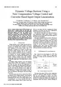
1. Introduction The effects of voltage dips, over-voltages and voltage harmonics on electric loads can be mitigated using DVRs. The general structure of a DVR can be seen in figure 1 where the it is connected to the sensitive load through an injection transformer [1]. The energy storage can be a group of batteries or a DC capacitor filtering the output of a diode rectifier conected to the electrical grid. The power converter switches at high frequency generating a PWM output voltage waveform which must be low-pass filtered (LF, RF and CF) before arrive to the injection transformer. Switches S1, S2 and S3 control the compensation status of the DVR [2]. The structure of the controllers applied to DVRs varies but in general, it can be divided in two fundamental blocks: the generation of the reference signal for the voltage injection, measuring the source (VS) or the load voltage, and the control of the output voltage to ensure that it corresponds to the reference signal, which considers the state variables in the LPF (IF and VF).
Fig. 1. Hardware structure of a DVR
The second block can be implemented in three ways. Feedback structures allow a good stationary response while forward structures generate quick responses during voltage transients. Feed-forward strutures allows both behaviours being more used [3]. The generation of the reference signal depends strongly on the compensation objectives: voltage dips, over-voltages or voltage harmonics. The rms value of the grid voltage can be measured to detect voltage dips and over-voltages, once detected, the PLL used to synchronize the compensation signal must be frozen (not applied to the voltage signal) to maintain the previous phase. When the load voltage harmonics are the compensation objective, a repetitive controller can be applied to mitigate the effect of all voltage harmonics [3]. In this case the reference signal is generated inside the voltage controller and doesn’t allow selective harmonic compensation, both in harmonic order and harmonic magnitude. Previously proposed methods for the control of DVRs operate in the time domain or in the frequency domain. Time domain methods have a fast dynamical response but don’t allow the selective compensation of voltage
disturbances. Methods based on the FFT allow the selection of the voltage disturbance to be compensated but have a slow dynamical response. This paper proposes a new digital technique which operates in the time and frequency domains, allowing selective compensation with fast dynamical response.
fundamental frequency voltage harmonic of order i, wk is the signal model noise vector and Mi is defined as:
2. Proposed Estimation Technique for the Generation of the Reference Signal
Being ω the angular frequency of the fundamental grid voltage harmonic component and TS the sampling time of the proposed discrete algorithm.
The structure of the proposed algorithm can be seen in figure 2. A stationary frame discrete Kalman filter obtains the amplitudes Vi of each voltage harmonic component [4]. These voltage harmonic components are used to establish the presence of a voltage disturbance comparing the measured values and the established operation values. Voltage dips and over-voltages are detected using the grid voltage fundamental harmonic component, the amplitudes of other measured voltage harmonic components are measured to establish the presence of harmonic distortion to be compensated. Once the DVR is switched-on using S1, S2 and S3, harmonic references Vi*(k) are obtained as difference of the measured voltage harmonic components and the desired ones.
The applied recursive discrete Kalman filtering loop corresponds to equations [5]:
⎛ cos(iωTs ) − sin(iωTs ) ⎞ ⎟⎟ M i = ⎜⎜ ⎝ sin(iωTs ) cos(iωTs ) ⎠
Pk |k −1 = APk −1|k −1 A T + Q k −1
(
G k = Pk |k −1C T CPk |k −1C T + R
Pk |k = (I − G k C)Pk |k −1
(3)
(4)
)
−1
(5) (6)
xˆ k |k −1 = Axˆ k −1|k −1
xˆ k |k = xˆ k |k −1 + G k (v Sk − Cxˆ k |k −1 )
(7) (8)
Where Pk|k+1 is the estimation of process covariance matrix at time instant k using its value at time instant k-1, Qk-1 is the variance matrix associated to vector wk, Gk is the Kalman gains matrix at time instant k, vector C, using this signal model, is defined as: C = (1 0 L 1 0 )
(9)
R is the variance matrix of the voltage measurement error ˆ k|k −1 is the prediction of voltage harmonic and x components in the stationary frame αβ at time instant k ˆ k −1|k −1 . using the estimation at time instant k-1 x The amplitude of the fundamental voltage harmonic component at instant k is evaluated as: V1 (k ) = V1α2 (k ) + V12β (k )
Fig. 2. Reference voltage estimator
The discrete Kalman filter uses a stationary frame voltage signal model, then, each voltage harmonic component at time instant k can be described as: x k +1 = Ax k + w k
(1)
which is compared with the required load voltage. When a voltage dip or over-voltage is detected the recursive Kalman filter is frozen at the fundamental frequency and the described filtering loop is reduced to eq. 7 at the fundamental harmonic component, using previously buffered values of V1α(k) and V1β(k). The compensation reference signal at the fundamental frequency is obtained as: V1* ( k ) =
Being: ⎛ V1α ⎞ ⎟ ⎜ ⎜ V1β ⎟ xk = ⎜ M ⎟ ⎟ ⎜ ⎜Vnα ⎟ ⎜V ⎟ ⎝ nβ ⎠ k
⎛ M1 0 L 0 ⎞ ⎟ ⎜ M ⎟ ⎜ 0 O A=⎜ M O 0 ⎟ ⎟ ⎜ ⎜ 0 L 0 M ⎟ n ⎠ ⎝
(2)
Where Viα and Viβ correspond respectively to the inphase and the in-quadrature components of the
(10)
V1R − V1 (k ) V1α (k ) V1R
(11)
where V1R is the required load voltage amplitude. The compensation references for higher order harmonic components of vs(k) are only applied when the established tolerance levels are reached. These signals are obtained as:
Vi * ( k ) =
Viα2 (k ) + Viβ2 (k ) − Vi R Viα ( k ) + Viβ ( k ) 2
2
V1α (k )
(3)
where ViR is the tolerate amplitude of the voltage harmonic of order i>1. Finally, the complete compensation reference signal at instant k can be obtained using: n
* V DVR ( k ) = ∑ Vi * ( k )
Figure 4 shows the obtained simulation results when a 30% over-voltage is applied at 100 ms. As it can be seen, once the over voltage is detected, the DVR acts reducing the load voltage amplitude to the load nominal voltage and the dynamical response takes 30 ms. This demonstrates that the proposed controller allows a properly compensation of over-voltages.
(4)
i =1
Where each Vi*(k) depends on the established tolerance level ViR , allowing the selective compensation of voltage disturbances
Finally, the voltage harmonic compensation capability of a DVR controlled using the proposed estimation reference technique is shown in figure 5. A grid voltage (vs) with a 5% of 5th harmonic component is applied. 500
The reference estimation technique has been applied using a sampling time of TS=156 μs and the grid voltage signal has been modeled using 1st, 3rd, 5th, 7th and 9th voltage harmonics, which correspond to the usual grid voltage harmonic content. The DVR has been modeled using a power converter with 400Vdc and a low-pass filter with LF=3 mH, RF=1.0 Ω and CF=230 µF. The nominal power of the injection transformer is 12 kVA with a primary and magnetization impedances of L1=0.17mH, R1=35mΩ, Lm=252mH and Rm=80Ω. The source voltage contains a 50Hz 325 V signal and a 5th harmonic of 5%.
250
0
−250
−500
0
20
40
60
80
100 Time (ms)
120
140
160
180
200
0
20
40
60
80
100 Time (ms)
120
140
160
180
200
500
Load Voltage (V)
The proposed algorithm has been tested in simulation, using the SimPowerSystems BlockSet from MatLab, according to figure 1.
Source Voltage (V)
3. Simulation Results
250
0
−250
−500
Fig. 4. Source and load voltages when a 30% over-voltage is applied 400
Source Voltage (V)
400
s
Voltage (V)
VL
0
−200
−400 320
330
340
360 Time (ms)
370
380
390
400
350 300
V
250
VL
s
200 150 100
0
0
100
200
0
300
400 500 Frequency (Hz)
600
700
800
900
Fig. 5. Source and load voltage waveforms and spectra for the 100% compensation of the 5th voltage harmonic.
−200
0
20
40
60
80
100 Time (ms)
120
140
160
180
200
The tolerance level for the 5th voltage harmonic (V5R) is fixed to 0 V for fully compensation. Obtained results show that the proposed control technique allows the 100% mitigation of the 5th voltage harmonic component.
400
200
0
4. Conclusions
−200
−400
350
50
200
−400
Load Voltage (V)
V 200
Amplitude (V)
A diode rectifier with a RC load (CL=1000µF, RL=500Ω) has been used as protected load. The obtained simulation results when the distorted grid voltage is applied can be shown in figure 3. The voltage dip is applied at t=100 ms being the voltage amplitude reduced to 195 V. The response time, including the voltage dip detection time and the controller response, is less than one cycle at the fundamental frequency which confirms the appropriate behavior of the proposed DVR control technique for the compensation of voltage dips.
0
20
40
60
80
100 Time (ms)
120
140
160
Fig. 3. Source and load voltage waveforms for a 40% voltage dip
180
200
A new digital control technique which applies a discrete Kalman filter to generate the compensation reference signal in DVRs has been presented and tested in simulation.
The structure of the proposed reference voltage estimator allows the compensation of voltage dips, over-voltages and voltage harmonics simultaneously. Moreover, the disturbance compensation degree can be fixed allowing a more flexible operation. Obtained simulation results allow to establish the appropriate dynamical and steady-state responses of the proposed estimation technique applied to DVRs.
References [1] [2]
[3]
[4]
[5]
J.G. Nielsen, Design and Control of a Dynamic Voltage Restorer, Ph.D. Thesis, Institute of Energy Technology, Aalborg University, Denmark. 2002. S. M. Silva, F. A. Eleutério, A. de Souza and B. J. Cardoso, “Protection Schemes for a Dynamic Voltage Restorer”, in Proc. of 39th IAS Annual Meeting, Vol. 4, pp 2239-2243. October 2004. Y. H. Cho and S. K. Sul, “Controller Design for Dynamic Voltage Restorer with Harmonics Compensation Function”, in Proc. of 39th IAS Annual Meeting, Vol. 3, pp 1452-1457. October 2004. V. Moreno and J. Barros, “Application of Kalman filtering for Continuous Real Time Tracking of Power System Harmonics”, IEE Proc.- Gener. Transm. Distrib. Vol. 144, No. 1, pp 13-20. January 1997. C. K. Chui and G. Chen, “Kalman Filtering with RealTime Applications” 3rd edition. Springer-Verlag. 1998.