Control of Hexapedal Pronking Through a Dynamically Embedded ...

CONTROL OF HEXAPEDAL PRONKING THROUGH A DYNAMICALLY EMBEDDED SPRING LOADED INVERTED PENDULUM TEMPLATE

A THESIS SUBMITTED TO THE GRADUATE SCHOOL OF NATURAL AND APPLIED SCIENCES OF MIDDLE EAST TECHNICAL UNIVERSITY

BY

MUSTAFA MERT ANKARALI

IN PARTIAL FULFILLMENT OF THE REQUIREMENTS FOR THE DEGREE OF MASTER OF SCIENCE IN ELECTRICAL AND ELECTRONICS ENGINEERING

FEBRUARY 2010

Approval of the thesis:

CONTROL OF HEXAPEDAL PRONKING THROUGH A DYNAMICALLY EMBEDDED SPRING LOADED INVERTED PENDULUM TEMPLATE

submitted by MUSTAFA MERT ANKARALI in partial fulfillment of the requirements for the degree of Master of Science in Electrical and Electronics Engineering Department, Middle East Technical University by,

¨ Prof. Dr. Canan Ozgen Dean, Graduate School of Natural and Applied Sciences Prof. Dr. ˙Ismet Erkmen Head of Department, Electrical and Electronics Engineering Asst. Prof. Dr. Afs.ar Saranlı Supervisor, Electrical and Electronics Engineering Dept., METU Asst. Prof. Dr. Uluc. Saranlı Co-supervisor, Computer Engineering Dept., Bilkent Uni.

Examining Committee Members: Prof. Dr. Aydan Erkmen Electrical and Electronics Engineering Dept., METU Asst. Prof. Dr. Afs.ar Saranlı Electrical and Electronics Engineering Dept., METU Prof. Dr. Kemal Leblebicio˘glu Electrical and Electronics Engineering Dept., METU ¨ Prof. Dr. Omer Morg¨ul Electrical and Electronics Engineering Dept., Bilkent University Asst. Prof. Dr. Emre Tuna Electrical and Electronics Engineering Dept., METU

Date:

I hereby declare that all information in this document has been obtained and presented in accordance with academic rules and ethical conduct. I also declare that, as required by these rules and conduct, I have fully cited and referenced all material and results that are not original to this work.

Name, Last Name:

Signature

:

iii

MUSTAFA MERT ANKARALI

ABSTRACT

CONTROL OF HEXAPEDAL PRONKING THROUGH A DYNAMICALLY EMBEDDED SPRING LOADED INVERTED PENDULUM TEMPLATE

Ankaralı, Mustafa Mert M.S., Department of Electrical and Electronics Engineering Supervisor

: Asst. Prof. Dr. Afs.ar Saranlı

Co-Supervisor

: Asst. Prof. Dr. Uluc. Saranlı

February 2010, 70 pages

Pronking is a legged locomotory gait in which all legs are used in synchrony, usually resulting in slow speeds but long flight phases and large jumping heights that may potentially be useful for mobile robots locomoting in cluttered natural environments. Instantiations of this gait for robotic systems suffer from severe pitch instability either due to underactuated leg designs, or the open-loop nature of proposed controllers. Nevertheless, both the kinematic simplicity of this gait and its dynamic nature suggest that the Spring-Loaded Inverted Pendulum Model (SLIP), a very successful predictive model for both natural and robotic runners, would be a good basis for more robust and maneuverable robotic pronking. In the scope of thesis, we describe a novel controller to achieve stable and controllable pronking for a planar, underactuated hexapod model, based on the idea of “template-based control”, a controller structure based on the embedding of a simple dynamical template within a more complex anchor system. In this context, high-level control of the gait is regulated through speed and height commands to the SLIP template, while the embedding controller based on approximate inverse-dynamics and carefully designed passive robot morphology ensures the stability of the remaining degrees of freedom. We show through extensive simulation experiments iv

that unlike existing open-loop alternatives, the resulting control structure provides stability, explicit maneuverability and significant robustness against sensor noise.

Keywords: hexapedal pronking, legged locomotion, spring loaded inverted pendulum (SLIP), embedding control, biologically inspired robotics

v

¨ OZ

¨ ULM ¨ ¨. ALTI BACAKLI PRONKLAMA DAVRANIS.ININ D˙INAM˙IK OLARAK GOM US ˙ ¨ YAYLI TERS SARKAC. S.ABLONU ILE KONTROLU

Ankaralı, Mustafa Mert Y¨uksek Lisans, Elektrik ve Elektronik M¨uhendisli˘gi B¨ol¨um¨u Tez Y¨oneticisi

: Yard. Doc¸. Dr. Afs.ar Saranlı

Ortak Tez Y¨oneticisi

: Yard. Doc¸. Dr. Uluc. Saranlı

S.ubat 2010, 70 sayfa

Pronklama, bacaklı mobil sistemlerde, b¨ut¨un bacakların senkronize bir s.ekilde kullanldı˘gı, genellikle g¨oreceli olarak d¨us.u¨ k hızlarda hareket eden, fakat uzun uc.us. s¨urelerine ve y¨uksek zıplama irtifalarına ulas.abilen bir davranıs. bic.imidir. Bu davranıs.ın robotik sistemlerdeki kullanımı, eksik eylem kapasitesine sahip bacak tasarımları ve varolan kontrolc¨ulerin ac.ık-d¨ong¨u tabanlı olmalarından dolayı, yunuslama hareketinde ciddi kararsızlık sorunlarını beraberinde getirmektedir. Bununla beraber, bu davranıs.ın kinematik ac.ıdan basit yapısı ve dinamik do˘gası, do˘gal veya robotik kos.ucular ic.in bas.arısı defalarca ortaya konmus. bir kestirimci model olan Yaylı Ters Sarkac. (YTS) modelinin daha g¨urb¨uz ve y¨uksek manevra kabiliyetine sahip bir pronklama davranıs.ını elde edebilmek ic.in temel olarak kullanılması fikrini desteklemektedir. Bu tez kapsamında, yapısal olarak basit fakat dinamik bir s.ablonun, daha karmas.ık bir dinamik sisteme g¨om¨ulmesi tabanına dayanan “s.ablon tabanlı kontrol” yapısının, kararlı ve manevra kabiliyeti y¨uksek bir pronklama davranıs.ını, eksik eylem g¨uc¨une sahip, dikey d¨uzlemde yas.ayan bir altı bacaklı robot modeli u¨ zerinde gerc.eklemek ic.in kullanıldı˘gı yeni bir kontrol algoritması gelis.tirdik. Bu ba˘glamda, y¨uksek seviyede c.alıs.an bir kos.ma kontrolc¨us¨u YTS s.ablonunun hız ve y¨ukseklik de˘gerlerini kontrol ederken, yaklas.ık ters dinamik vi

y¨ontemlerinin kullanımı ve dikkatlice tasarlanmıs. pasif yapısal o¨ zelliklerin varlı˘gına dayanan g¨omme kontrol¨u, kalan serbestlik derecelerinin kararlılı bir s.ekilde denetlenmesi ile ilgilenir. Kapsamlı sim¨ulasyon deneyleri aracılı˘gı ile, varolan ac.ık-d¨ong¨u tabanlı kontrolc¨uler ile kars.ılas.tırıldı˘gında, tasarlamıs. oldu˘gumuz bu yeni kontrol yapısının c.ok daha iyi kararlılık, manevra kabiliyeti ve kayda de˘ger derecede g¨urb¨uzl¨uk artıs.ı sa˘gladı˘gını g¨osterdik. Buna ek olarak, ciddi oranda algılayıcı ve denetim komut g¨ur¨ult¨us¨u altında kontrolc¨u performansının korundu˘gunu da genis. bir sim¨ulasyon yelpazesi ile g¨osterdik. Sonuc. olarak, daha o¨ nce hic.bir s.ekilde elde edilememis. bir pronklama davranıs. performansına ulas.mayı bas.ardık.

Anahtar Kelimeler: altı bacaklı pronklama, bacaklı hareketlilik, yaylı ters sarkac. (YTS), g¨omme kontrol, biyolojiden esinlenmeli robotik

vii

to my loving mother, to my beloved fianc´ee and to the memory of my dear father

viii

ACKNOWLEDGMENTS

I thank to my supervisors, Afs.ar Saranlı and Uluc. Saranlı, for their guidance, encouragement, and tremendous support throughout my M.S. study. They were always there to listen and give advice when I needed. I am very grateful to them for their patience during our research meetings and productive discussions, which carried me forward to this day both technically and morally. I took my initial steps into the area of bio-inspired robotics with SensoRHex Project, and I am thankful to all the members of the project. I would like to express my deep and sincere respect to Afs.ar Saranlı (the project manager), Uluc. Saranlı, Yi˘git Yazıcıo˘glu and Kemal Leblebicio˘glu for giving me the opportunity to be a part of this brilliant project environment. Especially, I would like to thank Uluc. Saranlı for inspiring me to legged locomotion with his endless energy and enthusiasm for legged systems. It has been his vision, enthusiasm and energy that helped me rediscover the enthusiasm and creativity that I had lost before. Maybe one of the most rewarding aspect of my M.S. study was the opportunity to work with the amazing group of people in Rolab (Laboratory of Robotics and Autonomous Systems), all helped me a lot along my way both technically and physiologically. I am very thankful to all members, especially to Emre Ege for his patience and endless support. Further thanks should also go to the all members of BDRL (Bilkent Dexterous Robotics and Locomotion), ¨ ur Arslan (my great colleague) for his undying enthusiasm and infinite stream especially to Om¨ of ideas. I also extend my thanks to my friends for their understanding and support during this thesis. I would also like to thank the Scientific and Technological Research Council of Turkey ¨ ˙ITAK) for awarding me their prestigious master of science studies scholarship. (TUB Finally, but forever I owe my loving thanks to my family, my loving mother (Sevinc. Ankaralı), my dear father (Barbaros Celalettin), Orhan Bes.er and my beloved fianc´ee (Ela Hast¨urk) for their undying love, support and encouragement.

ix

TABLE OF CONTENTS

ABSTRACT . . . . . . . . . . . . . . . . . . . . . . . . . . . . . . . . . . . . . . . .

iv

¨ . . . . . . . . . . . . . . . . . . . . . . . . . . . . . . . . . . . . . . . . . . . . . OZ

vi

DEDICATION . . . . . . . . . . . . . . . . . . . . . . . . . . . . . . . . . . . . . . viii ACKNOWLEDGMENTS . . . . . . . . . . . . . . . . . . . . . . . . . . . . . . . . .

ix

TABLE OF CONTENTS . . . . . . . . . . . . . . . . . . . . . . . . . . . . . . . . .

x

LIST OF TABLES . . . . . . . . . . . . . . . . . . . . . . . . . . . . . . . . . . . . xiii LIST OF FIGURES . . . . . . . . . . . . . . . . . . . . . . . . . . . . . . . . . . . . xiv CHAPTERS 1

2

INTRODUCTION . . . . . . . . . . . . . . . . . . . . . . . . . . . . . . .

1

1.1

Motivation and Background . . . . . . . . . . . . . . . . . . . . . .

1

1.2

Existing Work . . . . . . . . . . . . . . . . . . . . . . . . . . . . .

4

1.3

Methodology and Contributions . . . . . . . . . . . . . . . . . . . .

6

1.4

Organization of the Thesis . . . . . . . . . . . . . . . . . . . . . . .

7

THE PLANAR SPRING LOADED INVERTED PENDULUM . . . . . . . .

8

2.1

The Basic SLIP Model and Dynamics . . . . . . . . . . . . . . . . .

9

2.1.1

SLIP Dynamics . . . . . . . . . . . . . . . . . . . . . . .

9

2.2

Dimensionless System Model and Dynamics . . . . . . . . . . . . .

10

2.3

Control of SLIP Locomotion . . . . . . . . . . . . . . . . . . . . .

12

2.3.1

SLIP Control Inputs . . . . . . . . . . . . . . . . . . . .

12

2.3.2

Analytical Approximate Stance Maps . . . . . . . . . . .

13

2.3.2.1

Approximate Stance Map by Saranli . . . . .

14

2.3.2.2

Approximate Stance Map by Geyer et al. . . .

16

Deadbeat Gait Control of SLIP Locomotion . . . . . . . .

17

2.3.3

x

2.4

The SLIP Model with Damping . . . . . . . . . . . . . . . . . . . .

19

2.4.1

System Model and Dynamics . . . . . . . . . . . . . . . .

19

2.4.2

A New Analytical Approximate Stance Map for SLIP Model with Damping . . . . . . . . . . . . . . . . . . . . . . . . 20 2.4.2.1

Approximating Stance Trajectories under Damping . . . . . . . . . . . . . . . . . . . . . . . 20

2.4.2.2

Times of Critical Events: Bottom and Liftoff .

22

2.4.2.3

Energy Based Correction on Liftoff States . .

24

Simulation Results for the Lossy SLIP Model . . . . . . .

24

2.4.3.1

Predictive Performance . . . . . . . . . . . .

24

2.4.3.2

Tracking Performance . . . . . . . . . . . . .

26

Conclusion . . . . . . . . . . . . . . . . . . . . . . . . . . . . . . .

27

The Torque Actuated Spring Mass Hopper . . . . . . . . . . . . . . . . . . .

29

3.1

System Model and Dynamics . . . . . . . . . . . . . . . . . . . . .

29

3.2

Template Control of SLIP-T Locomotion . . . . . . . . . . . . . . .

32

3.2.1

Virtual Foot Placement and Virtual Toe Coordinates . . . .

32

3.2.2

Control of SLIP-T Stance Dynamics . . . . . . . . . . . .

33

3.2.3

Gait Level Control of SLIP-T Locomotion . . . . . . . . .

34

Simulation Studies . . . . . . . . . . . . . . . . . . . . . . . . . . .

37

3.3.1

Existence and Stability of Limit Cycles . . . . . . . . . .

37

3.3.2

Stability and Basins of Attraction . . . . . . . . . . . . .

38

3.3.3

Maneuverability . . . . . . . . . . . . . . . . . . . . . . .

39

Conclusion . . . . . . . . . . . . . . . . . . . . . . . . . . . . . . .

39

CONTROL OF HEXAPEDAL PRONKING . . . . . . . . . . . . . . . . . .

41

4.1

Background: Slimpod - A Planar Hexapod Model . . . . . . . . . .

41

4.1.1

System Model and Assumptions . . . . . . . . . . . . . .

41

4.1.2

Dimensionless Dynamics . . . . . . . . . . . . . . . . . .

43

4.1.2.1

Mode Transitions . . . . . . . . . . . . . . .

44

Template Control of Planar Hexapedal Pronking . . . . . . . . . . .

45

4.2.1

46

2.4.3

2.5 3

3.3

3.4 4

4.2

Control of Slimpod Stance Dynamics . . . . . . . . . . . xi

4.2.1.1

Handling Singularities, Torque Limits and Partial Stance . . . . . . . . . . . . . . . . . . .

47

Gait Level Control of Embedded Slimpod Model . . . . .

49

Simulation Studies . . . . . . . . . . . . . . . . . . . . . . . . . . .

50

4.3.1

Existence and Nature of Stable Limit Cycles . . . . . . . .

51

4.3.2

Stability and Basins of Attraction . . . . . . . . . . . . .

52

4.3.3

Maneuverability . . . . . . . . . . . . . . . . . . . . . . .

53

4.3.4

Sensitivity Analysis . . . . . . . . . . . . . . . . . . . . .

56

4.3.5

Sensitivity to Parameter Uncertainty . . . . . . . . . . . .

57

4.3.6

Sensitivity to Discrete Control and Sensor Noise . . . . .

58

Conclusion . . . . . . . . . . . . . . . . . . . . . . . . . . . . . . .

61

CONCLUSION . . . . . . . . . . . . . . . . . . . . . . . . . . . . . . . . .

62

5.1

Future Work . . . . . . . . . . . . . . . . . . . . . . . . . . . . . .

63

REFERENCES . . . . . . . . . . . . . . . . . . . . . . . . . . . . . . . . . . . . . .

64

4.2.2 4.3

4.4 5

APPENDIX A

DERIVATION OF THE JACOBIANS FOR THE SLIMPOD MODEL . . . .

69

A.1

69

Derivation of the Jacobians . . . . . . . . . . . . . . . . . . . . . .

xii

LIST OF TABLES

TABLES

Table 2.1 State variables, parameters and the definitions of their dimensionless counterparts for the basic SLIP model. Variables with and without bars correspond to physical and dimensionless quantities, respectively. . . . . . . . . . . . . . . . .

11

Table 2.2 Computation of leg length control inputs ξtd and ξlo . . . . . . . . . . . . .

18

Table 2.3 Average percentage prediction errors for both Geyer’s and our methods in predicting various elements of the SLIP state. . . . . . . . . . . . . . . . . . . . .

25

Table 3.1 State variables, parameters and the definitions of their dimensionless counterparts for the SLIP-T model. . . . . . . . . . . . . . . . . . . . . . . . . . . . .

30

Table 3.2 Kinematic and Dynamic Parameters of the SLIP-T Model . . . . . . . . . .

37

Table 4.1 Variables, parameters and the definitions of their dimensionless counterparts for the Slimpod model. . . . . . . . . . . . . . . . . . . . . . . . . . . . . . . .

43

Table 4.2 Kinematic and Dynamic Parameters of the Slimpod Model . . . . . . . . .

51

Table 4.3 Sensitivity of steady-state tracking errors to sensory noise on different state variables. β and γ are slopes and offsets of a linear relation between the standard deviation of the steady state error and the standard deviation of the noise. . . . . .

xiii

60

LIST OF FIGURES

FIGURES

Figure 1.1 Snapshot of a planar hexapedal pronking stride . . . . . . . . . . . . . . .

3

Figure 1.2 Gazelle pronking [1] . . . . . . . . . . . . . . . . . . . . . . . . . . . . .

4

Figure 2.1 The Spring-Loaded Inverted Pendulum Model . . . . . . . . . . . . . . .

9

Figure 2.2 SLIP locomotion phases (shaded regions) and transition events (boundaries) 10 Figure 2.3 The Spring-Loaded Inverted Pendulum Model with Damping . . . . . . .

19

Figure 2.4 Left: Average apex position prediction performance as a function of damping. Right: Average total mechanical energy prediction performance as a function of damping. The vertical bars represent the corresponding standard deviation. . .

25

Figure 2.5 Left: Average apex position prediction performance as a function of damping. Right: Average total mechanical energy prediction performance as a function of damping. Error axes are plotted in logarithmic scale to simultaneously show the predictive performances of Geyer’s approximations with the proposed method, which yields mean errors that are two orders of magnitude better than its alternatives. 26 Figure 2.6 Comparison of apex forward speed (left) and height (right) mean tracking errors at steady-state for a spring-mass runner with different damping coefficients in the leg. . . . . . . . . . . . . . . . . . . . . . . . . . . . . . . . . . . . . . . .

27

Figure 3.1 SLIP-T : Spring-mass hopper with a fully passive leg and a rotary hip actuation . . . . . . . . . . . . . . . . . . . . . . . . . . . . . . . . . . . . . . .

29

Figure 3.2 An example SLIP-T simulation with tend = 30 (t¯end = 4.2s for SensoRHex), starting from an initial condition of z = 1.4, y˙ = 0.9, towards an apex goal z∗ = 1.1, y˙ ∗ = 1.1. . . . . . . . . . . . . . . . . . . . . . . . . . . . . . . . . . . . . . . . xiv

38

Figure 3.3 Stable domain of attraction for the SLIP-T model towards the goal y˙ ∗a = 1.1 and z∗a = 1.16. The green region shows initial conditions from which locomotion converges to a stable limit cycle. Dashed lines illustrate a few example runs to show convergence behavior. . . . . . . . . . . . . . . . . . . . . . . . . . . . . .

39

Figure 3.4 Maneuverability of the SLIP-T controller. The blue region illustrates the set of apex goal settings for which stable pronking is possible and steady-state was within 5% of the desired goal. . . . . . . . . . . . . . . . . . . . . . . . . . . . .

40

Figure 4.1 Slimpod: A planar dynamic model for hexapedal pronking . . . . . . . . .

42

Figure 4.2 Leg kinematics at the time of touchdown . . . . . . . . . . . . . . . . . .

50

Figure 4.3 An example pronking simulation with tend = 30 (t¯end = 4.2 s for RHex), starting from an initial condition of z = 1.4, y˙ = 0.9, α˙ = 0, towards an apex goal z∗ = 1.1, y˙ ∗ = 1.1. . . . . . . . . . . . . . . . . . . . . . . . . . . . . . . . . . .

52

Figure 4.4 Torque Profiles of the Slimpod Model for a Single Stance Phase at Steady State . . . . . . . . . . . . . . . . . . . . . . . . . . . . . . . . . . . . . . . . .

53

Figure 4.5 Cross section (˙ya -za ) of the domain of attraction towards the goal y˙ ∗a = 1.1 and z∗a = 1.16. The shaded green region illustrates initial conditions from which the hexapod converges to stable pronking. Dashed lines illustrate a few example runs to show convergence behavior. . . . . . . . . . . . . . . . . . . . . . . . . .

54

Figure 4.6 Cross section (α˙ a -za ) of the stable domain of attraction towards the goal y˙ ∗a = 1.1 and z∗a = 1.16. The shaded green region illustrates initial conditions from which the hexapod converges to stable pronking. Dashed lines illustrate a few example runs to show convergence behavior. . . . . . . . . . . . . . . . . . . . .

54

Figure 4.7 Maneuverability of the pronking controller. The shaded blue region illustrates the set of apex goal settings for which stable pronking is possible and steady-state was within 5% of the desired goal. . . . . . . . . . . . . . . . . . . .

55

Figure 4.8 Pronking Slimpod model following a time varying desired apex trajectory. Blue pluses illustrates the progression of apex states with respect to time. Red lines indicate the desired apex state trajectories. . . . . . . . . . . . . . . . . . .

56

Figure 4.9 Sensitivity of steady-state tracking performance of the pronking controller with respect to a miscalibrated relative spring stiffness κˆ i . . . . . . . . . . . . . . xv

57

Figure 4.10 Sensitivity of steady-state tracking performance of the pronking controller with respect to a miscalibrated horizontal COM position. xCOM − xˆCOM > 0 means that the actual COM is ahead of its position assumed by the controller. . . . . . .

xvi

59

CHAPTER 1

INTRODUCTION

1.1

Motivation and Background

At present, there are already many existing mobile platforms, such as wheeled or tracked vehicles, which provide sufficient robustness, high speeds and energetic performance for many applications. On the other hand, one must also consider that the performance of these traditional mobile robots largely results from the structured nature of their operating environments. Increasing demand for robots to operate for different applications is beginning to show the limitations of wheeled and tracked systems due to the fact that they have restricted motion capabilities over unstructured and rough surfaces [41]. Robotic mobility over highly broken and unstable terrain surely requires legged platforms. Despite several effective behaviors and performance demonstrated by tracked and wheeled vehicles [64, 58], the repertoire of behaviors realizable with such morphologies inevitably remains limited due to restricted directions in which forces can be applied to the robot body. Consequently in the long run, systems capable of operating in the widest variety of terrain conditions, will be legged robots. In [23] and [47], the disadvantages of wheels compared to the legs were discussed. They say that the efficiency of wheels is restricted to flat surfaces, with application areas mostly limited to structured arenas (e.g roads and rails) since some limited natural settings and they have limited motion capabilities in the presence of vertical obstacles. On the other hand, legged robot morphologies admit a wider range of behavioral alternatives than more traditional tracked or wheeled platforms with added mobility provided by otherwise infeasible behaviors such as running [6], leaping and self-righting [54]. There are many outstanding and challenging 1

examples of locomotion that can be achieved by using legs, but are difficult or sometimes impossible for wheels. For instance, a good example is the RISE robot, a biologically inspired hexapedal climbing platform capable of locomotion on different vertical structures such as walls and trees [62, 57, 10]. Another example of the challenging environments for robots are sandy terrains wherein wheeled robots usually get stuck. However, SandBot, a bio-inspired hexapedal robot, can impressively traverse over sand [31]. Even though we can easily conclude that legged robots can reach all regions that animals can travel on foot (hypothetically), legged systems present many difficulties to engineers in their design and control. Unlike traditional mobile robots, legged systems suffer from additional hardware complexity to support leg mechanisms. During the design of legged robots, engineers have to increase the number of actuators to increase the freedom of movement while sacrificing reliability. With this increased kinematic complexity and decreased reliability, stable and efficient locomotion may become impossible due to physical (bandwidth, reliability etc.) limitations with today’s technology. Another difficulty that comes with legs is that, unlike traditional mobile robots, control of locomotion with these platforms is very difficult and requires a thorough understanding of their dynamics and mechanical structure. The coordination of large degrees of freedom and redundancy in actuated joints compared to the small number of task degrees of freedom, present important challenges in the design of locomotion controllers for legged robots. A simple solution to these problems has been adopted by many legged robots through statically stable gaits, keeping their center of mass within the support area of the legs [14, 25]. The effectiveness of this method is limited by the necessity of operating at very low speeds, where the kinematics dominate the behavior. The effective actuation bandwidth is thus limited by sacrificing speed for force, while considerably decreasing energy efficiency. Moreover, the possibility of dynamic gaits is eliminated due to the stiff coupling of actuators to the environment, since impacts and collisions with the environment is inevitable. A similar way of controlling legged robots is by keeping the Zero Moment Point (ZMP) within the support are of the legs, in which velocities are also taken into account [37, 36]. However this method also suffers from many of the above problems. If we look at nature, we can see that the speed and agility of animals results from their efficient and dynamically dexterous use of their bodies. Consequently, nature tells us that a good 2

way in which this mechanical complexity can be decreased while increasing the performance of robots is the use of dynamic modes of locomotion, wherein second order dynamics are properly designed, tuned and exploited to achieve a wide variety of behaviors even in the absence of full actuation [4, 56, 54]. Early instantiations of this idea can be found in Raibert’s runners [47], capable of fast and stable locomotion over rough terrain despite being severely underactuated. In practice, this approach also has the advantage of significantly improving robustness and decreasing power requirements as a result of using fewer actuators and the associated reduction in weight and complexity [52]. Even though for tasks where, precision is required, static stability may become desirable, it cannot match the speed and efficiency that a dynamical mode of operation can achieve [52, 42]. Unfortunately, the design, analysis and control of such dynamically dexterous legged platforms is more challenging than simpler but slow, statically stable platforms due to difficulties in understanding and controlling second order dynamics. Despite substantial research in this domain, sufficiently general solutions to this problem remain elusive.

90

90 90

90

0 90

90

90

90

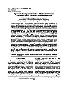
Figure 1.1: Snapshot of a planar hexapedal pronking stride

In this thesis, we present the mathematical basis and a practical implementation of template based control of dynamic legged locomotion, a controller structure based on the embedding of a simple dynamical “template”(SLIP) within a more complex “anchor” system [29]. We concentrate on the pronking behavior for the hexapedal RHex platform [52], whose robust and consistent realization in the absence of radial leg actuation has previously not been possible [43]. Pronking (aka. stotting) is a running gait adopted by legged animals in which all legs are used in synchrony and a substantial flight phase is induced (see Fig. 1.1). Pronking is rarely used for running any distance, but llamas, deer, impalas, gazelles and springboks all use pronking 3

(see Fig. 1.2), often to signal their strength to potential predators [28, 15]. In [61], it has been suggested that increased ground clearance in pronking may be useful both for seeing further, and for disseminating warning scents when predators are near. Even though such goals are unnecessary for robotic platforms, large jumping heights associated with this gait are potentially useful for locomotion on cluttered natural environments and may even increase efficiency by decreasing damping losses. Moreover, the lateral symmetry of the gait admits the use of simpler, planar models and provides a rich domain for studying feedback control of dynamic legged locomotion, particularly in the presence of underactuated leg structures. Such a planar simplification also allows the analysis of similar gaits such as the trot and the pace [11].

Figure 1.2: Gazelle pronking [1]

1.2

Existing Work

There has been very little explicit focus on robotic pronking in the literature [43, 11, 19, 45], as opposed to the much more widely studied bounding behavior [49, 46, 67, 18]. In several existing robots, fully actuated leg designs are used. Despite advantages in mobility and ease of control offered by such morphologies, the associated electromechanical complexity significantly impairs performance for autonomous outdoor tasks and dynamic behaviors, [45]. In contrast, robots with carefully designed passive compliant dynamics showed that a large 4

pallet of behaviors are still possible with very few actuators [4, 47, 56]. Consequently, our emphasis in this thesis is on how robust and maneuverable pronking can be obtained with similarly underactuated robots, in particular, the RHex hexapod [52]. Regardless of available actuation, stable and maneuverable control of pronking is a difficult problem. Existing control strategies for pronking (as well as bounding) largely rely on openloop strategies (e.g. with constant hip torque inputs or open-loop leg angle profiles) that offer little or no control authority over high level gait parameters and require extensive tuning to be successful. Even though the use of optimization methods promises to yield some insight into useful design criteria for robots capable of such highly dynamic behaviors [17], the range of operation and extensibility of resulting controllers remains limited. Moreover, many of these open-loop controllers suffer from severe pitch instability and even the addition of low-bandwidth sensory components does not yield sufficient robustness for autonomous operation [43]. In fact, pronking dynamics under simple energy-based feedback and largely open-loop leg control was shown to be inherently unstable for certain ranges of body inertia and locomotion heights [12]. In this context, there is significant biological [24, 39] and engineering [40, 38] evidence to support the adoption of predominantly open-loop controllers with properly tuned passive dynamics and minimal feedback for reliable locomotion. Nevertheless, high-bandwidth feedback controllers based on accurate dynamic models of such systems are still necessary for the insight they provide into the design of both the mechanism and its control. Among successful examples are use of zero dynamics for the stabilization of walking and running behaviors [63, 21] as well as self-righting behaviors for the RHex hexapod [54], both of which use sufficiently accurate dynamical models and subsequent high-bandwidth feedback to achieve stable and dynamic locomotory behaviors. Our contributions in this thesis not only provide a decompositional method that simplifies the design of such controllers, but also illustrate performance and maneuverability benefits associated with the use of model-based feedback control. There is also a large body of literature studying simpler, more fundamental models for basic locomotory behaviors, motivating our adoption of the Spring-Loaded Inverted Pendulum (SLIP) model. This model has received substantial attention in the literature, starting from its biological foundations [13, 27], leading to its instantiation within dynamically dexterous

5

monopods [47, 33], followed by subsequent analysis [59, 5, 55] and the design of associated gait controllers. Our treatment of the SLIP model also benefits from our recent work on its control through analytical return maps [9, 7].

1.3

Methodology and Contributions

Our method is based on decomposing system degrees of freedom into two components: A dynamical “template”, handling degrees of freedom most relevant for the description and control of the high level task, and the “anchor”, encompassing the remaining degrees of freedom representing the specific morphology of the system. In this context, high-level control of the gait is regulated through speed and height commands to the SLIP template, while the embedding controller based on approximate inverse-dynamics and carefully designed passive dynamics ensures the stability of the remaining degrees of freedom. Due to sensory limitations of our experimental platform, we use a non-dimensional, previously validated planar simulation to provide a careful and thorough characterization of the stability properties and noise performance of the proposed pronking controller. Our primary contribution in this thesis is the application of the template-based control idea, presented in [51] in the context of alternating tripod running, to dynamic pronking, while also providing a much more careful characterization of its stability properties and robustness against model and measurement uncertainty. Our extensions and improvements to the existing ideas makes the stability and maneuverability properties of our controller superior to those that were obtained for alternating tripod gaits in [51, 53]. We use extensive simulation studies to show that unlike existing open-loop alternatives, the resulting control structure provides explicit maneuverability and significant robustness against model, sensor and actuator noise. In addition to the main contributions of the thesis, as a by-product we developed a new analytical approximation to the stance dynamics of the Spring-Loaded Inverted Pendulum model that also takes into account non-negligible damping in the leg. 6

1.4

Organization of the Thesis

In the first part of the thesis in Chapter 2, we start with the introduction of the SLIP model. We give the necessary background including assumptions, dynamics and associated terminology. Later in Section 2.2, we nondimensionalize the equations of motion of the model to obtain the dynamics that are free from units. Subsequently, in Section 2.3, we give details about control of SLIP locomotion and make an overview of two existing approximations that are derived for its stance map. At the end of Chapter 2 we introduce the SLIP model with damping and derive a new analytical approximation method that also takes into account damping in the leg. We then present in Chapter 3, our embedding control framework in the context of a onelegged system that captures most relevant actuator limitations in the RHex platform except the pitch degree of freedom. Finally, we proceed with the pronking controller for the full planar hexapod model in Chapter 4.

7

CHAPTER 2

THE PLANAR SPRING LOADED INVERTED PENDULUM

In late-1970’s, biomechanists discovered the Spring-Loaded Inverted Pendulum (SLIP) model, illustrated in Fig. 2.1, as a metaphor for running animals [3]. Subsequent research in biomechanics established the SLIP model as a very accurate descriptive model for running animals of widely differing sizes and morphologies as diverse as humans and cockroaches [2, 13, 26]. In parallel, the same model was also used as the basis of numerous robots capable of dynamic locomotion such as Raibert’s hoppers [47], the ARL-Monopods [33], the Bow-Leg hopper [65], the BiMASC robotic leg [35] etc. These developments and growing biological evidence led to an increasing belief that the SLIP model may be more than just a descriptive model that fits biological data, but also a literal control target whose dynamics are an effective and appropriate goal for running behaviors [29]. Evidence to this end was provided by Raibert’s robots as well as work on active embedding of SLIP dynamics within more complex morphologies [6, 51, 55]. The main scope of this thesis is also included in this group. Nevertheless, despite the apparent simplicity of this model, it presents difficulties from an engineering point of view to conduct formal analysis and design control algorithms. SLIP is a hybrid dynamical system with nonlinear stance dynamics that are not integrable in closedform under the effect of gravity [34] , motivating a number of analytical approximations to support the analysis of its behaviors and the design of associated controllers [59, 51, 30, 9, 7]. We continue this chapter with the basic SLIP model and associated terminology. We then give details about a particular type of SLIP control method and summarize two previous approximate analytical stance maps. Finally, we introduce the SLIP model with damping and derive a new analytical approximation method that also takes into account damping in the leg.

8

2.1

The Basic SLIP Model and Dynamics

Figure 2.1: The Spring-Loaded Inverted Pendulum Model

Fig. 2.1 illustrates the the basic planar SLIP model, consisting of a point mass m attached to a freely rotating massless leg, with compliance of k s and rest length of l0 . Throughout locomotion, the system alternates between stance and flight phases. Due to the hybrid nature of this model, its continuous dynamics change depending on the state of ground contact. During flight, the body is assumed to be a projectile acted upon by gravity,whereas in stance, the leg is free to rotate around its toe (assumed to be fixed on the ground) with the body mass feeling radial forces induced by the leg. Moreover, the stance phase is further decomposed into two subphases, compression and decompression. Similarly, the flight phase is decomposed into the ascent and descent subphases. Four important events define transitions between these subphases: touchdown, as the leg comes into contact with the ground, marking the transition from flight to stance; bottom, as the leg reaches its maximal compression during stance phase; liftoff, as the toe takes off from the ground and finally apex, as the body reaches its maximum height during flight. Fig. 2.2 shows a single stride starting from an apex state and labels all relevant phases and transition events. Furthermore, Table 2.1 details all relevant variables and parameters for the basic SLIP model.

2.1.1 SLIP Dynamics

In flight, the dynamics of the system are those of a point mass acted upon by gravity which has a well known analytical solution. Using the parameters detailed in Table 2.1 we write the 9

Figure 2.2: SLIP locomotion phases (shaded regions) and transition events (boundaries) flight dynamics of the model in cartesian coordinates as      y¨¯   0        =   . z¨¯ −g 

(2.1)

During the stance phase, the dynamics of the system are those of an inverted compliant pendulum whose hinge is assumed to be fixed on the ground. The dynamics of the model in polar leg coordinates take the form     ξ¨¯   ξ¯ ψ˙¯ 2 − k /m(ξ¯ − l ) − g cos ψ¯ s 0     =   ¯ ξ¯ ψ¨¯ (−2 ξ˙¯ ψ˙¯ + g sin ψ)/

2.2

    .

(2.2)

Dimensionless System Model and Dynamics

Nondimensionalization is the removal of units from an equation set involving physical quantities by a suitable substitution of variables. Nondimensionalization can be applied to all quantitive models and it offers an efficient way to interpret complex data sets, i.e. simulation and experimental data, because usually the physical models in their original form are rather general. Formulation of systems with dimensionless variables simplifies and parametrizes problems, thus making subsequent analysis easier and more useful. In order to eliminate redundant parameters and provide an efficient way to interpret our simulation results, we will 10

Physical Quantity t¯ [ y¯ , z¯ ] ¯ ψ¯ ] [ ξ, v¯ [ z¯a , y˙¯ a ] ks F¯ E¯ p¯ ψ¯

Dimensionless Group t [ y, z ] [ ξ, ψ ] v [ za , y˙ a ] κs F E pψ

Definition := t¯ /λ := [ y¯ /l0 , z¯/l0 ] ¯ 0 , ψ¯ ] := [ ξ/l := v¯ (λ/l0 ) := [ z¯a /l0 , y˙¯ a (λ/l0 ) ] := k s (l0 /(mg)) := F¯ /(mg) := E¯ /(mgl0 ) := p¯ ψ¯ (λ/(ml02 ))

Description p Time (where λ := l0 /g) Body position SLIP leg length and leg angle Body Speed Apex height and velocity SLIP leg spring stiffness Force variables Energy variables Angular momentum

Table 2.1: State variables, parameters and the definitions of their dimensionless counterparts for the basic SLIP model. Variables with and without bars correspond to physical and dimensionless quantities, respectively.

use a dimensionless formulation of the dynamics both for the SLIP model and subsequent, more complex models. Previously, several researchers used dimensionless formulations in oder to define the dynamics of legged systems (e.g. [18]) and our methodology will be similar to them. We start our dimensionless formulation by redefining time as t := t¯/λ with λ :=

p

l0 /g.

After that, scaling all distances with the spring rest length l0 and using definitions detailed in Table 2.1, we write the SLIP dynamics in dimensionless coordinates as

Flight:

Stance:

     y¨   0        =   , z¨ −1      ξ¨   ξ ψ˙ 2 − cos ψ − κ (ξ − 1) s     ¨  =  (−2 ξ˙ ψ˙ + sin ψ)/ξ ψ

(2.3)     .

(2.4)

Note that (d/dt)n = λn (d/dt¯)n and all time derivatives in the above equations are with respect to the newly defined, scaled time variable. Throughout the rest of the thesis, we will only work with dimensionless quantities and hence will not explicitly mention their dimensionless nature unless necessary. 11

2.3

Control of SLIP Locomotion

In this section we will discuss the control objective of the SLIP model and how this objective can be achieved. For SLIP models and SLIP inspired robotic platforms the control objective is generally the regulation of apex states of the model during the locomotion. In order to formalize the control objective, we first define the set of controllable apex states as n o Xa = Xa | Xa = [ y˙ a , za ]T .

(2.5)

Then a relation between successive apex states can be formed as Xa [n + 1] = fa (Xa [n], U[n]) ,

(2.6)

where fa is the apex return map and U is the discrete control inputs of the SLIP model. Details about control inputs will be explained in Section 2.3.1. Suppose that we want to reach the desired apex states,    y˙∗   a  . X∗a =   z∗  a

(2.7)

Then the control objective is identifying the sequence of control inputs, {U[i])}ni=0 , to asymptotically converge to the desired apex states, X∗a .

2.3.1 SLIP Control Inputs

In the control of SLIP locomotion, there are two main control parameters that are common to all SLIP models and spring-mass hopping robots. These are the touchdown leg angle, ψtd , and the amount of change in the total mechanical energy, ∆E. The first control parameter, ψtd , is conceptually simple and corresponds to the control of the leg angle during flight such that at the instant of touchdown, the required leg angle is achieved. However, energy control of SLIP hopping can be achieved with a variety of different control inputs [59, 65, 51]. A good and detailed explanation of these control inputs and corresponding explanations can be found in [8]. In the scope of this thesis, we use leg lengths at touchdown ξtd and liftoff ξlo as the remaining two control inputs. This choice offers several advantages. Firstly, it makes the stance phase fully passive, allowing much simpler and more robust mechanical robot designs, 12

simplifying controller designs etc. An exact realization of this control policy is Zeglin’s Bow leg hopper [66], where a curved compliant leg is used, together with a tunable extension limit mechanism on the leg that satisfies precompressing the leg before touchdown (ξtd ) and limiting the leg to achieve premature liftoff (ξlo ). As mentioned in Chapter 1 our actual aim of analyzing the SLIP model is its use as a control target for our hexapod robot platform, SensoRHex, through embedding of its ideal dynamics. Since our target platform, SensoRHex, does not have tunable leg springs and its actuators lack radial actuation affordance [51], adjustment of the leg spring stiffness from compression to decompression is not a possible alternative for our SLIP controller that will work behind the hexapod model. It is also clear that we can not adjust touchdown and liftoff leg lengths with the fully passive physical legs of the RHex. However, as we will describe in later chapters, our embedding controller is based on the definition of a virtual SLIP, whose toe virtual toe admits us to arbitrarily control its leg length at touchdown. A similar choice was made in the earlier work for the template based control of tripod running [53]. To summarize, the set of SLIP control inputs we use in this thesis is defined as n o U = U | U = [ ψtd , ξtd , ξlo ]T ,

(2.8)

2.3.2 Analytical Approximate Stance Maps

Earlier researchers implemented intuitive and simple controllers for the locomotion of SLIP model and SLIP-like robotic platforms [48]. Even though these controllers generally had a good performance to stabilize locomotion, their performance were very limited in terms of tracking accuracy, basins of attraction etc. It is clear that we need more information than intuition alone about the nature of the apex return map defined in (2.6) in order to design high performance gait controllers and obtain insights about the stability properties of SLIP locomotion. The best way to do this is to obtain an analytical expression for the apex return map, fa . One needs to solve both the flight and stance dynamics of the model to obtain such an expression. The analytical solution of flight dynamics is very simple since the body follows a ballistic trajectory. The solution details about the flight dynamics can be found in [8, 51]. Unfortunately, despite the structural simplicity of the SLIP model, its stance dynamics are not integrable [34]. Consequently, there are no exact analytical expressions for the stance map and 13

consequently for fa . In order to overcome this problem, several researchers designed several controllers based on numerical solutions of the SLIP dynamics or empirical data captured from running videos of legged robots or animals [16]. These methods were very inaccurate and computationally inefficient to designing control policies, also they provide very limited information about the nature of the apex return map. It seems that approximate analytical solutions to nonintegrable stance dynamics are the best solutions to this problem. In the literature, there are a number of accurate analytic approximate stance maps to support the analysis of SLIP locomotion and the design of associated controllers and planning algorithms [59, 51, 30, 9]. The general idea behind approximate stance maps is the estimation of the all liftoff states, given the touchdown states. On the other hand, for a given initial apex state, Xa [n], touchdown states are calculated solving the flight dynamics and using selected set of control inputs, U[n], as boundary conditions. In the following sections, two previous analytical approximate stance maps, [51] and [30], are summarized and modified to be consistent with our dimensionless notation and selected set of control inputs.

2.3.2.1 Approximate Stance Map by Saranli

In this section, we will review the the analytical approximate stance map by Saranli [51], which is a modified version of the stance map developed by Schwind et. al. [60]. The summary of the stance map with our dimensionless variables is presented below. Suppose that necessary touchdown parameters, ξtd , ψtd , ξ˙td , ψ˙ td , are known. We can then calculate the body speed, vtd , and angular momentum, pψ td , at touchdown. After that, the total mechanical energy of the system at touchdown is found as Es =

vtd 2 + Uˆ g (ξtd ) , 2

(2.9)

where Uˆ g (ξtd ) is the approximated potential energy. This stance map uses the linearized gravity approximation where the true potential energy Ug (ψ, ξ) :=

κs (ξ − 1)2 + ξ cos ψ , 2 14

(2.10)

is approximated by κs Uˆ g (ξ) := (ξ − 1)2 + ξ . 2

(2.11)

The next step is calculating the bottom leg length, ξb , of the spring. We assume that along the stance period angular momentum of the body is conserved such that pψ ≈ pψ td . Using this assumption and the conservation of mechanical energy we obtain pψ 1 1 Es ξb 4 + ( − 1)ξb 3 + ( − )ξb 2 + = 0. 2 κs 2 κs 2κ s

(2.12)

which can be solved in closed form to find ξb . We observed that this polynomial always has two real roots. One of the rots is always in the range [0, ξtd ], and the second root is in the range [ξtd , +∞]. Since the sign of ξ˙ always negative during compression phase, we select the root that in the range of [0, ξtd ] as the solution to be used for ξb . Once the maximum leg compression is identified, we only need to compute the liftoff leg angle given by ψlo = ψtd + ∆ψ(ξtd , ξb ) + ∆ψ(ξb , ξlo ).

(2.13)

where angular displacement of the leg as a function of the leg compression is given by Z ξ2 sign(ξ − 1) pψ ∆ψ(ξ1 , ξ2 ) := dξ , (2.14) q ξ1 ξ 2(E s − Uˆ g (ξ))ξ2 − pψ 2 as a result of angular momentum and the energy conservation assumptions. Unfortunately the integral in (2.14) can not be obtained in closed-form. A special version of the mean-value theorem [60] is adopted to approximate the integral, yielding ∆ψ(ξ1 , ξ2 ) ≈

ξˆ

q

|ξ2 − ξ1 | pψ

,

(2.15)

ˆ ξˆ2 − pψ 2 2(E s − Uˆ g (ξ))

where ξˆ := ξ1 + (ξ2 − ξ1 )/4. Once the liftoff angle is computed, radial and angular velocities can be easily calculated using the conservation of energy, E s , and the angular momentum, pψ , yielding ψ˙lo = vˆ lo = ξ˙lo =

pψ , ξlo q vtd 2 + 2(Uˆ g (ξtd ) − Uˆ g (ξlo )) , q vˆ 2lo − (ψ˙lo ξlo )2 . 15

(2.16) (2.17) (2.18)

Finally, the magnitude of the liftoff velocity is corrected, keeping the angle of attack constant to account for the actual change in potential energy arising from the height difference between the touchdown and liftoff events.

2.3.2.2 Approximate Stance Map by Geyer et al.

In this section, we will review the the analytical approximate stance map by Geyer et. al. [30] and make modifications to be consistent with our selected set of control inputs and dimensionless formulation. Geyer makes two critical assumptions; first, if a sufficiently small angular span ∆qθ is assumed for the stance phase, the effect of gravity can be linearized around ψ = 0, yielding simplified equations of motion ξ¨ = ξ ψ˙ 2 − κ s (ξ − 1) − 1 , d 2 ˙ , (ξ ψ) 0 = dt

(2.19) (2.20)

making both the angular momentum pψ and the total mechanical energy constants of motion. The total mechanical energy of the reduced system can now be written as E :=

ξ˙2 pψ 2 κ s + 2 + (ξ − 1)2 + ξ . 2 2 2ξ

(2.21)

Defining a new parameter ρ := ξ − 1 ≤ 0 and substituting it into (2.21), yields 2E = ρ˙ 2 +

pψ 2 + κ s ρ2 + 2(1 + ρ) . (1 + ρ)2

(2.22)

At this point, in order to obtain an analytical solution a second assumption is needed. Geyer assumes that the relative spring compression remains sufficiently small, |ρ| ≪ 1, and approximates the term 1/(1 + ρ)2 by Taylor series expansion, resulting in 1 |ρ=0 = 1 − 2ρ + 3ρ2 − O(ρ3 ) . (1 + ρ)2

(2.23)

Combining (2.22) and (2.23) together with further simplifications detailed in [30], radial and angular stance trajectories in our dimensionless coordinates take the form ξ(t) = 1 + a + b sin(ω ˆ 0 t) ,

(2.24)

ψ(t) = ψtd + pψ (1 − 2a)(t − ttd ) + 16

2bpψ [cos(ω ˆ 0 t) − cos(ω ˆ 0 ttd )] , ω ˆ0

(2.25)

where we define ω ˆ 0 :=

q

κ s + 3pψ 2 ,

(2.26)

a :=

pψ 2 − 1

,

b :=

s

2E − pψ 2 − 2

ω ˆ 20

a2 +

(2.27)

ω ˆ 20

.

(2.28)

The equation (2.24) can be used to determine the times for critical events such as touchdown, bottom and liftoff relative to an unknown time origin. Geyer assumes that touchdown and liftoff lengths are equal to the rest length of the spring. Consequently in order to be consistent with our control inputs, we use ξtd and ξlo as the boundary conditions on (2.24) to compute the times for critical events, as ttd = tlo = tb =

π − arcsin((ξtd − 1 − a)/b) , ω ˆ0 2π + arcsin((ξlo − 1 − a)/b) , ω ˆ0 3π . 2ω ˆ0

(2.29) (2.30) (2.31)

Using the trajectories in (2.24) and (2.25), together with the liftoff time defined in (2.30), all necessary liftoff parameters can be calculated to complete the stance map derivation. Finally, Geyer corrects the horizontal component of the liftoff velocity to account for the actual change in potential energy arising with a similar approach introduced in Section 2.3.2.1.

2.3.3 Deadbeat Gait Control of SLIP Locomotion

One possible way to achieve the control objective stated in Section 2.3 is the use of deadbeat control, that is, determining the control inputs U ∗ = [ ψtd ∗ , ξtd ∗ , ξlo ∗ ]T ,

(2.32)

X∗a = fa ( Xa , U ∗ ) ,

(2.33)

such that

taking the current apex state to the desired state in a single stride. Computation of leg lengths at touchdown and liftoff can be easily accomplished by using the energy difference between 17

X∗a and Xa : ∆E := (z∗a − za ) +

1 ˙∗ 2 ( (ya ) − (˙ya )2 ) . 2

(2.34)

Depending on the sign of this desired energy change, we either inject energy into the system by precompressing the leg during flight, or take out energy by prematurely lifting off with the spring still compressed. Table 2.2 gives the corresponding leg length commands based on a simple linear spring model.

Table 2.2: Computation of leg length control inputs ξtd and ξlo

∆E > 0

ξtd

1−

∆E < 0

√ 2 ∆E/κ s

ξlo

1

1−

1

√ 2 ∆E/κ s

Once the control inputs ξtd and ξlo are determined through desired energy balance, in order to find the last control input, ψtd , the approximate apex return map, fˆa , is formed using one of the analytical approximate stance maps summarized in sections 2.3.2.1 and 2.3.2.2 together with the ascent and the descent phase maps of the dimensionless SLIP model. Since we have only one remaining control input to be determined, we reduce the deadbeat control problem to the one dimensional equation y˙∗a = ( πy˙a ◦ fˆa )(ψtd ) ,

(2.35)

where the πy˙a operator retrieves the forward velocity component of the approximate apex return map. Unfortunately, neither one of the approximate return maps is not invertible in closed form. However their simple one dimensional form and monotonic behavior in ψtd , admits an easy numerical solution to the minimization problem ψt = argmin ( y˙∗a − ( πy˙a ◦ fˆa ) )2 , −π −π 2 0, we adjust ξtd to inject energy to the system, while assuming 35

ξlo = 1. Since the radial dynamics of the controlled embedding deviate from the fully passive stance dynamics of the ideal SLIP model, the touchdown leg length formulate given in Table 2.2 is not convenient (inaccurate) and a better analysis is needed for the energy supplied by the hip torque. In particular, we have Z tlo Z tlo ˙ ˙ dt . ∆E = τ φ(t) dt = −ρ(t) tan(ψ(t) − φ(t))Fr (t) φ(t) ttd

(3.18)

ttd

Having already compensated for damping, we can assume that Fr (t) = −κ(ρ(t) − 1) to yield Z tlo ˙ κ(ρ(t) − 1) dt , ρ(t) tan(ψ(t) − φ(t)) φ(t) (3.19) ∆Eτ ≈ ttd

which, despite the availability of analytical approximations to all of its components through (2.24) and (2.25), still does not admit an analytic solution. Nevertheless, we propose an approximation to this integral to further improve on the poor energetic performance arising from deploying the ideal SLIP energy control. Firstly we assume that (1 − ρ) ≈ (1 − ξ), which is reasonable if desired changes in gait parameters are not too dramatic. Moreover, the angle difference between the physical and virtual leg stays relatively constant throughout stance and can be approximated on the average with its value at bottom. This yields an approximation to the integral in (3.19) as ∆Eτ ≈

Z

tlo ttd

κ(ξ(t) − 1) tan(ψb − φb ) ρb φ˙ b dt ,

(3.20)

which, once the radial solution of (2.24) is plugged in, reduces to ∆Eτ ≈ κ tan(ψb − φb ) ρb φ˙ b (a(ttd − tlo ) − b(cos(ω ˆ 0 ttd ) − cos(ω ˆ 0 tlo ))/ω ˆ 0)

(3.21)

where a, b, ω ˆ 0 and event times are all as defined in Section 2.3.2.2 and are functions of the control inputs. In order to avoid numerically solving this equation in multiple dimensions, we recall our observation that the angular dynamics do not substantially effect the radial, energetic behavior of the system. Consequently, we modify (3.21) to use the neutral touchdown angle n   o   ψn := ψt | y˙ a , za T = fˆa (ψt , y˙ a , za T )

(3.22)

as one of the input commands, yielding a one dimensional analytic equation, which we then solve for ξt to achieve the desired pumping energy. Once the appropriate leg lengths are determined, the deadbeat controller of Section 2.3.3 is used to find the corresponding touchdown angle ψtd . 36

Table 3.2: Kinematic and Dynamic Parameters of the SLIP-T Model

Dimensionless SLIP-T Parameters Leg stifness κ 25.9 Leg damping c 1.11 Stall Torque τmax 5.91 Maximum Motor Speed 6.88 φ˙ max Physical SLIP-T Parameters (with g = 9.8 m/s2 ) Body mass m [kg] 9 Rest length l0 [m] 0.19 Leg stifness k [N/m] 12000 Leg damping d [N m/s] 72 Stall Torque τ¯ max [N m] 99.1 Maximum Motor Speed φ˙¯ max [rad/s] 49.4

3.3

Simulation Studies

This section presents our simulation results where we provide simulation evidence to illustrate that the embedding controller developed for the SLIP-T model is capable of producing stable and maneuverable locomotion. To this end, we analyze the existence and stability of the limit cycles as well as the tracking accuracy of the proposed SLIP-T controller All experiments were run in Matlab, using our hybrid dynamical simulation toolkit based on SimSect [50]. Table 3.2 details kinematic and dynamic parameters of the SLIP-T model used throughout our simulations. These parameters are selected in order to closely match the parameters of the planar hexapod model (Slimpod) detailed in Table 4.2 in order to establish a connection between SLIP-T and Slimpod models and make legitimate comments on the simulation results of the SLIP-T model.

3.3.1 Existence and Stability of Limit Cycles

Firstly, we investigate whether our embedding controller leads to a stable limit cycle within the state space of the system. Fig. 3.2 illustrates an example run for the SLIP-T model, starting from an arbitrary initial condition and converging to the selected goal state of z = 1.1, y˙ = 1.1 (corresponding to a physical goal of z¯ = 21 cm and y˙¯ = 1.5 m/s for the SensoRHex platform, with a leg length of l0 = 19 cm). In the figure, left two plots show forward velocity and body height as a function of dimensionless time, while the rightmost plot show the progression of 37

1.4

1.1

1.4 1.35

1

z

1.3

z

y˙

1.2

1.25

0.9

1 1.2

0.8

1.15

0.8

1.1 0

10

20

30

0

10

y

t

20

30

0.85

0.9

0.95

1

1.05

1.1

y˙

Figure 3.2: An example SLIP-T simulation with tend = 30 (t¯end = 4.2 s for SensoRHex), starting from an initial condition of z = 1.4, y˙ = 0.9, towards an apex goal z∗ = 1.1, y˙ ∗ = 1.1.

apex states at each step. Results show that the model quickly converges to a limit cycle with very small steady-state errors indicating that the combination of the embedding controller with the SLIP deadbeat controller successfully stabilizes locomotion. In all of our simulations, we observed that the controller either converges to a single, stable limit cycle, or irrecoverably fails due to a structural faults such as toe stubbing or the SLIP-T body colliding with the ground. No controller parameters or initial conditions produced gaits with period-two or more oscillations.

3.3.2 Stability and Basins of Attraction

In order to generalize our observations in Section 3.3.1 and more accurately characterize stability properties of the SLIP-T controller, we systematically ran simulations from a variety of different initial conditions toward the same goal setting of z∗ = 1.16, y˙ ∗ = 1.1 (corresponding to z¯∗a = 0.22 cm and y˙¯ ∗a = 1.5 m/s for SensoRHex). We considered each individual run with tend = 52 (t¯end = 7 s for RHex) stable if the apex states of the last 5 steps were within 1% of their average. Fig. 3.3 shows the resulting domain of attraction for SLIP-T running under the action of our controller. Even though it is not surprising to see that stable locomotion cannot be achieved at very high speeds, it also does not perform well for very slow speeds. Slow speeds are problematic due to the underactuated nature of the SLIP-T model which becomes unable to inject energy into the system at slow speeds where the leg angle is narrow and effect of hiptorque is primarily in the forward direction. Nevertheless, this does not present a serious problem since our controller successfully stabilizes running for the large range of speeds in between, also covering a large range of initial heights. 38

1.8 1.7

za (0)

1.6 1.5 1.4 1.3 1.2

0

0.5

1

1.5

2

2.5

3

y˙a (0)

Figure 3.3: Stable domain of attraction for the SLIP-T model towards the goal y˙ ∗a = 1.1 and z∗a = 1.16. The green region shows initial conditions from which locomotion converges to a stable limit cycle. Dashed lines illustrate a few example runs to show convergence behavior. 3.3.3 Maneuverability

In order to characterize maneuverability properties of our SLIP-T controller, we ran a series of simulations with different apex goal settings, starting from initial conditions close to the goal. As in the previous section, we identified goal settings for which stable locomotion was possible by checking the last 5 apex states and making sure they are within 1% of their average and also are with in 5% of the desired goal state. Fig. 3.4 shows the results where the blue region illustrates the reachable set of apex goal settings for our embedding controller designed for SLIP-T model. These results show that speed and height can be explicitly controlled within a very large region using our embedding controller.

3.4

Conclusion

In this chapter we presented the implementation of our template based control strategy in order to achieve stable and maneuverable control of the Torque Actuated Spring Mass Hopper (SLIP-T ) model, which captures most of the critical attributes in our target platform RHex, while being sufficiently simple to clarify the presentation of our method. Our method is based 39

1.5 1.45 1.4

za

1.35 1.3 1.25 1.2 1.15 0.5

1

1.5

2

2.5

3

y˙a

Figure 3.4: Maneuverability of the SLIP-T controller. The blue region illustrates the set of apex goal settings for which stable pronking is possible and steady-state was within 5% of the desired goal. on an active embedding of template dynamics, the SLIP model in our case, into a torque actuated monopedal morphology. The end result is a clean separation of a simple dynamical model for the specification and control of higher level task parameters. We illustrated the utility of this methodology on the problem of stable and maneuverable control of SLIP-T running, which is difficult to achieve in the absence of radial leg actuation. We provided simulation evidence to establish the existence and stability of limit cycles with large basins of attraction. We also established that the resulting controller provides explicit maneuverability, with a large region of possible locomotion speeds and heights across which explicit control is possible.

40

CHAPTER 4

CONTROL OF HEXAPEDAL PRONKING

As described earlier, our long-term target experimental platform for the pronking behavior is RHex, an autonomous hexapod robot with only a single rotary actuator on each hip. This platform has been capable of a wide variety of successful dynamic behaviors [52] but it has never been able to achieve robust and maneuverable pronking. When contra-lateral legs on this platform are used in synchrony for behaviors such as the pronk, the sprawled posture of the morphology ensures that locomotion dynamics live on the saggital plane. Consequently, a saggital planar model is often capable of capturing relevant aspects of the dynamics for the purposes of modeling and analyzing such behaviors [54, 32]. In this section, we will describe and use such a planar model, Slimpod [50, 51], to extend the results of Chapter 3, and to design a feedback controller for pronking.

4.1

Background: Slimpod - A Planar Hexapod Model

In this section we describe in detail the Slimpod model [51], its dynamics and associated simplifications with our dimensionless formulation.

4.1.1 System Model and Assumptions

The Slimpod model, illustrated in Fig. 4.1, consists of a rigid body with inertia I and mass m, to which three compliant legs, each representing a saggitally symmetric pair of legs on RHex, are attached. The position and orientation of the body are represented by a body-fixed frame B with respect to an inertial world frame W. The orientation of B determines the body pitch α¯ and is also expressed by the rotation matrix 41

W R, B

following the standard notation in

Figure 4.1: Slimpod: A planar dynamic model for hexapedal pronking

robotics [22]. As in Chapter 3, we define a ”virtual leg” extending from the body center of mass (COM) to a stationary point on the ground coincident with the virtual toe frame V having the same orientation as the world frame. Legs are considered massless during stance, with the toe position fixed on the ground at f¯i without any slippage. However, in order to properly represent protraction dynamics during flight, very small toe masses mt ≪ m are placed at each toe, assuming that body dynamics remain unaffected by legs in flight. Each leg is attached to the body through a pin joint with an independently controllable torque τ¯ i , located at a¯ i in body coordinates B. Each leg is composed of a radial spring with stiffness ki and incorporates viscous damping with coefficient di . Throughout locomotion, each leg can independently be either in stance or flight. Three separate binary flags, si ∈ {0, 1}, are used to indicate contact configuration of each leg. In each of the possible 8 contact states, the system has different continuous dynamics resulting in a hybrid dynamic system model. In the following section it will be necessary to mask various the leg force vectors based on the current contact configuration of the system. In order to facilitate this process the following projection matrix will be used.   s  1  S :=  0   0

0 s2 0 42

 0    0  .  s3 

(4.1)

Table 4.1: Variables, parameters and the definitions of their dimensionless counterparts for the Slimpod model. Physical Quantity α¯ I a¯ i ¯li p¯ i

Dimensionless Group α j ai li pi

Definition := α¯ I/(ml02 ) := a¯ i /l0 := ¯li /l0 := p¯ i /l0

Description Body Orientation Inertia Hip position (in B) Leg vector (in B) Hip position (in V)

4.1.2 Dimensionless Dynamics

As in previous chapters, we will use dimensionless variables in the derivation of the dynamics for the Slimpod model. To this end, in addition to variables defined in Tables 2.1 and 3.1, we will also use Slimpod-specific definitions detailed in Table 4.1. The configuration of the rigid body (Translation and Rotation) with respect to W together with the configurations of each toe, determines the configuration space as n o Ch := ch | ch = [ y, z, α, f1 , f2 , f3 ]T

(4.2)

Since the legs are the only external forcing inputs acting on the rigid body, it is better to express the orientations and positions of these legs in the body frame to be used for the specification of actuation and compliance models. Given the current configuration of the system ch ∈ Ch , leg vectors in the body frame are calculated as   li = RT (α)( fi − y, z T ) − ai ˙li = Dα RT (α)( fi −  y, z T )α˙ + RT (α)( f˙i −  y˙ , z˙ T )

(4.3) (4.4)

We then express these leg vectors in polar coordinates, qi := [ρi , φi ]T , with ρi = kli k = ρ˙ i =

q

  φi = atan2 li,y , −li,z

l2i,y + l2i,z

li · ˙li li,y ˙li,y + li,z ˙li,z = ρi ρi

φ˙ i =

li,y ˙li,z − li,z ˙li,y ρ2i

.

(4.5) (4.6)

In the Slimpod model, each stance leg, i.e. si = 1, exerts a radial force Fr,i = −κi (ρi − 1) − ci ρ˙ i , 43

(4.7)

resulting from the spring-damper pair on the legs, and a tangential force Fτ,i = −τi /ρi ,

(4.8)

coming from the action of hip-torque, on the body through its interaction with the ground. Consequently, the total force effect of leg i on the body is computed as   F  τ,i Fi = R (α + φi )   F r,i

    ,

(4.9)

where R (α + φi ) represents the leg orientation in B. Combined with touchdown flags si , the equations of motion of the rigid body hence take the form      y¨   0  n X     si Fi +    =  ,  z¨ −1  i=1     y    n X    j α¨ = si  fi −    × Fi .  z  

(4.10)

(4.11)

i=1

Complementary to the rigid body dynamics, the equations of motion of each small toe mass are given by ηt f¨i = (si − 1) Fi .

(4.12)

We will use these equations of motion for all of our simulations of the Slimpod model. It is important to note that, through the use of individual leg contact flags si in the equations (4.10) and (4.12), only the stance legs have effect on the rigid body dynamics, whereas when a leg is in flight phase its corresponding radial and tangential forces determines the equation of motion of its toe mass. Besides, the collision of each toe mass with the ground is assumed to be fully plastic, such that at the beginning of each stance its velocity becomes zero. As a result, the toe remains stationary on the ground until it lifts off.

4.1.2.1 Mode Transitions

Due to the hybrid nature of the Slimpod dynamics, throughout the motion of the Slimpod model there exists discrete changes in the leg contact states. In order to define these discrete 44

transitions formally, we need to define threshold functions. Two events defining for touchdown and liftoff for each leg are enough to formalize mode transitions. These definitions take the form htd = z − ρi cos φi , i

(4.13)

hlo = πz ◦ Fi , i

(4.14)

where the πz operator retrieves the projection of the force vector F onto the vertical coordinate axis. When htd i = 0, the touchdown event is triggered, and the leg contact state is changed from flight to stance. Actually, this threshold function is nothing but the vertical position of the corresponding leg. On the other hand, when hlo i = 0, liftoff event is triggered, and the leg contact state becomes si = 0. The projection operator takes the projection of Fi on the vertical axis, which gives the ground reaction force on the toe of the leg. When the ground reaction force becomes zero, the toe starts to take off.

4.2

Template Control of Planar Hexapedal Pronking

In order to control the locomotion of the Slimpod model for the pronking behavior, we use an embedding controller very similar to the controller presented in Section 3.2. However, the presence of three individual legs as well as the pitch degree of freedom necessitates a number of important extensions. Firstly, we consider the SLIP template to have transitioned into stance as soon as at least one of the Slimpod legs touches the ground. This event also triggers explicit placement of the virtual toe, thereby defining the new virtual toe coordinates in the frame V, now extended with the pitch degree of freedom to yield   cv = ξ , ψ , α T .

(4.15)

Normally, the flight controller is responsible from controlling individual Slimpod legs to proper locations to achieve the desired touchdown states, ψtd and ξtd , for the SLIP template. However, due to the nontrivial flight dynamics of Slimpod legs and the body, actual touchdown states may not exactly match with the touchdown control inputs imposed by the gait level controller. In such cases, we prioritize the touchdown angle over the touchdown length as in Section 3.2.1. 45

4.2.1 Control of Slimpod Stance Dynamics

Following the explicit placement of the virtual toe frame, the stance controller takes over and attempts to mimic ideal SLIP template dynamics by properly choosing hip torque inputs of the Slimpod model. As in Section 3.2.2, we start by writing the rigid body stance dynamics in virtual toe coordinates to yield ξ¨ = ξ ψ˙ 2 − cos ψ + Kξ , −2 ξ˙ ψ˙ + sin ψ Kψ + 2 , ψ¨ = ξ ξ Kα , α¨ = j

(4.16) (4.17) (4.18)

which are identical with the SLIP-T dynamics of (3.11) and (3.12) with the addition of pitch dynamics. The forcing vector K := [ Kξ , Kψ , Kα ]T

(4.19)

captures the effect of both the hip torques τ := [ τ1 , τ2 , τ3 ]T

(4.20)

Fr := [ Fr,1 , Fr,2 , Fr,3 ]T

(4.21)

and radial leg forces

on each virtual toe coordinate. This vector takes the form K = (Dc φ) S τ + (Dc ρ) S Fr ,

(4.22)

with Dc φ and Dc ρ denoting Jacobian matrices of the leg angles and lengths with respect to virtual toe coordinates. The derivation of the Jacobians are given in Appendix A. As in Section 3.2.2, we define J := Dc φ and B := (Dc ρ) S Fr and use Jψ and Bψ to denote the rows of J and B associated with ψ component, for simplicity. Also, specific to the Slimpod model, we will use Jψ,α and Bψ,α to denote the rows associated with the ψ, α components. During stance, the main goal of the embedding controller is to force the dynamics of the Slimpod to closely parallel those of the template SLIP model with appropriate hip torques. Consequently, perfect embedding of this template requires the controller to achieve   K∗ = DU ∗ (ξ) , 0 , Mα∗ , 46

(4.23)

where first two components and their corresponding meanings are identical to the ones in (3.14) of SLIP-T model. Mα∗ is an suitably choosen pitching torque which we will use for the stabilization of the pitch degree of freedom. For this purpose, Mα∗ is computed using the simple PD law Mα∗ = −Kα α − Kα˙ α˙

(4.24)

Exact realization of these target dynamics are only possible if the Jacobian matrix J is fullrank, resulting in the inverse dynamics controller
τ = J−1 K∗ − B .

(4.25)

Unfortunately, as described in [51], J often ends up rank deficient for robot configurations in which legs are parallel and body pitch orientation is close to horizontal axis, making direct inversion impossible. The rank deficiency problem becomes even worse when the legs are vertical, reducing control degree of freedom to one. Since the pronking behavior inevitably must go through such configurations, we will address this problem in the next section by prioritizing appropriate coordinates of the SLIP template while also respecting motor torque limits in order to ensure practical applicability of our controller.

4.2.1.1 Handling Singularities, Torque Limits and Partial Stance

Due to parallel configurations of the legs during pronking, first and second rows of J become linearly dependent, such that ψ and ξ components of K cannot be controlled independently. Moreover, when the polar coordinates of the physical legs, qi , are close to the ones of the   virtual leg, ξ , ψ T , control affordance along the ξ direction becomes very low, such that

Jξ ≈ [0 0 0]. This is very similar to the lack of radial control affordance in Section 3.2.2, where we ignored the ξ component of (3.14) and our solution for the radial direction relied

on the passive dynamics of the morphology. Since all legs in the Slimpod model incorporate passive compliance, this will still possible, allowing us to focus active control effort on the remaining two virtual toe coordinates. As such, when the radial component is excluded from the inversion, the inverse dynamics controller attempts to simultaneously satisfy both angular template dynamics and pitch stabilization with  −1     0 Mα∗ T − Bψ,α . τψ,α := JTψ,α Jψ,α JTψ,α 47

(4.26)

This solution minimizes all hip torques while satisfying the angular and pitch dynamics for the COM under the assumption that associated components of the Jacobian are not singular. In order to ensure practical applicability of our controller, we also impose limits on hip torques based on actuator torque-speed characteristics of RHex. Furthermore, we impose additional constraints to prevent premature leg liftoff which often causes instability associated with loss of actuation degrees of freedom. Formally, we specify these constraints individually for each leg, yielding the allowable torque space  Tlim := τ | τi,min ≤ τi ≤ τi,max , 1 ≤ i ≤ 3 .

(4.27)

In cases where torques returned by (4.26) are outside this range, we prioritize the angular momentum around the virtual toe, defining the associated feasible torque space as n o Tψ := τ | Jψ τ + Bψ = 0 ,

(4.28)

whose elements can be written as τ = τψ + τ⊥ , where τ⊥

∈ Nullspace( Jψ )

τψ = JTψ ( Jψ JTψ )−1 − Bψ

(4.29)

In situations where this set of torques intersects the allowable torque space Tlim , we find the best choice using the equation τs =

min

τ∈(Tψ ∩ Tlim )



τ − τψ,α

(4.30)

which is solvable with simple linear programming methods [51] and can be easily performed in real-time. Otherwise, if Tψ ∩ Tlim = ∅ , then the best solution is D E τψ , (τ − τψ )



. τ s = min τ∈Tlim

τ

(4.31)

ψ

which is, once again, easily solvable using linear programming [51]. The controller that results from using the solutions of (4.26), (4.30) and (4.31) was formulated under the assumption that all three legs are in stance. However, close to touchdown and liftoff events and particularly in the presence of noise, the number of legs in stance may be smaller. 48

The solution still applies when only two legs are on the ground but a recovery strategy must be introduced when only a single leg is in stance. Earlier work on pronking [44] and our simulations show that pitch instability is a significant mode of failure for this behavior. Moreover, control affordance of a single leg is usually much more pronounced in the pitch degree of freedom. Consequently, when only a single leg is in contact with the ground, we only enforce the pitch stabilization goal, yielding τ s = Jα −1 Mα∗ − Bα




(4.32)

where Jα and Bα are now scalars. This computed scalar torque is then limited to the allowed range given in (4.27).

4.2.2 Gait Level Control of Embedded Slimpod Model As a result of the pitch stabilizing torque Mα∗ imposed by the stance controller, pitch oscillations during pronking behavior are expected to be very small. Consequently, the stance dynamics of the Slimpod model are expected to be very close to those of the SLIP-T . Due to this similarity, we will use the gait controller developed for SLIP-T model in Section 3.2.3 with only a few minor extensions for step-wise control of pronking. Firstly, we choose the stiffness and damping parameters of the gait controller as d=

3 X

di ,

k=

i=1

3 X

ki .

(4.33)

i=1

to reflect the presence of three legs assuming they act in parallel during stance period. Then, using these stiffness and damping parameters, and following the algorithm defined in Section 3.2.3, we compute gait level control inputs, ξtd and ξlo , of the SLIP template for the following stride of the Slimpod model. Once touchdown states of the SLIP template are found, we attribute two responsibilities to the flight controller for pronking: Ensuring simultaneous touchdown of all three legs, and making sure that desired SLIP control inputs can be realized by explicit placement of the virtual toe. To this end, the flight controller continuously solves kinematic equations for all legs and applies PD control to bring them to their required positions with respect to the world frame as illustrated in Fig. 4.2. Based on the SLIP control 49

Figure 4.2: Leg kinematics at the time of touchdown

decisions ψt and ξt , target leg angles are given by p¯ i

  sin ψ t  = ξt   cos ψ t

    + R(αt ) ai

φ∗i,td = arccos(pz i ) − αt ,

(4.34) (4.35)

where p¯ i are the positions of the hips in V for each leg and φ∗i,td are the target leg angles. These target angles are realized with hip torques chosen as τi = −Kφ (φi − φ∗i,td ) + Kφ˙ φ˙i .

(4.36)

Since an estimation of the pitch angle at touchdown, αtd (through numerical integration of flight dynamics), may not be very accurate, our controller simply uses the current, measured pitch angle α in (4.34), which yields the same result at the moment of touchdown. All of our pronking simulations presented in Section 4.3 use this flight controller, together with the embedding stance controller described in Section 4.2.1

4.3

Simulation Studies

In this section, we provide simulation evidence to illustrate that the embedding controller described in Section 4.2 for the Slimpod model is capable of producing stable and maneuverable pronking. We also characterize the robustness of the resulting behavior against modeling errors in the form of parameter mismatch, sensor noise in the form of state measurements polluted by white gaussian noise and actuation noise in the form of piecewise constant torque 50

Table 4.2: Kinematic and Dynamic Parameters of the Slimpod Model

Dimensionless Slimpod Parameters Body inertia j 0.62 Leg stifness κi 8.62 Leg damping ci 0.37 a1 [−1.26, 0] Hip attachment coordinates a2 [0, 0] a3 [1.26, 0] Stall Torque τmax,i 1.97 φ˙ max,i Maximum Motor Speed 6.88 Physical Slimpod Parameters (with g = 9.8 m/s2 ) Body mass m [kg] 9 Body inertia I [kg m2 ] 0.2 Rest length l0 [m] 0.19 Leg stiffness ki [N/m] 4000 Leg damping di [N m/s] 24 [−0.24, 0] a¯ 1 [m] Hip attachment coordinates [0, 0] a¯ 2 [m] [0.24, 0] a¯ 3 [m] Stall Torque τ¯ max,i [N m] 33.0 Maximum Motor Speed 49.4 φ˙¯ max,i [rad/s]

outputs updated at 1 KHz. To this end, we measure steady-state tracking performance as a function of noise magnitude and show that an experimental implementation of the proposed pronking controller is feasible under realistic sensory performance. As in the SLIP-T model, all simulations were run in Matlab, using our hybrid dynamical simulation toolkit based on SimSect [50], whose qualitative correspondence to the physical performance of RHex was previously verified [51, 54]. All kinematic and dynamic parameters for the Slimpod model, detailed in Table 4.2, were chosen to closely match the physical SensoRHex robot to ensure future applicability of our results to an experimental implementation. Note that the results are applicable to a wide range of parameter combinations due to our dimensionless formulation of the models.

4.3.1 Existence and Nature of Stable Limit Cycles

As in the SLIP-T model, we first analyze whether our pronking controller converges to a stable limit cycle within the state space of the system. Fig. 4.3 illustrates an example run 51

1.4

1.1

1.4 1.35

1

z

1.3

z

y˙

1.2

0.9

1.25

1

1.2 0.8 0.8 0

10

20

30

1.15 0

10

t

y

20

30

0.85

0.9

0.95

1

1.05

1.1

y˙

Figure 4.3: An example pronking simulation with tend = 30 (t¯end = 4.2 s for RHex), starting from an initial condition of z = 1.4, y˙ = 0.9, α˙ = 0, towards an apex goal z∗ = 1.1, y˙ ∗ = 1.1.

for the Slimpod locomotion, starting from the same initial condition with the locomotion example of SLIP-T model in Section 3.3.1 and converging to the same selected goal state of z = 1.1, y˙ = 1.1 (corresponding to a physical goal of z¯ = 21 cm and y˙¯ = 1.5 m/s for SensoRHex, for which physical platform parameters are provided in Table 4.2). Left two plots indicate forward velocity and body height as a function of time, while the rightmost plot indicate the progression of apex states at each step. These results clearly indicate that Slimpod locomotion converges to a limit cycle with very small steady-state errors indicating that our control strategy successfully stabilizes pronking behavior. In all of our simulations, we observed that locomotion either converges to a single, stable, period-one limit cycle, or irrecoverably fail due to structural faults such as toe stubbing or pitch oscillations leading to the body colliding with the ground. No controller parameters or initial conditions produced period-two or more oscillations Also, it is worth noting that the state progressions for both the SLIP-T and Slimpod models are very similar, suggesting that the SLIP template was indeed correctly embedded. Finally, in order to show the shape and nature of torque outputs of actuators, we show in Fig. 4.4 the torque trajectories of the last stance phase for the example Slimpod locomotion. It can be seen that these torque profiles are realistic and reasonable, such that commercial actuators of our SensoRHex and our motor drivers can easily generate these torque commands.

4.3.2 Stability and Basins of Attraction

In order to generalize our observations of Section 4.3.1, and more accurately characterize stability properties of the pronking controller, we systematically ran simulations from a variety of different initial conditions toward a single common goal of z∗ = 1.16, y˙ ∗ = 1.1 (corre52

1

τ1

0 −1 27.6

27.7

27.8

27.9

28

28.1

27.6

27.7

27.8

27.9

28

28.1

27.6

27.7

27.8

27.9

28

28.1

1

τ2

0 −1

1

τ3

0 −1

t

Figure 4.4: Torque Profiles of the Slimpod Model for a Single Stance Phase at Steady State

sponding to z¯∗a = 0.22 cm and y¯˙ ∗a = 1.5 m/s for RHex). Each individual run with tend = 50 (t¯end = 7 s for SensoRHex) was considered stable if the last five apex states were within 1% of their average. Figs. 4.5 and 4.6 illustrate two cross sections of the domain of attraction for the Slimpod model, whose state space now has the additional pitch degree of freedom compated to the SLIP-T model. Not surprisingly, it is slightly harder to stabilize hexapedal pronking due to the additional pitch degree of freedom (See Fig. 3.3), leading to a smaller domain of attraction. Nevertheless, the stable domain for the pronking controller is still large enough to admit practical deployment.

4.3.3 Maneuverability

As we noted before, an important novelty of template based control is its provision of a simple, task specific interface for high level control of locomotion. In contrast to existing pronking controllers in the literature, this approach provides a high degree of maneuverability for the pronking gait with explicit control over its forward speed and hopping height. 53

1.8 1.7

z a (0)

1.6 1.5 1.4 1.3 1.2

0

0.5

1

1.5

2

2.5

3

y˙ a (0)

Figure 4.5: Cross section (˙ya -za ) of the domain of attraction towards the goal y˙ ∗a = 1.1 and z∗a = 1.16. The shaded green region illustrates initial conditions from which the hexapod converges to stable pronking. Dashed lines illustrate a few example runs to show convergence behavior.

1.8 1.7

z a (0)

1.6 1.5 1.4 1.3 1.2

−0.08

−0.06

−0.04

−0.02

0

0.02

0.04

0.06

0.08

α˙ a (0)

Figure 4.6: Cross section (α˙ a -za ) of the stable domain of attraction towards the goal y˙ ∗a = 1.1 and z∗a = 1.16. The shaded green region illustrates initial conditions from which the hexapod converges to stable pronking. Dashed lines illustrate a few example runs to show convergence behavior. 54

1.45 1.4

za

1.35 1.3 1.25 1.2 1.15 0

0.5

1

1.5

2

2.5

3

y˙a

Figure 4.7: Maneuverability of the pronking controller. The shaded blue region illustrates the set of apex goal settings for which stable pronking is possible and steady-state was within 5% of the desired goal. In order to characterize the extent to which high-level gait parameters can be controlled for the pronking gait, we ran a series of simulations with different apex goal settings from a rectangular region in the apex state space. Each run was started from an initial condition close to the goal and the stability criteria of the previous section were used to determine successful runs. Moreover, we also checked whether the hexapod was able to reach steady-state at least within 5% of the desired goal state. Under these criteria, Fig. 4.7 shows all goal states that are successfully stabilized by the embedding controller for pronking with the Slimpod model. Although, the resultant maneuverability region is smaller compared to the results obtained with the SLIP-T model (See Fig. 3.4), pronking speed and height can be explicitly controlled within a very large region using our embedding controller. These results show that the embedding controller is not only capable of stabilizing isolated goal settings, but that there is a large, contiguous range of goal states that can explicitly be requested by a high-level controller. Such maneuverability is essential if dynamic behaviors such as pronking are to be deployed in complex terrain which would require rapid and stable adjustment of gait parameters to successfully overcome obstacles and choose proper footholds. 55

1.4

z

1.3 1.2 1.1 0

50

100

150

200

250

300

350

400

450

500

300

350

400

450

500

t

y˙

2 1.5 1 0.5 0

50

100

150

200

250

t

Figure 4.8: Pronking Slimpod model following a time varying desired apex trajectory. Blue pluses illustrates the progression of apex states with respect to time. Red lines indicate the desired apex state trajectories.

In order illustrate the maneuverability of our pronking controller with an example, we tested our controller’s tracking performance in a scenario where the apex goal state is a time varying function. Fig. 4.8 shows the results, where the first plot illustrates the apex velocity tracking performance and the second plot illustrates the apex height tracking performance of the pronking controller. Results show that the embedding controller successively tracks the desired goal states without any loss of stability.

4.3.4 Sensitivity Analysis

Any physical implementation of our embedding controller will inevitably have to deal with several sources of noise and uncertainty. First and foremost, inaccuracies in measuring the kinematic and dynamic parameters of the platform may have considerable impact on controller performance. Moreover, digital torque control is often limited to piecewise constant output as opposed to the continuous torque profile required by (4.26). Finally, state feedback in a robotic platform requires the processing of sensory information, involving varying levels 56

0.04 0.04 0.02

(y˙ − y˙ ∗ )

(z − z∗ )

0.02 0 −0.02

0

−0.02 −0.04 −0.04 0.95

1

1.05

1.1

0.95

κ ˘i /κi

1

1.05

1.1

κ ˘i /κi

Figure 4.9: Sensitivity of steady-state tracking performance of the pronking controller with respect to a miscalibrated relative spring stiffness κˆ i . of noise both due to imperfect sensors as well as the approximate nature of estimation filters. In this section, we characterize the sensitivity of our pronking controller against all these three sources of uncertainty.

4.3.5 Sensitivity to Parameter Uncertainty

Among most important and difficult to measure structural parameters for the Slimpod model are the coordinates of the leg attachment points ai with respect to the center of mass, and the relative leg spring stiffnesses κi . Moreover, initial estimates of these parameters may become more inaccurate as a result of material fatigue and structural changes in the robot after continuous use on complex terrain. Consequently, we first investigate the impact of an increasing discrepancy between the real and assumed values of these parameters on the tracking accuracy of our pronking controller. Fig. 4.9 illustrates the impact of inaccurate leg stiffness values on the steady-state tracking performance of the pronking controller, where κˆ i denotes the stiffness value assumed by the controller whereas κi is the actual spring stiffness. The tracking performance was characterized by comparing apex height and speed parameters associated with steady-state limit cycle, z and y˙ , with their commanded values, z∗ and y˙ ∗ . These results show that pronking remains stable even in the presence of up to 10% error in the spring stiffness with steady state errors under 4%. Note that the approximate nature of our controller causes some steady state bias even when κˆ i /κi = 1 with no modeling errors. Similarly, Fig. 4.10 illustrates the impact of inaccuracies in the calibration of the COM po57

sition on the steady-state tracking performance. We focus our attention on the horizontal position error for the COM, yCOM − yˆCOM , which we found to have significantly more effect on the stability and performance of pronking. Beyond a certain discrepancy, particularly in the backwards direction, the pronking controller becomes increasingly unreliable and does not converge to a limit cycle. Fortunately, the reliable range of −0.05 < yCOM − yˆCOM < 0.4 (−1 cm < y¯COM − yˆ¯COM < 8 cm, for SensoRHex platform) is very large and practically feasible. In this range, the pitch velocity at apex instant remains largely unaffected by the errors, whereas the height parameter suffers the most. Most interestingly, however, the results show that when the actual body center of mass is ahead of the geometric center of the robot, there is a notable increase in the tracking performance. This effect is a natural result of the fact that when the body COM is shifted forward, the positive pitch torque provided by gravity helps balance the effect of leg torques in the opposite direction.

4.3.6 Sensitivity to Discrete Control and Sensor Noise

Our final set of simulations investigate the performance of our pronking controller under substantial noise conditions. In contrast to the simulations of preceding sections, all of which were obtained using simultaneous integration of model and controller dynamics, we will now discretize our controller actions and apply piecewise constant torque commands at a frequency of 1KHz. This is a much more realistic scenario since any physical robotic platform will have similar constraints, having to perform closed loop control digitally at a limited frequency. In addition to this “discretization noise”, we also separately add zero-mean, white gaussian noise with increasing amounts of standard deviation to our force and state measurement readings in an attempt to characterize the sensitivity of our controller with respect to these sensory inputs. Since our aim is controlling the apex variables, we investigate the effect of the noise measurements on the apex height and apex velocity. We summarize the effects of sensory noise on pronking performance through the relation of the standard deviation in the steady-state tracking errors (taking into account the last 10 apex states for each run) to the standard deviation of the sensory noise. More specifically, we ran simulations using different noise conditions with standard deviation σnoise to determine the 58

0.03

(z − z∗ )

0.02 0.01 0 −0.01 −0.1

0

0.1

0.2

0.3

0.4

−0.1

0

0.1

0.2

0.3

0.4

0

0.1

0.2

0.3

0.4

(y˙ − y˙ ∗ )

0 −0.1 −0.2

−4

x 10 15

α˙

10 5 0 −5 −0.1

(xcom − x ˘com )

Figure 4.10: Sensitivity of steady-state tracking performance of the pronking controller with respect to a miscalibrated horizontal COM position. xCOM − xˆCOM > 0 means that the actual COM is ahead of its position assumed by the controller.

59

Table 4.3: Sensitivity of steady-state tracking errors to sensory noise on different state variables. β and γ are slopes and offsets of a linear relation between the standard deviation of the steady state error and the standard deviation of the noise.

State Variable Horizontal Position Vertical Position Horizontal Speed Vertical Speed Pitch Angle Pitch Rate Force

Apex Height βza γza 0.189 0.0038 0.223 0.0063 0.424 0.0011 0.288 0.0017 0.171 0.0063 0.700 0.0008 0.028 0.0008

Apex Speed βy˙a γy˙a 0.954 0.0047 2.067 -0.0016 1.421 -0.0010 1.151 0.0005 0.940 0.0051 1.411 0.0001 0.078 -0.0011

following relations

σza = βza σnoise + γza

(4.37)

σy˙a = βy˙a σnoise + γy˙a ,

(4.38)

where the affine parameters βza , γza , βy˙a , γy˙a were determined using linear regression. Table 4.3 summarizes our results where each row includes the fitted parameters for noise injected into a single specific sensory variable. The analysis in this section will help identify the relative importance of sensing on different components of the robot state with respect to their impact on controller performance. For example, an accurate measurement of pitch rate seems to be important for accurate control of both apex height and speed. In contrast, controller performance was found to be not very sensitive to force measurements, which is encouraging since it is very hard to reliably implement accurate force measurements on dynamic, autonomous hexapods such as SensoRHex. Not surprisingly, the two state variables that have impact on the total energy of the system, the horizontal speed and vertical position were also found to have significant impact on the controller performance and should be accurately measured on an experimental platform. Overall, our results show that state elements that critically contribute to controller stability and performance are also those that can practically be estimated in a physical robot platform. 60

4.4

Conclusion

In this chapter, we extended the ideas developed for the SLIP-T model in Chapter 3 and introduced a novel feedback controller to achieve stable and maneuverable control of hexapedal pronking. As a plant model for the RHex platform we used a previously validated planar hexapod model, Slimpod [51], based on our dimensionless formulation. Our control method is based on active embedding of template SLIP dynamics into the behavior of a more complex hexapedal morphology, whose control is much more difficult compared to the template model. At the end, this control scheme achieves a clean separation of a simple dynamical model (SLIP) for the specification and control of higher level target parameters, while remaining degrees of freedom of the Slimpod model are independently controlled and stabilized. In this context, high-level control of the gait is regulated through speed and height commands satisfied by the deadbeat controller of the SLIP template, while the embedding controller based on approximate inverse-dynamics ensures the stability of the aforementioned renaming degrees of freedom. In our simulation studies, we illustrated the utility of this methodology on the problem of stable and maneuverable control of hexapedal pronking, which has been very difficult to achieve in the absence of radial leg actuation. We provided simulation evidence to establish the existence and stability of limit cycles with large basins of attraction. The stability properties of our controller were found to be superior to those that were obtained for alternating tripod gaits in [53]. We also showed that the our control policy results in a highly maneuverable robotic pronking behavior, with a large region of possible locomotion speeds and heights across which high-level control is possible. Finally, in order to analyze the practical applicability of our controller, we investigated in simulation, the sensitivity of the pronking controller’s steady-state performance to inaccuracies in the calibration of model parameters and varying levels of sensor noise with a realistic actuation model with piecewise constant torque outputs. Although we rely on simulation studies due to limitations of our experimental platform, SensoRHex, our results show that the designed pronking controller is sufficiently robust to support a physical implementation.

61

CHAPTER 5

CONCLUSION

In this thesis, we presented a novel method for controlling dynamic locomotory behaviors based on the identification of a low dimensional template model that accurately captures target dynamics, often motivated by observations of similar behaviors in nature, and the embedding of this template system into a particular robotic morphology. This method simplifies the control problem by dividing it into two separate, smaller and easier to solve pieces, “template” and “anchor”, and also makes high level control of the resulting behavior much easier due to the task-specific interface entailed by the template model. We first illustrated the utility of this methodology, in Chapter 3 , on the problem of stable and maneuverable control of the Torque Actuated Spring Mass Hopper, which captures most of the critical attributes in RHex platform relevant to the dynamic embedding of SLIP template, while being sufficiently simple to clarify the presentation of our method. To this end, we adopted the Spring-Loaded Inverted Pendulum (SLIP) template, a simple, low-dimensional model that has long been established as the best descriptive dynamical model for running behaviors. In Chapter 2 we gave the necessary background for the basic SLIP model, and introduced an extended version of this model where damping in the leg is also taken into account. For this new model we provided a new analytical tool that approximates the nonintegrable stance dynamics of the SLIP model with non-negligible damping. However, the results obtained for this model are somewhat out-off the main scope of the thesis. In the control problem of SLIP-T locomotion, we provided simulation evidence to show the existence and stability of limit cycles with large basins of attraction, and established that the resulting controller provides substantial maneuverability properties, with a large region of possible locomotion speeds and heights across which explicit control is possible.

62

Later in Chapter 4, we illustrated the utility of our template based control strategy on the problem of stable and maneuverable control of planar hexapedal pronking, which has been very difficult to achieve in the absence of radial leg actuation. As in the SLIP-T control, we adopted the SLIP template. Using a deadbeat controller acting on the SLIP template together with its embedding within a planar hexapod model as a virtual leg, we have been able to achieve robust and stable pronking, whose forward speed and hopping height can be explicitly regulated, in the presence of severe underactuation. Finally, in order to establish practical feasibility of our controller, we investigated in simulation, the sensitivity of its steady-state performance to inaccuracies in the calibration of model parameters, a realistic actuation model with piecewise constant torque outputs and varying levels of sensor noise. We believe that, despite our reliance on simulation studies due to present limitations of our experimental platform, the realization of this algorithm on the experimental RHex platform will be possible.

5.1

Future Work

Our intent in the near future is to implement this controller in a planarized hexapod wherein accurate state feedback and hence a direct implementation of the controller would be possible. However, in the long term, we would like to progressively reduce the dependence of the pronking controller on high bandwidth state measurements through identification of critical aspects of the control actions taken by this high-bandwidth pronking controller and design a corresponding open-loop controller (with possibly limited feedback at each stride) that inherits the stability and maneuverability properties of the feedback controller. We believe that such a quasi-open-loop controller inspired by observations on a successful closed-loop pronking controller will be much more practical and robust for a legged robot in the field, where accurate, high-bandwidth state estimation will be extremely difficult and eventually enable the RHex platform to add pronking to its repertoire of robust behaviors that it can safely deploy in the outdoors.

63

REFERENCES

[1] http://animals.howstuffworks.com. visited January 22nd 2010. [2] R. M. Alexander. Three uses for springs in legged locomotion. International Journal of Robotics Research, 9(2):53–61, 1990. [3] R. M. Alexander and A. S. Jayes. Vertical movement in walking and running. Journal of Zoology, London, 185:27–40, 1978. [4] T. Allen, R. Quinn, R. Bachmann, and R. Ritzmann. Abstracted biological principles applied with reduced actuation improve mobility of legged vehicles. In Intelligent Robots and Systems, 2003. (IROS 2003). Proceedings. 2003 IEEE/RSJ International Conference on, volume 2, pages 1370–1375 vol.2, Oct. 2003. [5] R. Altendorfer, D. E. Koditschek, and P. Holmes. Stability Analysis of Legged Locomotion Models by Symmetry-Factored Return Maps. The International Journal of Robotics Research, 23(10-11):979–999, 2004. [6] R. Altendorfer, U. Saranli, H. Komsuoglu, D. E. Koditschek, J. H. B. Brown, M. Buehler, N. Moore, D. McMordie, and R. Full. Evidence for spring loaded inverted pendulum running in a hexapod robot. In D. Rus and S. Singh, editors, Experimental Robotics VII, Lecture Notes in Control and Information Sciences, chapter 5, pages 291–302. Springer, December 2000. [7] M. M. Ankarali, O. Arslan, and U. Saranli. An analytical solution to the stance dynamics of passive spring-loaded inverted pendulum with damping. In 12th International Conference on Climbing and Walking Robots and The Support Technologies for Mobile Machines (CLAWAR’09), Istanbul, Turkey, September 2009. [8] O. Arslan. Model Based Methods for the Control and Planning of Running Robots. PhD thesis, Bilkent University, Ankara, Turkey, July 2009. [9] O. Arslan, U. Saranli, and O. Morgul. An aproximate stance map of the spring mass hopper with gravity correction for nonsymmetric locomotions. In Proc. of the Int. Conf. on Robotics and Automation, Kobe, Japan, May 2009. [10] K. Autumn, M. Buehler, M. Cutkosky, R. Fearing, R. J. Full, D. Goldman, R. Groff, W. Provancher, A. A. Rizzi, U. Saranli, A. Saunders, and D. E. Koditschek. Robotics in scansorial environments. Proceedings of the SPIE,, 5804:291–302, May 2005. [11] M. Berkemeier and P. Sukthankar. Self-organizing running in a quadruped robot model. In Proceedings of the International Conference on Robotics and Automation, pages 4108–4113, April 2005. [12] M. D. Berkemeier. Modeling the Dynamics of Quadrupedal Running. The International Journal of Robotics Research, 17(9):971–985, 1998. 64

[13] R. Blickhan and R. J. Full. Similarity in multilegged locomotion: Bouncing like a monopode. Journal of Comparative Physiology A: Neuroethology, Sensory, Neural, and Behavioral Physiology, 173(5):509–517, Nov. 1993. [14] R. A. Brooks. A robot that walks; emergent behaviors from a carefully evolved network. Neural Computation, 1(2):253–262, 1989. [15] T. M. Caro. Ungulate antipredator behaviour: Preliminary and comparative data from african bovids. Behavior, 128(3-4):189–228, 1994. [16] S. Carver. Control of a Spring-Mass Hopper. PhD thesis, Cornell University, January 2003. [17] P. Chatzakos and E. Papadopoulos. Parametric analysis and design guidelines for a quadruped bounding robot. In Proceedings of the Med. Conf. on Control and Automation, pages 1–6, June 2007. [18] P. Chatzakos and E. Papadopoulos. Bio-inspired design of electrically-driven bounding quadrupeds via parametric analysis. Mechanism and Machine Theory, 44(3):559 – 579, 2009. Special Issue on Bio-Inspired Mechanism Engineering. [19] P. Chatzkos and E. Papadopoulos. A parametric study on the rolling motion of dynamically running quadrupeds during pronking. In Proceedings of the Med. Conf. on Control and Automation, pages 754–759, Thessaloniki, Greece, June 2009. [20] N. Cherouvim and E. Papadopoulos. Control of hopping speed and height over unkown rough terrain using a single actuator. In Proceedings of the International Conference on Robotics and Automation, Kobe, Japan, 2009. [21] C. Chevallereau, J. W. Grizzle, and C.-L. Shih. Asymptotically stable walking of a five-link underactuated 3d bipedal robot. IEEE Transactions on Robotics, 25(1):37–50, February 2009. [22] J. J. Craig. Introduction to Robotic Mechanics and Control. Addison-Wesley, Reading, Massachusetts, 1986. [23] J. Diamond. Why animals run on legs, not on wheels. Discover, 4(9):64–67, September 1983. [24] J. Duysens and H. W. A. A. V. de Crommert. Neural control of locomotion; part 1: The central pattern generator from cats to humans. Gait and Posture, 7(2):131 – 141, March 1998. [25] K. S. Espenschied, R. D. Quinn, H. J. Chiel, and R. Beer. Biologically-inspired hexapod robot control. In Proceedings of the 5th International Symposium on Robotics and Manufacturing, Maui, Hawaii, Aug. 1994. [26] C. T. Farley and D. P. Ferris. Biomechanics of Walking and Running: Center of Mass Movements to Muscle Action. Excrcise and Sport Science Rev., 26:253–283, 1998. [27] C. T. Farley, J. Glasheen, and T. A. McMahon. Running springs: Speed and animal size. the journal of Experimental Biology, 185:71–86, 1993. [28] C. D. FitzGibbon and J. H. Fanshawe. Stotting in thomson’s gazelles: an honest signal of condition. Behavioral Ecology and Sociobiology, 23(2):69–74, Aug. 1988. 65

[29] R. J. Full and D. E. Koditschek. Templates and anchors: Neuromechanical hypotheses of legged locomotion. Journal of Experimental Biology, 202:3325–3332, 1999. [30] H. Geyer, A. Seyfarth, and R. Blickhan. Spring-mass running: simple approximate solution and application to gait stability. Journal of Theoretical Biology, 232(3):315– 328, Feb. 2005. [31] D. Goldman, H. Komsuoglu, and D. E. Koditschek. March of the sandbots. Spectrum, IEEE, 46(4):30–35, April 2009. [32] A. Greenfield, U. Saranli, and A. A. Rizzi. Solving models of controlled dynamic planar rigid-body systems with frictional contact. International Journal of Robotics Research, 24(11):911–931, 2005. [33] P. Gregorio, M. Ahmadi, and M. Buehler. Design, control, and energetics of an electrically actuated legged robot. Transactions on Systems, Man, and Cybernetics, 27(4):626–634, August 1997. [34] P. Holmes. Poincar´e, celestial mechanics, dynamical-systems theory and ”chaos”. Physics Reports (Review Section of Physics Letters), 193:137–163, September 1990. [35] J. W. Hurst, J. Chestnutt, and A. Rizzi. Design and philosophy of the BiMASC, a highly dynamic biped. In Proc. of the Int. Conf. On Robotics and Automation, pages 1863– 1868, Pittsburgh, PA, April 2007. [36] X. C. J. Liu and M. Veloso. Simplified walking: A new way to generate flexible biped patterns. In 12th International Conference on Climbing and Walking Robots and The Support Technologies for Mobile Machines (CLAWAR’09), 2009. [37] G. C. K. Mitobe and Y. Nasu. Control of walking robots based on manipulation of the zero moment point. Robotica, 18:651–567, 2000. [38] E. Klavins, H. Komsuoglu, R. J. Full, and D. E. Koditschek. Neurotechnology for Biomimetic Robots, chapter The Role of Reflexes Versus Central Pattern Generators in Dynamical Legged Locomotion, pages 351–382. MIT Press, Boston, June 2002. [39] N. Kopell. We got rhythm: Dynamical systems of the nervous system. Notices of the American Mathematical Society, 47(1):6–16, 2000. [40] A. D. Kuo. The relative roles of feedforward and feedback in the control of rhythmic movements. Motor Control, 6(2):129–145, April 2002. [41] M. LaBarbera. Why the wheels won’t go. The American Naturalist, 121(3):395–408, March 1983. [42] T. McGeer. Passive dynamic walking. International Journal of Robotics Research, 9(2):62–82, 1990. [43] D. McMordie. Towards pronking with a hexapod robot. Master’s thesis, McGill University, 2002. [44] D. McMordie and M. Buehler. Towards pronking with a hexapod robot. In 4th Int. Conf. on Climbing and Walking Robots, Karlsruhe, Germany, 2001. 66

[45] G. M. Nelson and R. D. Quinn. Posture control of a cockroach-like robot. IEEE Control Systems Magazine, 19(2):9–14, 1999. [46] I. Poulakakis, J. A. Smith, and M. Buehler. Modeling and Experiments of Untethered Quadrupedal Running with a Bounding Gait: The Scout II Robot. The International Journal of Robotics Research, 24(4):239–256, 2005. [47] M. Raibert. Legged robots that balance. MIT Press series in artificial intelligence. MIT Press, Boston, 1986. [48] M. Raibert, M. Chepponis, and J. Brown, H. Running on four legs as though they were one. IEEE Journal of Robotics and Automation, 2(2):70–82, June 1986. [49] M. H. Raibert. Trotting, pacing and bounding by a quadruped robot. Journal of Biomechanics, 23(1):79–98, 1990. [50] U. Saranli. SimSect hybrid dynamical simulation environment. Technical Report CSETR-436-00, UM, Ann Arbor, MI, 2000. [51] U. Saranli. Dynamic Locomotion with a Hexapod Robot. PhD thesis, The University of Michigan, Ann Arbor, MI, September 2002. [52] U. Saranli, M. Buehler, and D. E. Koditschek. RHex: A simple and highly mobile robot. International Journal of Robotics Research, 20(7):616–631, July 2001. [53] U. Saranli and D. E. Koditschek. Template based control of hexapedal running. In Proceedings of the IEEE International Conference On Robotics and Automation, volume 1, pages 1374–1379, Taipei, Taiwan, September 2003. [54] U. Saranli, A. A. Rizzi, and D. E. Koditschek. Model-based dynamic self-righting maneuvers for a hexapedal robot. International Journal of Robotics Research, 23(9):903– 918, September 2004. [55] U. Saranli, W. J. Schwind, and D. E. Koditschek. Toward the control of a multi-jointed, monoped runner. In Proceedings of the IEEE International Conference On Robotics and Automation, volume 3, pages 2676–82, New York, 1998. [56] A. Sato and M. Buehler. A planar hopping robot with one actuator: design, simulation, and experimental results. In Proceedings of the International Conference on Intelligent Robots and Systems, volume 4, pages 3540–3545, Sept.-2 Oct. 2004. [57] A. Saunders, D. I. Goldman, R. J. Full, and M. Buehler. The rise climbing robot: body and leg design. In G. R. Gerhart, C. M. Shoemaker, and D. W. Gage, editors, SPIE Unmanned Systems Technology VIII, volume 6230, page 623017. SPIE, 2006. [58] P. S. Schenker, T. L. Huntsberger, P. Pirjanian, E. T. Baumgartner, and E. Tunstel. Planetary rover developments supporting mars exploration, sample return and future humanrobotic colonization. Autonomous Robots, 14(2):103–126, Mar. 2003. [59] W. J. Schwind. Spring Loaded Inverted Pendulum Running: A Plant Model. Phd, University of Michigan, 1998. [60] W. J. Schwind and D. E. Koditschek. Approximating the stance map of a 2 dof monoped runner. Journal of Nonlinear Science, Volume 10, Issue 5:533–568, December 2000. 67

[61] N. Shukla. Yo-yos of the animal kingdom. The Tribune Online Edition, Chandigarh, India, March 2002. [62] M. J. Spenko, G. C. Haynes, J. A. Saunders, M. R. Cutkosky, A. A. Rizzi, R. J. Full, and D. E. Koditschek. Biologically inspired climbing with a hexapedal robot. J. Field Robot., 25(4-5):223–242, 2008. [63] E. R. Westervelt, J. W. Grizzle, C. Chevallerau, J.-H. Choi, and B. Morris. Feedback Control of Dynamic Bipedal Robot Locomotion. Taylor and Francis, 2007. [64] B. M. Yamauchi. Packbot: a versatile platform for military robotics. In Proceedings of SPIE: Unmanned Ground Vehicle Technology VI, volume 5422, pages 228–237, September 2004. [65] G. Zeglin. The Bow Leg Hopping Robot. Doctoral thesis in robotics, Carnegie Mellon University, October 1999. [66] G. Z. Zeiglin and H. B. Brown. Control of a bow leg hopping robot. In In Proceedings of the IEEE International Conference On Robotics and Automation, volume 1, pages 793–798, May 1998. [67] H. Zou and J. Schmiedeler. The effect of asymmetrical body-mass distribution on the stability and dynamics of quadruped bounding. IEEE Transactions on Robotics, 22(4):711–723, Aug. 2006.

68

APPENDIX A

DERIVATION OF THE JACOBIANS FOR THE SLIMPOD MODEL

A.1

Derivation of the Jacobians

The forcing vector that captures the effect of the hip torques and radial leg forces on each virtual toe coordinate was defined in Section 4.2.1 as

K := [ Kξ , Kψ , Kα ]T = (Dc φ) S τ + (Dc ρ) S Fr ,

(A.1)

The Jacobian matrices Dc φ and Dc ρ are defined as

    Dc φ :=   

∂φ1 ∂ξ ∂φ1 ∂ψ ∂φ1 ∂α

∂φ2 ∂ξ ∂φ2 ∂ψ ∂φ2 ∂α

∂φ3 ∂ξ ∂φ3 ∂ψ ∂φ3 ∂α

         , Dc ρ :=     

∂ρ1 ∂ξ ∂ρ1 ∂ψ ∂ρ1 ∂α

∂ρ2 ∂ξ ∂ρ2 ∂ψ ∂ρ2 ∂α

∂ρ3 ∂ξ ∂ρ3 ∂ψ ∂ρ3 ∂α

     .  

(A.2)

Recalling definitions of leg vectors, li , in the body frame B as well as the polar leg states, qi := [ρi , φi ]T , components of the Jacobians can then be computed as

    1 T  0 1  ∂li ∂φi  = 2 li  ,  −1 0  ∂x ∂x ρ

∂ρi 1 T ∂li = li , ∂x ρ ∂x

where x is one of the virtual toe frame state variables ξ, ψ or α, where as 69

(A.3)

∂li ∂x

terms are computed

∂li ∂ξ ∂li ∂ψ ∂li ∂α

  sin ψ  T = R (α)   − cos ψ   cos ψ  = RT (α) ξ   sin ψ

   

   

    sin ψ   = Dα RT (α) fi − fv + ξ    − cos ψ

70

(A.4)

(A.5)    

(A.6)