Control of the Toycopter Using a Flat Approximation. Philippe Mullhaupt, Member, IEEE, Balasubrahmanyan Srinivasan, Jean Lévine, and Dominique Bonvin.
882
IEEE TRANSACTIONS ON CONTROL SYSTEMS TECHNOLOGY, VOL. 16, NO. 5, SEPTEMBER 2008
Control of the Toycopter Using a Flat Approximation Philippe Mullhaupt, Member, IEEE, Balasubrahmanyan Srinivasan, Jean Lévine, and Dominique Bonvin
Abstract—This paper considers a helicopter-like setup called the Toycopter. Its particularities reside first in the fact that the toycopter motion is constrained to remain on a sphere and second in the use of a variable rotational speed of the propellers to vary the propeller thrust. A complete model using Lagrangian mechanics is derived. The Toycopter is shown to be nondifferentially flat. Nevertheless, by neglecting specific cross-couplings, a differentially flat approximation can be generated and used for controller design, provided the controller gains do not exceed certain bounds that are given explicitly. The achieved performance is better than with standard linear controllers, especially during large displacements that induce strong nonlinear gyroscopical forces. The results are illustrated both in simulation and experimentally on the setup.
Fig. 1. Toycopter setup.
Index Terms—Flat systems, Lagrange mechanics, nonlinear control, underactuated mechanical system.
I. INTRODUCTION HE Toycopter (see Fig. 1) is a rigid-body mechanical system composed of two links, a vertical shaft articulated to the base through a rotational joint, and another rod articulated to the first link through another rotational joint and equipped with two propellers, one at each end. The main propeller controls the vertical motion and the other one the horizontal heading. Note that the main differences with a real helicopter are first that the toycopter motion is constrained to remain on a sphere and second that the propellers vary their rotational speed instead of varying the blade angle of attack with constant rotational speed. This setup can be used to illustrate many control challenges and has been used here to validate our control approach based on a flat approximation of the model. In particular, it is a strongly coupled multi-input multioutput system that is highly nonlinear and underactuated [3]. It is also very interesting from an aeroengineering point of view since the blades cannot change their angle of attack. The fact that the propeller thrust is varied by changing the rotational speed of the propellers introduces strong nonlinear couplings and makes the control task difficult. Note that this aspect makes the Lagrangian dynamics much more complex, which justifies presenting all necessary modeling details in this paper for the sake of completeness. However, such a strategy is very attractive from a practical point of view since it simplifies the design of the rotors, which is particularly delicate in real helicopters.
T
Manuscript received July 20, 2005; revised November 8, 2006. Manuscript received in final form September 26, 2007. First published March 31, 2008; last published July 30, 2008 (projected). Recommended by Associate Editor I. Fialho. P. Mullhaupt and D. Bonvin are with the Laboratoire d’Automatique, Ecole Polytechnique Federale de Laussane, CH-1015 Lausanne, Switzerland. B. Srinivasan is with the Department of Chemical Engineering, École Polytechnique, Montreal, QC H3C 3A7, Canada. J. Lévine is with the Centre Automatique et Systèmes, École des Mines de Paris, 77300 Paris, France. Digital Object Identifier 10.1109/TCST.2007.916333
The objective of this paper is to design a nonlinear controller for the Toycopter by going through all the steps from modeling to the final implementation. The nonlinear controller tries to compensate the cross-couplings and internal forces that limit the stability of the system as much as possible. However, it will be shown that, since the Toycopter, in contrast to real helicopters [7], is not differentially flat or, roughly speaking, not dynamically feedback linearizable, all the couplings and internal forces cannot be compensated exactly. The theoretical analysis that assesses this property uses the ruled manifold criterion [9]. Furthermore, it will be shown that, under the additional assumption that certain cross-couplings remain small, a flat nonlinear approximation of the Toycopter dynamics can be used for controller design. The approximation introduced is valid for relatively slow maneuvers and therefore limits the controller gains and thus the reaction time constants of the system. Nevertheless, the controller, which is tested both in simulation and on the experimental setup, shows excellent results compared to classical linear controllers, in particular during rotational maneuvers when the Toycopter is pitching. Other approaches to approximate feedback linearization can be found in [5] and [6]. A robust controller design for a similar setup can be found in [10]. For motion planning, one might also consider [11]. For the modeling aspects, instead of a knowledge-based model as proposed in this paper, one might consider [12], where an experimental parametric model of a similar setup is considered. For a different setup using twin propellers, the reader is invited to consider [13]. The paper is organized as follows. Section II briefly describes the Toycopter setup and summarizes its dynamics. A full development of the model is given in the Appendix. The analysis of the differential flatness property of the corresponding model is presented in Section III. This section also discusses the non-minimum-phase property using as outputs the natural coordinates describing the rotation and pitch of the setup. A flat approximation that will be used to design the controller is also presented in this section. Section IV introduces the control structure and discusses a technique for motion planning. A stability
1063-6536/$25.00 © 2008 IEEE
MULLHAUPT et al.: CONTROL OF THE TOYCOPTER USING A FLAT APPROXIMATION
analysis of the proposed control scheme is given in Section V. Section VI presents simulations and experimental results, while conclusions are given in Section VII. II. TOYCOPTER A. Setup The setup under study is a rigid-body mechanical system composed of two main links. The first link is positioned vertically and is articulated to the base through a rotational joint, giving rise to the horizontal motion of the Toycopter. A second link, termed the arm, is articulated to the first link through another rotational joint allowing vertical motion. DC-motors are mounted at both ends of the arm, each equipped with a propeller. These motors are mounted such that their rotational axis points in the direction of the corresponding motion they are actuating. , where is the horizontal The spherical coordinates angle between the arm projection on the horizontal base, and is the pitch angle, i.e., the vertical angle between the vertical axis and the arm, can be used to describe the toycopter motion since the end points of the arm remain on a sphere. The main motor in order to control the thrust perpendicular varies its speed to to the rotor’s plane, while the rear motor varies its speed control the horizontal motion. B. Dynamics The modeling procedure using Lagrangian formulation is described in Appendix I. The result is a sixth-order dynamical system with the states and the two inputs and
(1)
(2) (3) (4) The terms appearing in these equations have the following physical interpretation: is a torque along the co• Inertial counter torques: a torque along the coordinate. ordinate, and These torques are due to the reaction produced by a change in rotational speed of the rotor propeller. Note the presence owing to the Toycopter conof the projection factor struction. and are due to the po• Gravity effect: sition of the center of mass with respect to the center of rotation. • Coriolis and centrifugal torques: Along the direction: Centrifugal torque and Coriolis torque
883
owing to the change in orientation of the kinetic momentum of the main propeller. Along the direction: Coriolis torque generated by the change of inertia with respect to , and Coriolis due to the change in orientation of torque the kinetic momentum of the main propeller. • Aerodynamic effects:. Principal (thrust): and . Auxiliary (air resistance): and • Friction forces: . . • Electromechanical torques: III. FLATNESS OF THE TOYCOPTER It is first shown that the system is not differentially flat, i.e., that there are no flat outputs. The Toycopter with natural outputs is then verified to be non-minmum-phase. Finally, an approximation of the original dynamics is obtained, for which the natural outputs are flat. A. Toycopter Is Not Flat The nonflatness of the Toycopter will be established through the use of the ruled manifold criterion [9], [14]. In fact, this result is slightly more general since it is proved to be a necessary condition for dynamic feedback linearizable systems [15].1 For the sake of completeness, we recall this criterion. Consider the control system (5) and and such with that . and assume that (5) is flat Theorem 1: Let and , open around the origin. Then, there exist neighborhoods of 0, such that the projection of the submanifold of onto is a submanifold, , of , and such that is a ruled submanifold: for each point , there exists an open segment of a straight line parallel to the p-coordinates and included in . such that In other words, there exists a nonzero vector is included in an open segment of the line , i.e., upon denoting by the remaining equation after elimination of in , there exists a nonzero such that if for vector every in an open subset of . Thus, to prove that the toycopter model is not flat, one needs to show that it is impossible to find such a nonzero vector. For simplicity’s sake, we prove it in the idealized case where no friction forces are present in the model. For this purpose, we change and to the generalized momenta the state variables (6) (7) 1For more details concerning the comparison between flatness and dynamic feedback linearization, the reader is referred to [16] and [17].
884
IEEE TRANSACTIONS ON CONTROL SYSTEMS TECHNOLOGY, VOL. 16, NO. 5, SEPTEMBER 2008
The Toycopter dynamics, when no friction is present and oper2 can be written as and ating such that both
(8)
internal dynamics consistent with and . Imposing these conditions on the dynamics given by (1) and (2) gives
(11) (12)
Replacing and in the above equations by the generalized momenta and using (6) and (7) leads to with the state variables the implicit system . Applying the ruled manifold criteria by by ( and are four dimensional, for replacing instance let and ) and using the fact that and gives two polynomial equations in , and whose coefficients are
(9)
Suppose, without loss of generality, that are all positive quantities. These conditions can be guaranteed by suitably constructing and mounting the propellers so that their rotation with a positive velocity creates positive torques along the convention chosen in the modeling. The equilibrium points parametrized by then fall into three different kind of sets
The set is a singular set, in the sense that, at corresponding equilibria, the linearization of (11) and (12) becomes uncontrollable when considering the propeller velocities as the and vanish due to inputs, since the terms the propeller velocities going to zero at equilibrium, i.e., when . Fortunately, these sets contain only two phys, such that ically distinct positions , namely the solution and , and for which . the opposite angle Thereafter, modulo is an open interval and is the is an open interval union of two singletons and
(10)
These four coefficients should vanish since the associated polynomial equations in must be valid independently of the and form a value of . It can be verified that and whose system of two equations in the two unknowns only solution is and , thus . The and . remaining coefficients and then force Therefore, there exists no vector different from 0 such that is satisfied for all . Hence, the Toycopter is not flat.
The local stability around an equilibrium point of the homogeneous part of dynamics (11) and (12) will now be analyzed to assess the non-minimum-phase property of the system with the will be considered in outputs and . The set of equilibria is analogous, its treatment is left detail. Since the other set to the reader. At any equilibrium point corresponding to a value in the . Then, considering (11) and set (12), one has
B. Non-Minimum-Phase Property With Natural Outputs The following subsection is concerned with checking that the system is not minimum phase with the natural outputs and , thus preventing the use of a dynamical inversion-type controller as it is widely done for robots. Appendix II presents the nonminimum-phase property that will be checked for the Toycopter. and The relative degree of the system with the inputs and the outputs and is since the (1) and (2) contain the and that are defined in (3) and (4). To assess the inputs non-minimum-phase property of the system, let us choose the and , where natural outputs and are arbitrary constant values. The zero dynamics are those 2This
is not restrictive and the other cases lead to the same result.
(13) and are side-effects coefficients and Now, since and are the main propeller thrust coefficients, is at least , respectively is at a full order of magnitude larger that . Moreover, least a full order of magnitude larger than is larger than (respectively is larger than ) but of the same order of magnitude because the main propeller is slightly larger than the rear propeller. This means that the only way for the propeller forces to compensate the positive gravitational torque is when and (recall that
MULLHAUPT et al.: CONTROL OF THE TOYCOPTER USING A FLAT APPROXIMATION
and
885
). Thus the following conditions must
be fulfilled: (14) (15) The solution to this system is (16)
Fig. 2. Block diagram of the cascade control structure (I: outer controllers, II: approximate linearizing controller, III: toycopter).
(17) where
. To asses the instability, define and perform a Taylor series expansion of the nonlinear dynamics retaining only the first-order terms
(19) Note that the system is of reduced order compared to the original system since the propeller speeds are considered as inputs. IV. CONTROL BASED ON A FLAT APPROXIMATION
The resulting dynamics have both a stable eigenvalue
For the control structure part, the system is considered as evolving so that the propeller accelerations remain small. This helps make the flat approximation presented in the previous section feasible. The approximate flat model is then used to: 1) precompute the open-loop control to steer the system along predefined trajectories that will be presented in Subsection B, and 2) linearize the system using feedback linearization.
and an unstable one
A. Control Structure
as explained next. From the above considerations about the order of magnitude of the aerodynamical coefficients, the expression appearing under the square root is the sum of two positive terms. Thus, since the square root term is strictly larger , the eigenvalue is positive. than This proves the non-minimum-phase property of the Toycopter with the natural outputs and . C. Flat Approximation With Natural Outputs Suppose that the system moves along and in a sufficiently gentle manner, so that not much inertial cross-coupling is induced by the rate of change of the propeller velocities. It is then possible to neglect the forces due to the accelerations apof the propellers. This means neglecting both terms, pearing in the first equation of the dynamics and appearing in the second equation. This leads to the following approximate system with the four states and the that will be used as a model to construct two inputs the control law
(18)
The cascade control structure is depicted in Fig. 2 and consists of an approximate linearizing controller and outer controllers and . with gains The controller is based on inverting the dynamics (18) and (19). Because the direct inertial cross-coupling has been neand ), these equations can be glected (no appearance of and . The proseen as defining ideal propeller velocities peller velocities being the inputs to this system, dynamical inversion follows by simply imposing convenient accelerations and and computing the velocities and from (18) and (19). To achieve stability, and should then be set to
(20) , and , two so as to create, after suitably choosing second-order stable differential equations. For instance, by choosing two sets of identical real poles, the following gains with can be obtained: and . This insight is used to design a controller for the orginal and . system that has the cross-coupling terms involving and previously computed with It is obtained by replacing the reference values and for the propeller velocities, together with the systematic replacement of by by by by . A high-gain loop then enforces the true propeller
886
IEEE TRANSACTIONS ON CONTROL SYSTEMS TECHNOLOGY, VOL. 16, NO. 5, SEPTEMBER 2008
speed to follow its reference. Setting gives
B. Motion Planning The control strategy is complete once the reference trajectoand are specified. Here, polynomial expressions ries are used to plan the motion. Since the equivalent system is a 3-3 chain of integrators, it suffices to fix a polynomial of order 7 to set the initial and terminal conditions. However, because extra smoothness is desired in the trajectory, four derivative conditions per coordinate are additionally imposed, thereby leading to the following reference trajectories:
The controller is written in implicit form, since the first two equations form a set of two quadratic equations for the variand . Solving this system is straightforward. ables This way, the controller compensates the gyroscopical forces and by computing the suitable . Additionally, the nonlinear gravitational force reference , and both the Coriolis and centrifugal accelerations are directly compensated. Notice also that both viscuous friction forces are compensated using feedforward control, i.e., instead of the feedback compensation and . This prevents instability in case these forces are overcompensated. One drawback of the previous controller is the high gains and . Hence, to circumvent this limitation, reconsider (18) and (19), and proceed in a similar way as before, after differentiating these equations with respect to time and do not appear once more. This is possible, since and once the yet. These quantities become the inputs variables , and are changed respectively to , and . Moreover, the third-order differentials and appear instead of the second-order ones. Therefore, setand with ting
is the transient time needed for the reference trato the jectory to go from the initial condition . The and are obterminal condition tained from these initial and final conditions. Typically, the initial conditions are measured on the system, and the trajectory is computed according to the desired terminal position. V. STABILITY ANALYSIS To be able to derive an analytical bound for the controller gains, the gravity effect is neglected and the study will concentrate on the cross-couplings between inertial effects and aerodymical forces . Moreover, the auxiliary aerodynamical and friction forces are considered negligible, i.e., . Since the analysis is of local nature, the controller and the plant can be linearized. Without loss of generality, the coordinates and are chosen so that the equilibrium corresponds to and . Notice that the equilibrium is given in the and . The linearized system with original coordinates and reads (23)
leads to the expressions
(24) (25) (26)
(21)
(22) from which the controller follows upon solving for and . Two sets of three identical real poles are chosen for the approximate linear equivalent system, which leads to the following values of the gains: , with and .
Remark 1: The equilibrium propeller speeds and appear in the expressions of the propeller thrust constants and . It is assumed hereafter that these propeller speeds are nonzero but correspond to the equilibrium values when gravity and auxiliary forces are present, even though these forces are not in the model used for the forthcoming analysis. Since it is impossible to derive a precise analytical bound when all forces are present, the purpose of this section is only to provide a qualitative picture based on a sound computation of the limiting gains. By analogy with (21) and (22), the controller becomes (27) (28)
MULLHAUPT et al.: CONTROL OF THE TOYCOPTER USING A FLAT APPROXIMATION
The following theorem gives an upper bound on the gains before instability occurs. To make its derivation tractable, and are set to . Theorem 2: As long as the gain is chosen such , System (23)–(26) is asymptotthat ically stable. Proof: Replacing (27) and (28) in (23)–(26) and differentiating the resulting equations gives a system in the state space that takes the form with matrix, shown at the bottom of the page, with the . The characteristic polynomial reads
887
If the system is stable, all the are positive. This will be verified next. as long as . This condition can also First, . Since never vanishes be used to show that is monotonically decreasing. Then, and is negative for for both and never since vanishes in between, which proves the assertion. Next, and are always positive since both the expression for and the second factor of have positive factors in and is a quartic in that can be negative determinants. Finally, written in the following way:
Let
and regroup by successive polynomial division (Routh’s criterion)
with and quadratics in that are always positive since are positive and their determinants are their coefficients in are negative. Hence, we have proved that the all positive as long as (30)
(29) The bound is clearly seen to be related to the inertial crossand that were neglected for coupling terms generating the flat approximation. If the Toycopter had very small propeller inertia, thus causing negligible cross-couplings, then the flat approximation would be excellent. It is worth mentioning a few considerations about the conservative nature of the gain margin given above. The hypothesis under which the computations are performed shows that the result is essentially due to the behavior of the first-order approximation around an equilibrium point. This means that this bound is a hard one since, if it is violated, immediate instability will be induced due to the first-order terms in the dynamics excited by the inevitable measurement noise, the latter acting as a slight perturbation of the system around the equilibrium. with
VI. SIMULATION AND REAL-TIME EXPERIMENTS A. Experimental Setup The controller is transformed into a digital algorithm by approximating the continuous time derivatives using Euler approx, where imation, e.g.,
888
Fig. 3. Simulation results. Upward motion using k (c) Inputs u and u .
IEEE TRANSACTIONS ON CONTROL SYSTEMS TECHNOLOGY, VOL. 16, NO. 5, SEPTEMBER 2008
= k = 2:5. The transient time is T = 4:5 [s]. (a) Positions
Fig. 4. Experimental results. Upward motion using k ! , (c) Inputs u and u .
and �, (b) Propeller velocities !
= k = 2:5. The transient time is T = 3:5 [s]. (a) Positions
[ms] is the sampling time chosen. The control scheme does not suffer much from this approximation. For implementation, the following equipment is used: • PowerMac computer G4/1 GHz;. • digitial analog acquisition board PCI-1200 from National Instruments having eight AD, 2 DA, and 24 Digitial I/0. • custom-made real-time kernel, whose description can be found in [8]; • incremental encoder interface and power electronics by Schorderet Technics S.A. The theoretical part used a model with the inputs and . However, the real system has the additional dynamics of the dc-drives that must be taken into account. These dynamics are given in Appendix I as (55) and (56). After isoand on the left-hand side, they become lating
and ! ,
and �, (b) Propeller velocities !
and
motion, which is rapidly corrected for, thus resulting in a zero steady-state error. The exact same motion is then carried out on the real setup and the results are given in Fig. 4. Again, the Toycopter moves up and shows almost perfect decoupling except for the steady-state behavior on the horizontal axis: there is a steady-state error in the horizontal positioning. This is due to the presence of dry friction. Incidently, the compensating force created by the controller due to the positioning error is insufficient to force the system out of stiction. This problem can be alleviated through the use of an extra integral effect. However, thiswould require further stability study. The purpose of this comparison is to show the resemblance between the simulation results and those obtained using the controller implemented in real time on the setup, without any particular addition to the proposed methodology. C. Linear Model
B. Normal Operation Simulation results for normal operating conditions are presented in Fig. 3. The reference signal is given so that the Toycopter moves up but without turning, i.e., the reference for the horizontal motion is kept constant. The Toycopter moves in the vertical direction while creating only a small cross-coupling
A local linear model, valid around an equilibrium point, is computed and used to design classical linear controllers, namely a PD controller and a MIMO linear state-feedback controller. These linear controllers are used as comparison to assess the value of the nonlinear cascade controller design in Section IV. Despite the wide operational equilibrium set (in practice, ranges between 0.3 and 1.68), a single equilibrium . This choice corresponds point is chosen as
MULLHAUPT et al.: CONTROL OF THE TOYCOPTER USING A FLAT APPROXIMATION
889
to the arrival point of the nonlinear control strategy illustrated previously. It also corresponds to an angle for which the nonlinear centrifugal accelerations are still active when turning sharply around the -axis. This way, this equilibrium point offers all the characteristics for a fair comparison. For this [rad/s], [rad/s], equilibrium point, [V], and [V]. This leads to the following linear model with the states , and :
Fig. 5. Bode diagram of the main harmonic responses before PD compensa( ), (b) Phase of ( ), (c) Magnitude of tion. (a) Magnitude of ( ), (d) Phase of ( ).
G
j!
G j! G j!
G
j!
Considering the outputs and , there are four transfer functions, namely two main transfer functions and , and two auxiliary transfer functions for the cross-coupling and
All transfer functions share three poles in common, of which and one unstable . The two are stable and have an integral effect that two transfer functions stems from the absence of an external force acting on the rotational axis (i.e., no gravity is present along that axis). The main has a single non-minimum-phase zero. transfer function Computing the Smith–McMillan form [18] of the transfer function matrix confirms the presence of this non-minimum-phase zero, which goes along the analysis performed in Section III-B. The proximity of this right-half plane zero to the unstable pole accounts for part of the difficulty in controlling the system.
Fig. 6. Bode diagram of the main harmonic responses after PD compensation. (a) Magn. of ( ) ( ), (b) Phase of ( ) ( ), (c) Magn. of ( ) ( ), (d) Phase of ( ) ( ).
K j! G K j! G j!
j!
K j! G
K j! G j!
j!
The gain of each of the PD controllers is first increased so as to have a crossover frequency corresponding to comparable closed-loop time constant as for the nonlinear control design. The derivative term is then adjusted to achieve [dB/decade] which should guarantee stability. This leads to the and . values The resulting Bode diagrams are represented in Fig. 6. Nevertheless, local stability has yet to be rigorously justified. The PD controllers are embedded in the gain matrix
D. PD Controller Design , and , are designed upon neglecting the and , which are simply auxiliary transfer functions considered as generators of unknown disturbances acting on the decoupled closed-loop systems. This means that: 1) the inputs are set to , and 2) the closed-loop system is designed independently of the . Fig. 5 gives the closed-loop system corresponding open-loop Bode diagrams. Two PD controllers,
(31) It is straightforward to verify that all the eigenvalues of are stable, which ensures local asymptotic stability when the PD controllers are applied to the nonlinear system, notwithstanding that both controllers have been designed independently from each other. 1) Setpoint Change: A step response is illustrated in Fig. 7. The Toycopter is initially at its equilibrium position
890
IEEE TRANSACTIONS ON CONTROL SYSTEMS TECHNOLOGY, VOL. 16, NO. 5, SEPTEMBER 2008
E. MIMO Pole Placement
Fig. 7. Heading motion when using PD control (without polynomial interpolation). (a) versus t. (b) � versus t.
Fig. 8. Heading motion when using PD control (with polynomial interpolation). (a) versus t. (b) � versus t.
and then asked to move up to and . Some ripple occurs during the vertical motion, and cross-coupling occurs along the -axis as well, which is also oscillatory. However, interpolating between the equilibrium points, this inconvenience can be alleviated. The inputs are set to
where are suitable polynomials that interpolate between the two corresponding equilibrium values associand . is a constant value. The ated with polynomials are chosen of order 7, whose derivatives are set to zero at both interpolating points, and for which , and ; finally ; between to a similar interpolation occurs for , and for between to . The result of applying this type of controller on the nonlinear model is shown in Fig. 8. 2) Disturbance Rejection: Even though the PD control shows comparable behavior to the nonlinear controller while tracking a heading reference (as long as the reference is conveniently filtered or interpolated before applying PD control), the PD controller is nevertheless inferior in rejecting sudden unknown disturbances. Indeed, this type of disturbance can be interpreted as artificial resetting of the initial conditions, upon which the designer has not much information before the effect of the disturbance can be detected. The consequence is a return to normal operation following the type of response illustrated in Fig. 7, which is not that satisfactory due to the presence of ripples. One could also envision a detection scheme and a suitable interpolation mechanism, but this would raise the issue of stability when confronted with a persistent disturbance (i.e., a new loop would be introduced by the detection/interpolation scheme whose influence should be analyzed).
Looking back at the constant gain matrix (31) associated with the PD controllers proposed in the previous section, one sees that little of its potential has been used, owing to the numerous zero entries in this matrix. It is now proposed to design the gain matrix so as to have complete control on the pole location of the closed-loop system. The linearized system is controllable since . This means that all six poles can be set to arbitrary desired values and , using the feedback laws and are appropriate row vectors representing where the controller gains. To determine these gains, we proceed by considering the Brunovský canonical form associated with the controllability matrix [1], [2], [19], [20]. The reason for this, is threefold. On one side, it gives a simple way of computing and . Secondly, it relates very naturally to the gains the flatness approach considered earlier in the paper. Indeed, the outputs of such a canonical form are flat outputs of the linearized system. Finally, (and, to a certain extent, this is a direct consequence of the second reason), had the nonlinear system been assessed as a flat system, then the nonlinear flat outputs would have been connected to these Brunovský outputs, at least from a local analysis point of view. However, although the full nonlinear system has been shown not to be flat, the nonlinear controller has been designed based on the assumption of approximate flatness. Hence, it is even more compelling to compare the behavior around the vicinity of an equilibrium point with a controller designed based on the Brunosvký output of the linearized system. Of course, nothing prevents from extrapolating by examining the performance of this linear controller applied to the nonlinear model for wild excursions in the full nonlinear domain, even though neither global stability nor performance can then be guaranteed. and , Two outputs are constructed, is in the null space of all columns of upon imposing that the controllability matrix except for and that is in the null space of all columns of the controllability matrix except for
with both and . Then, consider both third-order differential equations (32) (33) to which we associate the polynomials
The closed-loop system (yet to be explicitly constructed) will have the zeros of these two polynomials as poles. For the simulations, the poles are chosen to be real and located at the same po, sitions, i.e.,
MULLHAUPT et al.: CONTROL OF THE TOYCOPTER USING A FLAT APPROXIMATION
Fig. 9. Heading motion when using the MIMO pole-placement controller. � : . (a) versus t, (b) � versus t.
= 34
891
=
Fig. 11. Instability occurs when the external loop gains are too large: : .
k
Fig. 10. Comparison between the MIMO pole-placement controller (dashed line) and the proposed nonlinear controller (solid line) when turning the Toycopter angle � from: 1) 2 to 0 (top), and 2) 4 to 0 (bottom), while simultaneously trying to keep the heading angle at the constant value 0.7. The poles have been set so as to induce similar decrease rates along the �-axis and gains have been balanced to have the same time constants along the - and �-axis (i.e., , � : for the MIMO pole-placement design). (a) � versus t � (b) versus t � , (c) � versus t , (d) versus t � .
= =34 ( (0) = 2)
( (0) = 4)
and , with and the differential (32) and (33) gives
( (0) = 2) ( (0) = 4)
. Expliciting
from which the required gains and can be obtained by and comparing the last two equations with . The same experiment as for the PD controller is carried out and the result of the heading motion is given in Fig. 9. No interpolation is needed in this case, since there is no ripple in the responses. The results indicate that cross-coupling is present, but not in an unsatisfactory way. Nevertheless, this linear controller shows its limitation when manoeuvres emphasizing the strong gyroscopical nonlinear forces are selected. For instance, after setting the Toycopter and setting the heading angle to the constant value so as to strongly rotate the setup along the reference value corresponding axis, the nonlinear centrifugal and gyroscopical torques act heavily on the system. This is illustrated in Fig. 10. As long as the initial rotational angle is small, the linear controller is only slightly inferior to the proposed nonlinear controller [(a) and (b)]. When the angle increases, the linear controller cannot properly handle the induced nonlinear forces [(c) and (d)].
= 50
k
=
Notice that the proposed MIMO controller is different from a linear controller derived from the proposed nonlinear design with ). The MIMO (compare for instance is genercontroller uses minimum-phase outputs, whereas ated considering the natural non-minimum-phase outputs and . Although the MIMO controller has the advantage of being minimum phase, it cannot overcome other disadvantages caused by fast motions. F. Limitation Due to Approximation Theoretical analysis has shown that a flat approximation is possible under the condition that certain cross-coupling terms are neglected. It is interesting to see to what extent this approximation limits the overall behavior, once the controller has been implemented on the system. In the following experiment, the outer gains are gradually increased to enforce rapid transient behavior on the system. The system responds more swiftly when the gains are increased. However, once a certain threshold is reached, a completely unsatisfactory behavior occurs since unstable oscillations take place as shown in Fig. 11. This is nothing else but the expression of the cross terms that have been neglected during controller design. Their effect are amplified by the outer gains. This threshold in the gains, observed during the experiment, is simply the manifestation of the theoretical bound (30). VII. CONCLUSION The paper has discussed several dynamic features of the Toycopter, which is an excellent testbed for illustrating many interesting control challenges. A detailed modeling approach and the design of a nonlinear controller that uses a flat approximation based on physical insight have been presented. The controller was tested both in simulation and on a laboratory-scale experimental setup. It outperformed two classical control designs, namely a PD-based controller and a MIMO pole-placement controller. Although these linear controllers gave satisfactory results for specific maneuvers, they did not show the universality of the nonlinear control scheme,
892
IEEE TRANSACTIONS ON CONTROL SYSTEMS TECHNOLOGY, VOL. 16, NO. 5, SEPTEMBER 2008
Fig. 12. Computing the main angular speed. (a) A frame is attached to the rigid body formed by the main propeller and its motor rotor (1; 2; 3). The two coordinates and � are also indicated. (b) and (c): Contributions of _ and �_ with respect to the attached frame. The light arrows represent _ in (b) and �_ in (c).
especially when confronted with large-scale displacements over the full nonlinear domain, during which strong gyroscopical forces acted on the system. Nevertheless, the fixed blade angle for each of the propellers introduces cross-couplings that cannot be completely compensated for by feedback. Hence, some approximation is introduced to make the system feedback linearizable. The main implication is a limit on the controller gains, thus restricting the system responsiveness. An interesting point is that this limit is linked to the ratio between the thrust and inertia coefficients of the propellers. Hence, ideally, the Toycopter should be constructed with very lightweight propellers having good aerodynamical properties. This seems quite trivial. However, this type of propelling mechanism is much easier to realize for a small-scale system than for large ones, the inertia tending to diminish more rapidly than the aerodynamical lift coefficient with reduction in size.
. Let a point of the rigid body translate with instantacall neous linear velocity , and let denote the instantaneous andenote the mass of the rigid gular velocity. Furthermore, let the inertia tensor with respect to a body centered at and frame attached to the rigid body at point . Then (35) Since there are four different rigid bodies in the setup, we need to compute eight velocities and apply the formula to each of the bodies. The main angular velocity is obtained by vectorially adding the three angular velocities that stem from rotations along and . This follows from the composition of angular velocities of moving referentials. A similar computation is performed for the rear axis. Fig. 12 illustrates the contributions of and to the main angular velocity. A similar computation can be performed for the rear axis but only the result will be given, the details being left to the reader. It follows that
APPENDIX I LAGRANGIAN MODELING The dynamics of the Toycopter will be derived using Lagrange formulation of analytical mechanics. Although the inertial cross-coupling terms can be obtained straightforwardly, care must be taken in evaluating the generalized forces. For this setup, the following modeling assumptions are made. • The ground and relative velocity effects are neglected. • The propeller thrust is considered to be proportional to the square of the propeller speed [21]. Hypotheses on the dissipative effects are as follows. • The air generates a friction torque on the propellers proportional to the speed squared. • Motor friction is purely viscous. • Arm and body friction is viscous. Dry friction is not modeled. The first modeling step is to select appropriate generalized where and coordinates. The set chosen is stand for the propeller angles. The subscript means “main” and “rear.” Evaluating the kinetic and potential energy Kinetic Energy: The total kinetic energy consists in four , terms, each corresponding to one of the rigid bodies (arm: body: , main propeller: and rear propeller: )
(36) (37) For the main and rear propellers and rotors, the point in the genereal kinetic energy formula is chosen to be equal to the center of mass . It remains to compute the linear velocities of denote the center of mass of the these two centers. Let and will main (rear) propeller rotor rigid body. Then, designate the length between the center of rotation of the arm and the corresponding center of mass. The linear velocity is due to the two rotations at angular velocity and . The instantaneous linear velocity of the propeller center of mass expressed in the fixed frame attached to the propeller is given for the main and rear propellers as
(38) (39) Due to the choice of the point being equal to , the second term in the kinetic energy formula (35) cancels. Considering a diagonal inertia tensor for both propellers gives
(34) (40) To obtain each of these terms, we will use the following general formula for the kinetic energy of a single rigid body that we
(41)
MULLHAUPT et al.: CONTROL OF THE TOYCOPTER USING A FLAT APPROXIMATION
893
TABLE I MODEL PARAMETERS
Fig. 13. Helicopter with its center of mass and the projected distances needed to compute the potential energy.
In the above equations, the propeller angle does not appear since = and we admit that, under high velocity, . This will reduce by one the order of the dynamic and are called cyclic (i.e., ignorsystem. The coordinates able) since they do not explicitly appear in the Lagrangian nor in the generalized force. Following the same approach, the remaining kinetic energies can be expressed as (42) (43) Potential Energy: The center of mass of the setup ( is used here to distinguish it from , the generic variable to indicate the center of mass of any of the four rotating bodies to which the kinetic energy formula is applied) is purposely not on the center of rotation. It is supposed to lie somewhere in the plane containing the arm and the center of rotation. Thus two parameters are necessary to describe its position. Using Fig. 13, the potential energy can be put in the form (44) Expanding the Lagrangian shows a regrouping of the physical constants into phenomenological constants
The Lagrangian then reads
and speed. Along with the main propeller thrusts ( ), the propellers generate aerodynamical cross-couand ). Air resistance is present plings ( and and also on on the blade angles the motors as and . Secondly, dissipative effects are present in the system and modeled as viscous forces. On the -axis, only viscous friction will be considered the corresponding torque acting on that axis. Simiwith will represent the viscous friction. Filarly, on the -axis, nally, the electrical motors receive an electromotive torque as for the main motor and for the rear one, where and stand for the input voltage to the respective motor. These torques are accompanied by: 1) reactive torques due to viscous friction and back electromotive force due to rotation modeled as and , and 2) air resistance and . Since all constraints do not depend on time, it is sufficient to consider a small displacement of the coordinate of interest to evaluate . The associated generalized force will then be the , where is the work performed value such that by all forces when takes place. Notice that the forces are constant along the displacement . After straightforward algebraic manipulations, one obtains (46) (47) (48) (49)
(45) The phenomenological constants can either be computed from the model parameters (Table I), when these are known, or identified experimentally. A. Generalized Forces The external forces to the system are due to three physical effects, namely the aerodynamical forces, the viscous friction forces and the electromechanical forces. Firstly, regarding the aerodynamical forces, the propellers generate torques that are proportional to the square of rotational
B. Dynamics The dynamics are derived from the previous Lagrangian and generalized forces using the formula (50) and are cyclic coordinates (i.e., they do not apSince pear explicitly in this Lagrangian) and these coordinates do not
894
IEEE TRANSACTIONS ON CONTROL SYSTEMS TECHNOLOGY, VOL. 16, NO. 5, SEPTEMBER 2008
appear in the generalized forces, a new notation will be used and to describe the propeller angular velocities, . The dynamics read (setting and )
(51)
(52)
(53)
new set of local coordinates. In the new coordinates system is represented by
, the
where the matrix is nonsingular for all near . The zero dynamics of a system describe those internal dy. If namics that are consistent with the external constraint at , its zero dya system has relative degree , evolve on namics exist locally in a neighborhood of the smooth -dimensional manifold
(the zero-dynamics manifold), and are described by a differential equation of the form
in which striction to
(the zero-dynamics vector field) denotes the reof the vector field
(54) with From a practical point of view, the couplings appearing in the motor equations such as the acceleration appearing along with the main propeller acceleration can be neglected. This and are can be justified by the fact that the forces of comparable order of magnitude and, hence, implies that the is in the inertia ratio smaller than the main proforce . The simplified propeller equations peller driving force then read (55) (56) where
and
serve as inputs to the system.
APPENDIX II NON-MINIMUM-PHASE PROPERTY [22] For linear systems, non-minimum-phase systems are defined as those possessing transmission zeros whose real parts are positive (i.e., their zeros lie in the complex plane on the right-hand side of the imaginary axis). However, for nonlinear systems, this definition is not applicable since associated transfer functions do not exist. The general definition of non-minimum-phase systems are then defined based on the instability of the zero dynamics [22], a concept that applies to both cases. Let us assume that the system 3 with output has vector relative degree at and that the distribution spanned by the vector fields is involutive. It is therefore possible to find real-valued functions , locally deand vanishing at , which, together with fined near the components of the output map , qualify as a 3The
Definition 1: A system whose zero dynamics are asymptotically stable is called a minimum phase system. Definition 2: A system whose zero dynamics are unstable is called a non-minimum-phase system. Remark 2: The second definition is strengthened somehow with respect to the negation of Definition 1. Byrnes et al. [22] make a distinction between weakly minimum phase systems, i.e., systems having stable zero dynamics (but possibly not asymptotically) for which there exists a time-independent Lyapunov function, and systems having stable zero dynamics but with a time-dependent Lyapunov function (i.e., not weakly minimum phase). These definitions generalize to systems with a vector relative degree different from . For example, for a SISO system having strong relative degree , i.e.,
we have
(57) In other words, the vector field (58)
notion of relative degree is well described in ([23, Sec. 5.1]).
MULLHAUPT et al.: CONTROL OF THE TOYCOPTER USING A FLAT APPROXIMATION
is tangent to and the dynamics of its restriction to is the zero dynamics of the system. Then, minimum phase is a consequence of the asymptotic stability of these zero dynamics. APPENDIX III SHORT APPENDIX ON DIFFERENTIAL FLATNESS An elementary exposition of differential flatness will be given without resorting to a precise mathematical framework. The interested reader may find a more complete presentation in [1] and [2]. A. Basic Definitions Consider a system with an mensional state
-dimensional input
and -di(59)
Recall that if
is a smooth function of time, we denote by , its th-order time derivative for every , with the convention that . Definition 3: System (59) is differentially flat if there exists , with functionally an -dimensional output and possibly a finite independent components, function of number of derivatives of
895
gebraic framework [1], and Lie-Bäcklund equivalence [2] in the infinite-dimensional differential geometric framework, and may be interpreted as a special case of dynamic feedback, namely endogeneous dynamic feedback. Flatness clearly implies the full-state linearizability of the system by dynamic feedback [15], [25]. More precisely: Theorem 3: Flatness is equivalent to dynamic endogeneous feedback linearization. In particular the following result holds. Corollary 1: A linear system is flat if and only if it is controllable. In this case, the flat output is directly obtained in the coordinates of the Brunovksy controllability canonical form or using the approach of [26]. A general criterion to decide whether a system is flat or not has been found in [27]. D. Flatness and Trajectory Tracking Away from singularities, the dynamic feedback linearization is particularly interesting in designing the feedback is a reference trajectory for the flat output , and loop. If , it suffices to set (62) (63)
satisfying (60) for a given sequence of finite integers is called a flat output.
. The output
B. Flatness and Motion Planning By definition, flatness means that arbitrary (sufficiently smooth) trajectories
to suitably place the poles of the inand choose the gains dependent linear subsystems (62) and (63) in the left-half complex plane. The nonlinear feedback to be applied to (59) is finally obtained by using once again (60). In summary, the flatness property may be used in the control design to obtain: 1) a “good” reference trajectory and the associated open-loop control reference and 2) the feedback that linearizes the dynamics of the error with respect to this reference trajectory and thus stabilize the system. REFERENCES
can be followed, and that the corresponding state and openloop control are obtained exactly and explicitly by (60) without integrating the system equations. In particular, the motion-planning problem is significantly simplified if the trajectories to be followed are designed in the flat output coordinates. The corresponding state and open-loop control are then obtained by the static relations (60). C. Flatness and Linearization The expressions (60) may also be interpreted as a notion of system equivalence since the original nonlinear system (59) is transformed by (60) into the linear controllable system (61) Note that, since the dimension of the trans, this equivalence relaformed linear system (61) satisfies tion is more general than the classical equivalence by diffeomorphism and static feedback (see, e.g., [23] and [24]). It is called endogenous feedback equivalence in the differential al-
[1] M. Fliess, J. Lévine, P. Martin, and P. Rouchon, “Flatness and defect of non-linear systems: Introductory theory and examples,” Int. J. Control, vol. 61, pp. 1327–1361, 1995. [2] M. Fliess, J. Lévine, P. Martin, and P. Rouchon, “A Lie-Bäcklund approach to equivalence and flatness of nonlinear systems,” IEEE Trans. Autom. Control, vol. 44, no. 5, pp. 922–937, 1999. [3] P. Mullhaupt, B. Srinivasan, J. Lévine, and D. Bonvin, “A toy more difficult to control than the real thing,” in Eur. Control Conf., 1997, pp. 431–435. [4] P. Mullhaupt, B. Srinivasan, J. Lévine, and D. Bonvin, “Cascade control of the toycopter,” in Eur. Control Conf., 1999, pp. F1010–F1012. [5] S. Bortoff, “Approximate state-feedback linearization using spline functions.,” Automatica, vol. 33, no. 8, pp. 1449–1458, 1997. [6] J. Hauser, “Nonlinear control via uniform system approximation,” Syst. Control Lett., no. 17, pp. 145–154, 1991. [7] G. Meyer, R. Su, and L. Hunt, “Application of nonlinear transformations to automatic flight control,” Automatica, vol. 20, pp. 102–107, 1984. [8] C. Salzmann, D. Gillet, R. Longchamp, and D. Bonvin, “Framework for fast real-time applications in automatic control education,” in IFAC Symp. Adv. in Control Educ., Jul. 1997, pp. 345–350. [9] P. Rouchon, “Necessary condition and genericity of dynamic feedback linearization,” J. Math. Syst., Estim., Control, vol. 5, no. 3, pp. 345–358, 1995. [10] M. Lopez-Martinez, C. Vivas, and M. G. Ortega, “A multivariable nonlinear H controller for a laboratory helicopter,” in Proc. 44th IEEE CDC-ECC, Sevilla, Spain, 2005, pp. 4065–4070.
1
896
IEEE TRANSACTIONS ON CONTROL SYSTEMS TECHNOLOGY, VOL. 16, NO. 5, SEPTEMBER 2008
[11] H. Sira-Ramírez, R. Castro-Linares, and E. Licéaga-Castro, “Liouvillian systems approach for the trajectory planning-based control of helicopter models,” Int. J. Robust Nonlin. Control, vol. 10, no. 4, pp. 301–320, Mar. 2000. [12] S. M. Ahmad, “Modelling and control of a twin rotor multi-input multioutput system,” in Proc. Amer. Control Conf., Chicago, IL, Jun. 2000, pp. 1720–1724. [13] R. Galindo, A. Herrera, and J. C. Martínez, “Methodology on low-order robust controllers. Application to a tandem fan in a platform,” in Proc. Amer. Control Conf., Chicago, IL, Jun. 2000, pp. 909–913. [14] W. Sluis, “A necessary condition for dynamic feedback linearization,” Syst. Control Lett., vol. 21, pp. 277–283, 1993. [15] B. Charlet, J. Lévine, and R. Marino, “On dynamic feedback linearization,” Syst. Control Lett., no. 13, pp. 143–151, 1989. [16] P. Martin, “Endogenous feedbacks and equivalence,” in Systems and Networks: Mathematical Theory and Applications, Proc. MTNS-93, U. Helmke, R. Mennicken, and J. Saurer, Eds. Berlin, Germany: Akademie Verlag, 1994, vol. 2, pp. 343–346. [17] P. Martin, R. Murray, and P. Rouchon, “Flat systems,” in Plenary Lectures and Minicourses, Proc. ECC 97, G. Bastin and M. Gevers, Eds., 1997, pp. 211–264. [18] H. H. Rosenbrock, State-space and Multivariable Theory. Nashville, TN: Thomas Nelson, 1970. [19] P. Brunovský, “A classification of linear controllable systems,” Kybernetika, vol. 6, pp. 176–178, 1970. [20] P. Mullhaupt, “A quotient subspace algorithm for testing controllability and computing Brunovsky’s outputs,” in 43rd IEEE Conf. Decision and Control, Atlantis, Paradise Island, Bahamas, Dec. 2004, pp. 2161–2164. [21] R. W. Prouty, Helicopter Performance, Stability, and Control. Melbourne, FL: Krieger, 1995. [22] C. Byrnes, A. Isidori, and J. C. Willems, “Passivity, feedback equivalence, and the global stabilization of minimum phase nonlinear systems,” IEEE Trans. Autom. Control, vol. 36, no. 11, pp. 1228–1240, Nov. 1991. [23] A. Isidori, Nonlinear Control Systems, 2nd ed. Berlin,, Germany: Springer Verlag, 1989. [24] H. Nijmeijer and A. van der Schaft, Nonlinear Dynamical Control Systems. New York: Springer-Verlag, 1990. [25] B. Charlet, J. Lévine, and R. Marino, “Sufficient conditions for dynamic feedback linearization,” SIAM J. Control Optim., vol. 29, no. 9, pp. 38–57, 1991. [26] J. Lévine and D. V. Nguyen, “Flat output characterization for linear systems using polynomial matrices,” Syst. Control Lett., vol. 48, pp. 69–75, 2003. [27] J. Lévine, On necessary and sufficient conditions for differential flatness. [Online]. Available: http://www.arxiv.org 2006, vol. arXiv:math.OC/0605405
Philippe Mullhaupt (M’04) received the M.S. degree in electrical engineering from Ecole Polytechnique Fédérale de Lausanne (EPFL), Lausanne, France, in 1993, the Diplôme d’Études Approfondies in the field of signal processing and control theory from the University of Paris XI, Orsay, France in 1994, and the doctoral degree from the EPFL in 1999. He is currently a Research Associate and Lecturer at the Laboratoire d’Automatique, EPFL. He then spent one year as a Postdoctoral Fellow at the Centre Automatique et Systèmes of the École Nationale Supérieure des Mines de Paris, Fontainebleau, France. His research interests lie in the field of geometric and algebraic methods for nonlinear control systems and linear control theory.
Balasubrahmanyan Srinivasan graduated in electronics and communication engineering in 1988. He received the M.Tech. degee in electronics design technology and the Ph.D. degree in computer science and automation at the Indian Institute of Science, Bangalore, in 1990 and 1993 respectively. From 1994 to 2004, he was a Research Associate at the Laboratoire d’Automatique, Ecole Polytechnique Fédérale de Lausanne, Switzerland. He is now an Associate Professor in the Department of Chemical Engineering, École Polytechnique in Montreal, Montreal, QC, Canada. His research interests include measurement-based static and dynamic optimization, and nonlinear control systems.
Jean Lévine received the Doctorat de 3ème cycle in 1976 and the Doctorat d’État in 1984, both from the University Paris-Dauphine, France. He has been with the Centre Automatique et Systèmes (Systems and Control Center), École des Mines de Paris, Paris, France, since 1975, where his current position is Directeur de Recherches (Research Director). He has held various Professor positions and is responsible of the Doctoral studies in Control at the École des Mines. His fields of interest and contributions include the theory and applications of nonlinear control, and in particular differential flatness. He has also contributed to the transfer of knowledge to industry within collaborations with various French and international companies on applications such as distillation columns, chemical reactors, food and bio-engineering processes, aircraft control, car equipments, cranes, machine tools, magnetic bearings, and high-precision positioning systems.
Dominique Bonvin received the Diploma in chemical engineering from the Swiss Federal Institute of Technology (ETH), Zürich, and the Ph.D. degree from the University of California, Santa Barbara. He is currently a Professor of automatic control at the École Polytechnique Fédérale in Lausanne (EPFL), Lausanne, Switzerland. He worked in the field of process control for the Sandoz Corporation in Basel and with the Systems Engineering Group of ETH Zürich. He joined the EPFL in 1989, where his current research interests include modeling, identification, and optimization of dynamical systems. He is presently Director of the Automatic Control Laboratory and Dean of Bachelor and Master studies at EPFL.