Keywords structural testing, automotive testing, seismic testing, crash testing, electrohydraulic ... the adoption of servohydraulic technology. ...... and Associates.
Control techniques for structural testing: a review
A R Plummer
Instron Ltd, Coronation Rd, High Wycombe, Buckinghamshire, HP12 3SY
Abstract Dynamic testing of structures and components in the laboratory to determine their mechanical properties is an essential part of engineering research and development. Test apparatus of increasing sophistication has been designed over the past few decades to replicate real-world forces and motions within the laboratory environment. Accurate control of actuators is vital to the effectiveness of such apparatus, and a variety of closed and open loop control algorithms has been developed to address this need. This paper reviews algorithms which are currently used in the testing industry, as well as those which are the subject of academic and industrial research. The techniques are presented in an analytical framework. As both the required forces and frequency range are often high, electrohydraulic actuation is typically used, and discussion is restricted to this area. Most examples are from the automotive industry or civil engineering field.
Keywords structural testing, automotive testing, seismic testing, crash testing, electrohydraulic servosystems, iterative control, adaptive control, multi-axis control, modal control, repetitive control
1
1
Introduction
This paper is concerned with the dynamic testing of structures and components in the laboratory. Such testing is well established, and can be used for determining a variety of mechanical properties, for example the durability (fatigue strength or wear characteristics) of an engineered component. Structural testing is an integral part of the product development process in many industries, including automotive, aerospace, civil engineering, biomedical, rail and defence. In the automotive industry for instance, laboratory test rigs are used for:
suspension and axle durability testing and characterisation
tyre and wheel testing
steering testing
crash testing to assess occupant safety systems
pedestrian impact testing
exhaust system durability testing
seat, dashboard, and trim vibration testing
engine and driveline characterisation
full vehicle testing – characterisation for ride, handling and durability
Other examples are the testing of aircraft wings, undercarriages and flap systems, seismic testing of dams, pipelines, bridges and tower blocks, and wear testing of artificial hip and knee joints.
An alternative to laboratory testing is the monitoring of a structure or component in service, for example by driving a prototype vehicle around a test track. However, laboratory testing gives the significant advantage of controlled conditions, and a fully automated and repeatable test. This assumes that the in-service forces and motions experienced by the component can be reproduced accurately in the laboratory, and thus the test rig control system plays a vital role.
2
Perhaps the earliest dynamic structural test rigs were developed in the automotive industry. A ‘bump’ rig was used at Rolls-Royce from around 1911 [1]. This consisted of two 4 ft (1.2m) diameter rotating drums on which the wheels of the front or rear axle could rest. The drums could be fitted with profiled cams to simulate road roughness, and thus both ride characteristics and durability could be tested. Closed-loop control of the excitation frequency consisted of a centrifugal governor on the petrol engine used to drive the drums. However, truly versatile structural test rigs were not developed until the 1960’s with the adoption of servohydraulic technology. Electrohydraulic servovalves provided (and still provide) high bandwith control of flow to cylinders capable of generating high forces, and analogue closed-loop control facilitated hitherto unknown accuracy of load or position control.
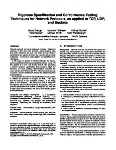
Figure 1 shows an early 4-poster vehicle test rig; the road
roughness (vertical displacement) command signal for each wheel is stored as a profile on the disk in the foreground. Digital controllers began to be introduced in the 1980’s, since when increasing real-time computing power has steadily increased the potential for implementing sophisticated control algorithms.
The control techniques used for general electrohydraulic systems have been reviewed by Edge [2,3]. General hydraulic control techniques can be applied to structural test rigs, but there are often particular features to consider too – for example stringent accuracy and bandwith requirements, command signals which may be repetitive in nature, or cross-axis interaction. A brief overview of structural test rig control methods is contained in [4], and a more detailed introduction to the simpler industrial techniques is to be found in [5]. The present paper reviews current industrial practice in hydraulic test rig control, as well as recent academic studies.
There is a substantial overlap between the control requirements for structural testing and those for dynamic materials testing. However servohydraulic materials testing machines are often simpler to control – they are typically single axis and the material
3
test specimen may have a simple characteristic.
Nevertheless load and position
accuracy requirements are high, and multi-axis materials testing machines exhibit the same sort of interactions as structural test rigs. Some components are commonly tested in materials testing frames, such as dampers and elastomeric components. Thus where relevant, materials testing machine control studies are included in this review.
Figure 2 summarises the control techniques.
PID control and well established
enhancements to tackle lightly damped plant resonance are reviewed in Section 3. Sections 4 and 5 describe repetitive and iterative control, in which the command signal can be shaped using error information from a previous trial with the same target signal. Some of these techniques are well established, others are still a matter of research. Controllers which tune themselves or adapt to plant changes in real time are discussed in Section 6. Sections 7 and 8 are chiefly concerned with multi-axis systems, and methods to improve accuracy by reducing coupling between the required control axes. Section 9 reviews some recent applications which incorporate non-linear physicallybased models into the control scheme.
Further topics related to some specific
applications are discussed in Section 10, namely the testing of part-virtual part-real specimens, and shaking table control. Shaking tables or MASTs (multi-axis simulation tables), often with 6 degrees of freedom, and are used for general purpose vibration testing, including earthquake simulation.
2
A simple model
A simple linear model of the valve, actuator and specimen dynamics is useful to have in mind in order to understand the control techniques which will be reviewed.
Figure 3 shows a single hydraulic actuator driving into a specimen consisting of mass, spring and damper. Figure 4 is a mechanical analogue of this system. The oil volumes in the cylinder are compressible and thus are represented by a spring of stiffness Ka.
4
Leakage across the piston is equivalent to a damper in series with this spring; the smaller the leakage the larger the damping constant Ca.(i.e. a larger force is required to ‘lose’ oil at the same rate). Valve flow rate q is analogous to a velocity input at the base of the damper. The transfer function from valve flow and force inputs to actuator position can be shown to be: 1 1 q f0 A Ca y M 3 C s M 2 K s Cs K s s 1 s s Ka K a Ca K a Ca Ca
(1)
where M is the total mass ( M a M s ).
The force f0 might include weight, friction forces, or cross-axis interaction. In many cases equation (1) can be approximated to:
y
1 1 q f0 A Ca Ks 1 Ka
M Cs 1 s s2 s 1 Ks Ka C a (1 / K s 1 / K a ) K s K a
(2)
Note that expanding (2) gives: 1 1 q f0 A Ca y 2 K s Cs M 3 Cs M 1 1 K s 1s s s K Ka K a Ca K a / K s 1 a Ca K a / K s 1 Ca
(3)
If Ca is large, then equation (3) is a good approximation to (1). This is true when the real pole in equation (2) (associated with leakage) is considerably slower than the pole pair associated with the resonance of the moving mass – this is almost always the case.
A more complete linear model would include the compliance of mechanical elements such as frame and load cell – Hinton [6] develops a ninth order model for a similar
5
plant. The specimen itself may also have its own internal resonances which make the mass-spring-damper model inappropriate.
The other contribution to the plant response comes from the valve dynamics. Although valve dynamics are quite often neglected in modelling studies of electrohydraulic systems, this is rarely appropriate when designing high performance controllers for structural test rigs. This is because the actuator resonant frequency in equation (2) is often similar to the valve bandwidth – it would need to be an order of magnitude lower for valve dynamics to become insignificant. A good empirical linear model of valve dynamics is a second order lag plus delay: xs
e sD 2
s s 2 1 n n
u
(4)
where xs is valve spool displacement and u is the control signal. The delay accounts for phase lag due to higher order dynamics. In a linear model, valve flow rate q is proportional to spool displacement and so may be expressed as: 1 q V ( s)u A
where
V ( s)
(5)
K v e sD / A s n
2
s 2 n
1
(6)
Thus the complete dynamic model relating control signal to actuator displacement (equations (1) and (5)) is fifth order plus a delay:
1 f0 Ca y K M 3 Cs M 2 K s Cs s s 1 s s Ka K a Ca K a Ca Ca V ( s)u
(7)
For example, Figure 5 shows a measured frequency response and a model of this type fitted to that response, for a system where both Ks and Cs are zero. Although the fit
6
appears good, there would in reality be some variation of the measured frequency response with amplitude of excitation. This is due to the well-known non-linear characteristics of hydraulic actuators (see, e.g. [7]). A key non-linearity is the variation in the valve flow gain, i.e. the ratio of spool displacement to valve flow rate, which depends on the pressure across the valve p v :
q K v xs
p v Ps
(8)
With a constant supply pressure Ps, the pressure across the valve is what remains after pressure drops across the piston (due to actuator force) and pipe work (due to flow restrictions). Another non-linearity is the variation in cylinder stiffness with piston position, which is due to changing oil volumes in the cylinder, i.e. changes in the length of the oil ‘springs’ either side of the piston. For an equal area actuator, total hydraulic stiffness varies in proportion to:
1 Ay 1 Vm
2
(9)
where y is the piston displacement from mid-stroke, A is the piston area, and Vm is the volume of oil trapped between one side of the piston and the valve when y = 0. It might be surmised that the stiffness becomes very large near the end of stroke, but due to the hydraulic cushioning volume at the end of the cylinder, and the volume trapped in the manifold, stiffness rarely changes by more than a factor of two.
Other non-linearities include:
cylinder friction (often minimised by using hydrostatic bearings, and low friction sealing arrangements)
leakage across the piston not being proportional to pressure drop (particularly when a cross-port bleed is employed)
valve slew rate limitation (maximum valve spool velocity)
7
valve overlap (valves with nominal zero-lap are usually used, but manufacturing tolerances mean that a small overlap may be present)
valve hysteresis
specimen non-linearities.
There is a clear distinction between the controller designs which are appropriate when the specimen is dominated by inertia (large M and small Ks), or by stiffness (large Ks and small M). Vibration test systems, where Ks is zero (there is no reaction frame for the specimen to transmit a force to ground) is an example of the former. Fatigue testing of metals, or some axes in a suspension test rig are examples of the latter. Referring to equation (3), if the specimen stiffness is zero then the cylinder model has a free integrator. If the moving mass is large then both resonant frequency and damping tend to be low: the challenge is to control this resonance. Where the stiffness dominates, the resonant frequency can be higher than the valve bandwidth and specific compensation for the resonance is often not required.
The variable to be controlled depends on the application.
It is often actuator
displacement or force, usually called position and load control respectively. Alternatively the controlled variable may be acceleration, force or strain at some point in the specimen, in which case it is sometimes referred to as a remote parameter.
Load control is often more problematic than position control due to zeros in the plant dynamic model. For example, if the force at point A in Figure 3 is to be controlled, the plant transfer function is: 1 ( M s s 2 C s s K s )V ( s)u f 0 Ca f M K Cs 1 1 s s s2 s 1 K a C a (1 / K s 1 / K a ) K s K a Ks Ka
8
(10)
3
3.1
Established control methods
PID control
PI (Proportional Integral) control is adequate for many test rigs. The proportional and integral gains are usually adjusted manually. The integral term is essential to provide zero steady state error. Referring to Figure 6, a good approach for tuning the integral gain is to try to cancel the single real pole in the plant model with the zero in the PI controller. This strategy is part of an auto-tuning algorithm described in [8]. The plant poles which remain are typically much faster.
Even when the specimen provides purely inertial reaction, i.e. Ks and Cs are zero, the integral term is still required. This is despite the free integrator which will now be present in the cylinder/specimen response.
As shown in Figure 6, there are
disturbances before this integrator in the forward path: d includes drift of the valve null position and valve hysteresis, and the external force f0 may include weight and cylinder friction forces. It is interesting to note the influence of the piston head seal: a better seal increases friction forces but also increases Ca (i.e. reduces leakage), and so may make little difference to the control accuracy.
The derivative term in PID (Proportional Integral Derivative) control is rarely used in structural testing applications, although common in materials testing [5]. The presence of both hydraulic and structural resonances means that the increase in closed-loop bandwidth attainable with derivative action leads, at best, to unacceptably poor robustness.
When the specimen load is dominated by inertia, the valve response dictates whether a PI controller is effective. Two cases can be envisaged:
9
1. if the valve phase lag is 90 or more at the hydraulic resonant frequency, meaning that the overall plant phase reaches -180 well before the resonance, then a PI controller may be adequate; 2. if the valve phase lag is much less than 90 at the hydraulic resonant frequency, meaning that the overall plant phase reaches -180 close to the resonance, then one of the resonance compensation techniques described in the next section will be beneficial. The example frequency response of Figure 8, described in Section 3.2.2, helps to illustrate this; it is an example of case 2. The distinction can be seen in the simulated step responses of Figure 7, which are for an 80kN actuator driving a 300kg mass. In the top trace the valve bandwidth (defined as the 90 phase lag frequency) equals the hydraulic resonant frequency, but it is higher in the other two traces. Thus when the valve bandwidth is higher than the hydraulic resonance, resonance compensation is usually required.
3.2
Compensating the hydraulic resonance
3.2.1 Cross-port bleed As stated above, in some applications, especially where the moving mass is large, a necessity for achieving acceptable bandwidth is to specifically tackle the hydraulic resonance. This is a well studied area in the hydraulic control literature over the past fifty years [2,9].
The simplest technique is to physically increase the leakage between the two cylinder chambers by introducing a cross-port bleed. This reduces Ca which increases the damping of the complex poles in equation (1). As this compensation is hydraulic rather than electronic, it does not depend on the dynamic response of the valve. However it has some disadvantages:
10
tuning usually requires manual adjustment of a restrictor mounted close to the servovalve,
flow loss can be high when exerting high loads,
it can increase the effect of unwanted forces (like friction) on the position response.
3.2.2 Common electronic resonance compensation methods Other methods involve compensating the resonance by additions to the PI controller. These alternatives are: 1. acceleration feedback, 2. differential pressure or load feedback, 3. a first order lag, 4. a notch filter.
Acceleration feedback is a well known method for increasing the damping associated with a hydraulic resonance [9]. An analysis neglecting valve dynamics would indicate that the acceleration feedback gain can be adjusted to provide any desired level of damping for the oscillatory poles. In practice, this works well as long as the hydraulic resonant frequency is much lower than the valve bandwidth. Also, the accelerometer mounting and signal conditioning should be considered carefully to ensure there are no noise issues. Any analytical approach to finding the best acceleration gain should account for the valve dynamics [9,10]. Structural test rigs with large inertial loads, such as seismic tables, are suitable for this approach. Differential pressure feedback – i.e. the pressure difference across the piston – can be used as an alternative to acceleration feedback. Clearly when the load is purely an inertial one (with no specimen forces reacted to ground) differential pressure is proportional to acceleration. Likewise if actuator force is measured, this can be used as an alternative. Differential pressure or load feedback will introduce errors due to noninertial forces – such as weight – but as long as these only change slowly the integral
11
action will compensate. When the specimen mass changes, the effect on a system with differential pressure feedback will be different from one with acceleration feedback; this difference is explored in [10].
Using a first order lag in the forward path can be effective at increasing the potential closed-loop bandwidth [8,11]. It is easy to tune manually and does not rely on a very high valve bandwidth relative to the hydraulic resonant frequency. The lag moves the 180 phase point to a frequency below the hydraulic resonance and thus improves the gain margin. Figure 8 shows an example open-loop frequency response with and without the lag. The lag time constant L can be chosen to position the -180 point at the minimum amplitude ratio before the resonance. The proportional gain Gp can then be chosen to give a desired gain margin.
An alternative to a lag is to use a notch filter. This can attenuate the resonant peak and so allow an increase in proportional gain whilst maintaining an acceptable gain margin. This method can be less robust, i.e. more susceptable to changes in the resonant frequency. This frequency will change depending of the operating position within the stroke, because the hydraulic stiffness changes as described previously (see equation (9)).
3.3
Command feedforward and Three-Variable Control
Command feedforward is sometimes used in industrial test rig controllers as a means of increasing the speed of response to the command signal. Figure 9 is a block diagram of a position controller which includes this feature.
The command derivative (i.e.
velocity) is scaled and summed with the PI control signal. Based on a very simple plant model, an integrator, the command feedforward block can be thought of as an inverse plant model, and a unity closed-loop transfer function is achieved if Gvf A Kv . The feedback controller is only required to correct for modelling errors
12
and disturbances, and the error e in the feedback loop can be interpreted as the output of a disturbance observer. In practice the errors in this simple plant model, in particular the neglected lags, mean that this form of command feedforward has limited effectiveness. Extension of the concept using non-linear models is described in Section 9.
A generalisation of some of the controller structures described previously is known as three variable control (TVC), and is shown in Figure 10. This encapsulates both acceleration feedback and command feedforward, and is often used in shaking table control, particularly for seismic testing [12]. It is a two degree of freedom controller, having the ability to independently tune the feedforward and feedback parts. There is no single well-recognised tuning method for this structure. Note that the first and second derivatives of the position feedback are required, which would usually lead to unacceptably highly sensitivity to measurement noise. In practice both position and acceleration are usually measured, and these are combined using complementary filters to estimate velocity [13,14], and all three motion variables are used in the feedback compensator.
Usually in testing applications the command signal is known before the test begins. This means that any feedforward compensation can be carried out off-line. Without the restrictions of processing time and causality, the potential for sophisticated signal processing is much greater off-line. This has allowed the development of the iterative control algorithms which are described in Section 5.
13
4
4.1
Repetitive control
Amplitude and phase control
Repetitive control is an ‘outer-loop’ technique which is applicable to cyclic waveforms. The error from one cycle is used to adjust the command to the closed loop controller for the next cycle.
Amplitude control is the most common example [5]. The amplitude of the waveform, which typically is sinusoidal, is adjusted from one cycle to the next. The outer-loop is a discrete time controller, with sample interval equal to the period of the cyclic waveform. Purely integral control is usually used, i.e.: Ri Ri 1 (Wi Yi )
(11)
where Wi is the target amplitude at cycle i, Yi is the achieved amplitude, and Ri is the amplitude of the command to the closed-loop controller. Equation (11) can be written in terms of a discrete-time transfer function: Ri
(Wi Yi ) 1 z 1
(12)
The convergence gain can be chosen manually, or adapted on-line based on the estimated ratio between command and achieved amplitudes.
The mean value of the cyclic waveform usually needs to be controlled too, and the same algorithm can be used to adjust the mean value of the command from one cycle to the next.
For multi-axis systems, with cyclic waveforms required for each axis, an additional requirement is that the achieved waveforms are synchronised, i.e. the phase relationship
14
between them is controlled. Once again, the same approach can be used to adjust the command phase so that the achieved phase matches that of the target signal. Clearly a reliable method of determining the phase of the signals is required.
An algorithm for simultaneous amplitude and phase control of sinusoidal signals is described in [15]. This estimates an inverse model of the closed-loop plant, effectively the reciprocal of the magnitude and the negated phase of the system at the test frequency, and then applies these corrections to the command signal. The magnitude and phase are in fact encoded in terms of the amplitudes two sinusoids in quadrature, as shown in Figure 11. The least mean squares (LMS) estimator [16] drives the error e(t) to zero by adjusting gains w0 and w1. The error is given by:
or
e(t ) r (t ) w0 y(t ) w1 y(t T )
(13)
e(t ) RW sin(t R ) w0 P sint R P w1 P cost R P
(14)
It can be shown that the perfect inverse model which gives e(t) = 0 is given by: w0
1 cos p and P
w1
1 sin p P
(15)
Applying the same inverse model to the target signal will adjust the gain and phase in the resulting command signal: R
1 P
and
R P
(16)
and the plant output becomes the same as the target. Note that convergence gain in the LMS estimator is normalised by the square of the signal amplitude. This corrects for the influence of signal size on convergence rate [15].
As commented in [4], the approach is only applicable to substantially linear systems, as any effect of harmonics is neglected.
However, Adaptive Harmonic Cancellation
15
(AHC) can be used to address this [4]. As the name implies, this is a frequency domain approach in which only multiples of the fundamental sinusoidal waveform frequency are considered. The amplitudes of harmonic components in the command signal are adjusted in an attempt to remove the unwanted harmonics from the output. Once this is achieved, an amplitude and phase controller can be used.
4.2
Repetitive profile control
More sophisticated algorithms, not yet widespread in the testing industry, match the entire profile of the achieved signal to that of the target. The target profile can be a complex loading profile, for example as often used for biomedical testing. Figure 12 shows an axial loading profile for a knee prosthesis wear test [17]
Shaw and Srinivasan [18] describe a repetitive controller designed in the frequency domain. The synthesis of the controller, and analysis of stability, transient response and robustness, are based on the regeneration spectrum. Results are obtained from a single-axis load-controlled electrohydraulic testing machine, showing a ten-fold reduction in error when the target is a 10Hz triangular wave.
Another application has been reported by Plummer et al [19]. In this case, due to cross-coupling, a cyclic load disturbance is experienced by an actuator exerting a side load during sinusoidal exercising of an automotive damper in a dynamic damper test rig.
In simulation a model-based discrete-time repetitive controller reduces the
disturbance by 97% after 5 cycles.
16
5
5.1
Iterative control
Overview
Iterative control is similar in concept to repetitive control, in that the command signal is adjusted from one cycle (or iteration) to the next in an attempt to achieve a target profile. In many cases the objective is to determine an effective command signal, which then only needs to be replayed once to acquire valid test data; i.e. it is not a repetitive test. In other cases, notably durability testing, the iterated command signal sequence will be replayed many times. Iterative control has become an essential tool in structural testing over the last thirty years, and is particularly prevalent in the automotive and seismic testing fields [20].
Some characteristics of iterative control are:
unlike repetitive control, each cycle starts and ends in a steady-state condition,
it can be used for multi-axis systems: controlling 4 or 6-actuators is common, and 10 or 20 is achievable,
the target signals do not have to be targets for the closed-loop controller variables – they may be targets for other sensors in the test specimen or test rig, i.e. remote parameters,
the number of target signals can be the same, greater or less than the number of axes (actuators),
a system identification phase is required before iteration can begin.
The first recorded use of iterative control was by Cryer et al in 1976 [21] for controlling a 4-post road simulator for vehicle testing. The vertical acceleration responses at the four vehicle spindles were measured on one pass of the proving ground durability route. The objective was to replicate these responses on the test rig. In order to achieve this a multi-channel frequency response from the closed-loop actuator command signals to the spindle accelerations was determined on the rig. The proving
17
ground response data were filtered by the inverse of this model to generate the actuator commands. Due to non-linearity and other modelling errors, this first set of drive signals would give errors in the responses. By passing these errors through the inverse model and adjusting the commands by the resulting correction signals, it was found, after a number of iterations of this type, that a good reproduction of the responses could be achieved. A number of commercial software packages have been developed for iterative control of structural test rigs [22 -25]. These use non-parametric frequency domain modelling as described in the next section.
The academic field of Iterative Learning Control (ILC) is concerned with similar techniques [26] but until recently has not been applied to structural testing. The origins of ILC are usually credited to Arimoto in 1984 [27]. An application to the durability testing of an automotive suspension member has recently been reported [28].
5.2
Frequency domain modelling
Conventionally, a frequency domain model of the closed-loop plant is used. The system identification stage consists of exciting the system with an m1vector rt of uncorrelated coloured noise actuator command signals. sampled to give an n1 vector yt, where n m.
The system response is
The Discrete Fourier Transforms
(DFT’s) of the signal vectors are then calculated, giving vectors R(k) and Y(k), where
k represents a set of discrete frequency values. A matrix of spectral estimates relating any two DFT vectors P(k) and Q(k) is given by: S pq ( k )
Ts T P ( k )Q * ( k ) 2
(17)
where Ts is the duration of the signals, Thus the auto and cross power spectral matrices Srr(k), Syy(k), and Syr(k) can be determined from the acquired signals.
18
The frequency domain model is the Frequency Response Function (FRF) matrix H(k), defined by: Y (k ) H(k ) R(k )
(18)
From (17) and (18), a relationship between the cross power spectrum and the input auto power spectrum can be determined: S yr (k ) H(k )S rr (k )
(19)
And so the FRF is found from: 1
H(k ) S yr (k )S rr (k )
(20)
The final stage of system identification is to check the validity of the model. One commonly used measure is the multiple coherence function. This is defined as the ratio of the predicted to measured output auto power spectra: 1 C(k ) Sˆ yy (k )S yy (k )
(21)
Using the identified model, the predicted output auto power spectrum is given by:
Sˆ yy (k ) H(k )S ry (k )
(22)
or by substituting for H(k) using equation (19): 1 Sˆ yy (k ) S yr (k )S rr (k )S ry (k )
(23)
The coherence indicates to what extent the system output behaviour is explained by the linear model driven by the known inputs. Poor coherence (substantially less than 1) can indicate poor excitation or non-linearities.
It is normal to restrict the frequency
range of model inversion to that which corresponds to high coherency, typically greater than 0.8, for each output [24].
Early implementations required the system to be square, i.e. with the same number of response channels as actuators,
so that the FRF matrix H(k) could be inverted
19
directly. Current implementations allow more target responses than actuators, in which case the following pseudo-inverse calculates the actuator commands giving the least squares best fit response: R(k ) J(k )W (k )
(24)
where the inverse model is:
J(k ) H T (k )H(k )
1
H T ( k )
(25)
and W(k) is the DFT of the target vector. Singular Value Decomposition is now being used to perform the same operation with improved numerical stability [25]. Incorporating a large number of target responses allows “global simulation”, where a reasonable match between simulation and in-service response is obtained over the entire specimen; the simulation is distributed rather than restricted to a few response locations [29]. In addition, there is scope for selecting different response channels in different frequency ranges, which can be implemented by pre-multiplying equation (18) by a frequency dependent weighting matrix giving a revised pseudo-inverse equation.
Using the inverse model, the initial test run and subsequent iterations are summarised in Figure 13. A manually adjusted gain i between 0 and 1 determines the proportion of any command signal increment which is actually used. Due to inaccuracies in modelling, implementing the full command signal may risk damaging the specimen.
Variations in current commercial iterative control packages concern the issue of adapting the plant model during the iterative process. This is desirable to ensure that linearization of what is in reality a non-linear plant occurs around the actual operating point. Thus after each iteration, the new set of actuator command signals and responses can be used to estimate a new plant model. However, as the drive signals now usually have some cross-correlation, there will be deficiencies in the model, and these can be avoided by constructing a weighted average model incorporating models from previous iterations and the original model found with uncorrelated drives. This approach was
20
first suggested by Chegolin and Konchak [30]. An alternative approach is to randomise the phase of the command signals calculated in the first iteration, and estimate a second model based on the response to these drives [25]. The final model is a weighted average of the first and second models, where the weighting depends on the coherence for each model.
5.3
Time domain modelling
Frequency domain iterative techniques are used very widely in industrial applications. However a number of time domain based techniques have been developed commercially. A key motivation has been the increase in processing speed from one iteration to the next; another is the potential for using non-linear time domain models in the future (see Section 9).
The most commercially successful time-domain approach is an extension of Adaptive Inverse Control [4, 31-34], and uses a finite impulse response (FIR) filter for the inverse plant model. It has been commercialised under the names On-Line Iteration (OLI) and Real-time Transfer function Compensation (RTC). The FIR filter length must be sufficient to capture any low frequency, lightly damped, plant dynamics, which may give a large number of coefficients, but otherwise the model is not dependent on a choice of model order.
During an identification phase the inverse model can be
calculated directly from drive and response signals using least mean squares (LMS)[16] as shown Figure 14. In the Figure, the plant plus feedback controller is represented by a FIR filter, the coefficients of which are the impulse response of the system: H ( z 1 ) z n (h0 h1 z 1 h2 z 2 ...)
(26)
Once converged, the adaptive filter is expected to be the inverse model such that:
where
G( z 1 ) z n H 1 ( z 1 )
(27)
G( z 1 ) g 0 g1 z 1 g 2 z 2 ... g m z m
(28)
21
So the overall system response is: yt z n rt
(29)
The rate of convergence of the filter during the identification phase is controlled by the LMS gain .
During iteration, the calculation of corrected command signals from the inverse model is efficient enough to be undertaken on-line, i.e. the command signal for the next iteration is ready as soon as the current iteration is finished. This is particularly convenient if drive signal correction is undertaken continuously throughout a test to compensate for changes in the properties of the specimen.
See Section 6.4 for
comments on a version of the technique for control of time-varying linear systems.
In 1993 Raath [35, 36] showed that the process could be undertaken in the time domain using a parametric model. The model used is a polynomial matrix description in the backward shift operator z-1. It is identified using least squares or a related parameter estimation method, and converted to a discrete-time state-space model for use in the iterative control algorithm. The iterative algorithm itself is similar to the frequency domain approach. As the model is parametric, an order has to be selected for each part of the multivariable model.
5.4
Closing-the-loop on the ‘remote parameters’
One research team has investigated closed loop control of the target variables, as a way of reducing the number of iterations required in automotive testing. They have used mixed sensitivity H optimisation for controller design. In [37], the target variable for one axis of a suspension test rig is actuator position, so the controller effectively just supplements the existing PI actuator position controller. Designed using an 8th order state-space model, the H controller reduces required iterations from 7 to 3.
A
position-controlled two-axis test system (vertical and lateral) at one corner of a vehicle
22
test rig is the subject of [38]. The target variables are vertical and lateral acceleration of the chassis near the wheel which is excited, so unlike the previous example, these are remote parameters. H controller design is again used to reduce the sensitivity to modelling errors and hence reduce iterations. Three controller types are considered: 1. two individual SISO controllers, which require de-tuning to remain stable in the presence of coupling; 2. a full MIMO design, requiring a 69th order model – but this is found to be too complex and impractical; 3. SISO controllers with a plant precompensator to achieve decoupling. The last approach is found to be best, with the closed-loop tracking error as low as that previously found when using the command generated by the inverse model (iteration zero). Further iterations were not undertaken.
A similar approach for controlling one axis of a four-post test rig, where axle acceleration is the target variable, is described in [39]. Iterations are reduced from 6 to 3. A notable feature is that iteration adds a correction signal to the plant input, summed with the control signal from the new closed-loop controller, and still uses the inverse plant model. As shown in Figure 15 this has implications for the effect of the iteration gain.
Generally speaking, the remote parameters are strongly influenced by the specimen dynamics, which are typically non-linear and of high order. This in the past has led to the more conservative approach of off-line iteration rather than real-time closed-loop control of these variables. Although the work described in this section has had some success, the plant modelling and choice of weighting functions is a lengthy and complex procedure, and is unlikely to form the basis of a practical industrial method.
23
6
6.1
Adaptive and self-tuning control
Self-tuning
As noted before, the characteristics of the specimen can radically alter the dynamic behaviour of the test system, and so re-tuning the controller is often required when the specimen is changed.
A self- or auto-tuning controller undergoes an automated
procedure for tuning its own gains.
A self-tuning control method for general multiaxis structural test rigs has not been developed. However, a method for single-axis systems, where the specimen force is dominated by its stiffness (such as found in materials testing), has been investigated and commericalised by Hinton [6,8].
This is a development of the PID tuning
procedure developed by Hind [40], and is applicable to controlling load, position or specimen strain. The PID compensator has the following form: s Gi u Gp d s 1e s
(30)
The proportional gain Gp and derivative time constant d are tuned using a square wave in the following way [8] 1. Increase Gp until there is significant overshoot 2. Increase d until the overshoot is a minimum. Too much d gives more overshoot again. 3. Reduce Gp until the overshoot is tolerably small (e.g. 5%).
Then the integral gain Gi is tuned using a triangle wave to give the velocity proportional to the error, barring any high frequency dynamics. The idea can be explained using a first order model. For example in load control, with the specimen modelled purely as a stiffness, and the moving mass small and hence neglected, equation (10) becomes:
24
f
where
Km u Tm s 1
1 C K 1 and K m a v Tm C a A Ks Ka
(31)
(32)
This also neglects valve dynamics. The derivative action in the PID controller can be conceived as adding some phase lead to cancel lag from higher order dynamics not included here – thus it can be neglected. If Gi is tuned so that error is proportional to velocity – or rate of change of force – then this implies that Gi Tm , giving: sf
K mG p Gi
e
(33)
So the integral-related zero cancels the plant pole.
6.2
Indirect adaptive control
The procedure described above is for one-off tuning with a new specimen, and does not accommodate changes in specimen properties during a test. Hinton has also developed an adaptive controller for adjusting controller gains in response to changes in specimen stiffness, again for materials-testing type applications [6,41]. The controller varies the proportional and integral gains initially determined by the self-tuning procedure of the previous section, in an attempt to maintain the same closed-loop transfer function. Thus, from equations (31) to (33):
and
1 1 1 1 Gi (t ) Gi (0) K s (t ) K a K s (0) K a
(34)
G p (t ) G p (0) Gi (t ) Gi (0)
(35)
The actuator stiffness is determined as part of an automated pre-tuning procedure that is carried out without a specimen. The on-line estimation of specimen stiffness uses a recursive least squares technique with a variable forgetting factor, and ensures the estimate does not drift when persistency of excitation is low. A variety of successful
25
applications have been presented, such as fatigue testing of a non-linear engine mount which exhibits a 10:1 change in stiffness within each loading cycle [41].
Lee and Srinivasan [42] have also studied indirect adaptive control for materials testing. Recursive least squares is used to identify a first order model together with a valve null offset value, i.e. three parameters, although an even simpler plant model is actually used for adaptive control implementation – just an integrator and gain. A fixed forgetting factor is used, which would cause parameter drift or ‘blow up’ when the excitation is not persistent. Pole-placement design gives a second order closed-loop transfer function, and integral action is included. For many structural test rigs, the ‘stiffness only’ specimen assumption is not valid, and the moving mass is significant so that more complex dynamics – particularly the hydraulic resonance – need to be included. A number of studies of adaptive control for this sort of servohydraulic system have been presented, although not specifically in the context of test systems (e.g. [43]).
6.3
Direct adaptive control
If the controller gains are adapted directly, rather than being calculated from plant model parameters which are estimated on-line, then the adaptive controller is of the ‘direct’ type. This is the case for the Minimal Control Synthesis (MCS) algorithm developed by Stoten [44]. This is a form of model reference adaptive controller employing an attractively simple update law. First order MCS, shown in Figure 16, has been applied to a number of test systems, and was commercialised in the testing industry under the name MIMICS [45]. Results for load control of a materials testing machine, with a stiffness-dominated specimen, are presented in [46]. The model of equation (31) should be applicable in this case, although a second order model was identified from experimental data. MCS is shown to adapt well to changes in system
26
pressure, and it is suggested that MCS would be able to adapt to specimen changes. Results for specimen changes are discussed in [47]. MCS has also been investigated for shaking table control; this is described in Section 10. MCS has mostly been demonstrated as an addition to an existing fixed-gain controller, either as an outer-loop generating a new command signal for the existing controller, or in parallel by summing the control signals from the two controllers.
However it may equally well be used
alone to control an open-loop plant. Clarke [48] compares Hinton’s adaptive controller with MCS, noting that the former uses some a priori information about the plant and so its modelling can be described as grey-box, whereas MCS is based on a black-box model. In one particular simulated example, the grey-box approach is found to be superior for adapting to stiffness changes – for which it was specifically designed – compared to MCS.
6.4
Adaptive command filtering
An alternative to adapting the compensator within the feedback loop is to manipulate the command signal using an adaptive filter. This has the advantage that as long as the adaptive filter is guarranteed stable, there is no risk of driving the closed-loop system into instability. Adaptive Inverse Control (AIC) uses a Finite Impulse Response (FIR) command filter. As described in Section 5.3, the filter is a linear approximation to the inverse of the closed-loop system, and can be used within an iterative controller to enable a set of target signals to be achieved. If the plant is in reality approximately linear, then use of the filter without iteration may allow the command to be followed quite accurately apart from a delay required for causality (Figure 14). Moreover, the LMS coefficient estimator can be used on-line to adapt the filter during the test, accommodating changes in specimen behaviour [4,34]. A MIMO adaptive filter can compensate for cross-coupling in multi-axis systems, but the rate of adaptation will reduce as the number of parameters increases. The method is unlikely to adapt quickly
27
enough to handle non-linear systems, such as those with large stiffness changes as described in Section 6.2. Only gradual changes due to specimen degradation can be addressed.
7
7.1
Motion-independent load control
Overview
Structural test rigs commonly require force to be controlled accurately in one or more directions – so called load control. Unfortunately hydraulic actuators are inherently quite stiff, and so motion of the specimen tends to cause large changes in actuator load. A closed-loop load control system will drive the actuator in response to a load error signal. For some applications, conventional PI based controllers are unable to keep the load errors sufficiently small. However, if an additional signal is available which measures or predicts the motion of the specimen, this can be used as a feedforward term to drive the actuator. Thus the actuator can be driven to match the movement of the specimen without the need for an error to be developed in the load loop. This approach can have a dramatic effect on the size of the load errors.
Two particular scenarios will be described.
In a multi-axis test rig, where one position-controlled actuator determines the motion of the specimen, and another actuator is required to accurately control the load on the specimen; a feedforward signal is passed from the former to the latter control loop.
Usually also in a multi-axis test rig, where the motion of the specimen is not entirely predictable from any actuator signal, the specimen motion is measured (using an accelerometer for example), and this measurement is used as the feedforward signal.
28
7.2
Valve cross-compensation
An example of the former scenario from automotive testing is where horizontal forces are applied in steering test rigs and in damper test rigs [19], and there is interaction from the vertical displacement i.e. the simulated road height variation. With zero specimen stiffness and damping, and low mass, the actuator model of equation (7) can be approximated by:
1 1 y V ( s)u f 0 s Ca
(36)
For example, consider the one degree-of-freedom system shown in Figure 17. This has two actuators and so is over-constrained: the actuators not only completely dictate the position of the (assumed rigid) specimen, but can also control loads applied to it. For instance, as shown in the Figure, actuator 1 may be controlled in load, and actuator 2 controlled in position. Applying equation (36) to these two actuators: f1 Ca1V (s)u1 Ca1 sy1
sy2 V ( s)u 2
(37)
1 f2 Ca 2
(38)
where f1 and f2 are the forces exerted by the actuators (tension is positive). These equations assume that the valve response V(s) is the same for each actuator – if not a pre-filter is required for one or other of the valves in order to adjust the valve dynamics so that the responses can be considered equivalent. In addition, the actuator positions and loads are linked through the specimen:
y1 ry2 and f 2 rf1 r
where
(39)
a b
(40)
Thus the plant model is:
f1 C a1 sy V ( s) 0 2
0 u1 C a1 r 1 u 2 0
29
sy2 1 / C a 2 f1 0
(41)
1 r / C a2
or
or
rCa1 f1 C V ( s) a1 1 sy2 0
1 f1 V ( s) sy 2 2 1 r C a1 / C a 2 r / C a 2
f1 V ( s) sy 2 2 1 r C a1 / C a 2
0 u1 1 u 2
rCa1 C a1 1 0
C a1 rC / C a1 a 2
0 u1 1 u 2
rCa1 u1 1 u 2
(42)
(43)
(44)
Propose the use of a ‘valve cross-compensation matrix’ to transform the control signal vector:
1 u1 u rC / C a1 a2 2
r u '1 1 u ' 2
(45)
So:
f1 C a1 V ( s ) sy 0 2
0 u '1 1 u ' 2
(46)
Thus the plant with transformed control signal is now decoupled. But in practice the following cross-compensation is commonly used:
u1 1 r u '1 u 0 1 u ' 2 2
(47)
This has the advantage that knowledge of the leakage characteristics of the actuators are not required. So:
f1 V ( s) sy 2 2 1 r C a1 / C a 2
0 C a1 u '1 rC / C 2 a1 a 2 1 r C a1 / C a 2 u ' 2
(48)
Typically, the maximum (stall) force of an actuator is reached with a few percent valve drive, i.e. the leakage is small and the value of Ca is large. Thus in equation (48) u’1 is very small compared to u’2, and it can be approximated to:
30
C a1 /(1 r 2 C a1 / C a 2 ) 0 u '1 f1 V ( s ) sy 0 1 u ' 2 2
and so approximate decoupling is achieved.
(49)
The controller shown in Figure 17
includes the valve cross-compensation of equation (47).
7.3
Variable valve cross-compensation
The valve cross-compensation term shown in Figure 17 is the velocity ratio of the actuators i.e. the velocity of the load actuator divided by that of the position actuator as dictated by the path described by the specimen. In the example, using a small angle assumption, the velocity ratio is constant. In general however, the velocity ratio may well be dependent on the position of the specimen. Figure 18 shows an example – this is one side of a steering system test rig. The ‘z’ actuator reproduces the vertical motion of the wheel hub, and the ‘x’ actuator exerts a force through a pushrod and torque arm to replicate the correct load on the track rod. To maintain a constant track rod load, as the vertical position changes, the ‘x’ actuator is required to move to compensate for the arcing of the pushrod. Using a small angle approximation, the geometric relationship is:
x
z2 2L
(50)
and thus the velocity ratio is: dx z dz dt L dt
Hence the varying valve cross-compensation term shown in the figure.
31
(51)
7.4
Feedforward of specimen motion
7.4.1 Requirement for compliance
If the motion of the specimen cannot be inferred from the drive signals of other actuators, it can be measured directly, for example using an accelerometer. Figure 19 shows an example. In this case the specimen has its own stiffness Ks, as well as a disturbance motion x2 resulting from other excitation or dynamics not shown. A compliant element, stiffness K, is inserted between the actuator and the specimen. As demonstrated below, this increases the robustness of the control system.
The force to be controlled is given by:
f K ( y x1 )
(52)
Consider a very simple actuator model: y
H u s
(53)
where u is the control signal and H is a constant. A proportional load controller will be used, with the scaled specimen velocity, found by integrating the accelerometer signal, also summed into the control signal: u G p (r f )
1 x1 Hˆ
(54)
Combining equations (52), (53) and (54): (s G p KH ) f G p KHr Kx1
where
H 1 Hˆ
(55) (56)
Clearly if is zero, i.e. the velocity feedforward gain reciprocal Hˆ is equal to H, then the load controller is completely isolated from the specimen. In practice H varies to some degree with amplitude and frequency, and so if Hˆ is chosen to be a mean value, will effectively be a varying quantity.
32
As shown in Figure 19, the specimen will have its own stiffness, and so if the mass of the x1 part of the specimen is low and can be neglected:
f K s ( x1 x 2 )
(57)
1 K s G p KH f G p KHr Kx 2 Ks
(58)
Substituting for x1 in equation (55):
Thus a necessary and sufficient condition for strict stability is:
Ks K
(59)
The lower the stiffness of the compliant element in relation to the specimen stiffness, the more robust the controller will be. Clearly the stiffness cannot be made too low, as this will require large actuator stroke and flow to achieve the required range and rate of force variations.
7.4.2 Feedforward with dynamic compensation
The simple actuator model of equation (53) implies that the actuator velocity is directly proportional to the valve control signal.
As described in Section 2, the actuator
dynamics are more complex in reality, and a fourth order linear model (perhaps with a dead time) is often a good approximation for the control signal to velocity relationship with an inertia-dominant load. Figure 20 shows the measured frequency response of an actuator used for applying loads in an automotive test rig [49]. The hydraulic resonance is clearly seen at 155Hz. Of particular interest is the phase lag of up to 25 in the 0 – 30Hz band, as this is the frequency range of interest in the application in question. Neglecting this lag will significantly impair the motion disturbance rejection performance provided by the feedforward signal. An improvement is to model the actuator response, and use an inverse model in the feedforward path, thus providing the requisite phase lead. This is shown in the block diagram of Figure 21.
33
The inverse of a fourth-order lag will be extremely sensitive to high frequency noise. Thus a low order model is required, with special attention given to moderating the high frequency magnitude of its inverse. Choosing a second-order model, with a lead term cornered at 100Hz to cancel the high frequency roll-off, then a least squares fit in the range 0-30Hz gives the following for the example shown in Figure 20:
0.562 s 2 880s 395 000 Q( s ) s 2 267 s 121 000
(60)
It can be seen that the phase and magnitude are a reasonable fit in the frequency range of interest. This and other applications are described in the next section.
Following the same derivation as in Section 7.4.1, now the actuator model is: y
1 P( s)u s
(61)
where P(s) represents the extra valve and actuator dynamics from equations (6) and (7), exemplified by Figure 20. The controller including the inverse model is:
u G p (r f )
1 x1 Q( s )
(62)
and so: (s G p KP(s)) f G p KP(s)r Kx1
where
P( s ) 1 Q( s )
(63) (64)
Thus the error caused by using a reduced-order actuator dynamic model can be quantified, given a particular motion of the specimen. However the effect on the complete system response can only be determined by including the specimen dynamics.
7.4.3 Applications of specimen motion feedforward The method was adopted in motor sport testing in the early 1990’s. In order to improve the accuracy of 4 post test rigs for racing cars, extra actuators (usually 3) were attached
34
to add vertical forces to the vehicle body to simulate aerodynamic down force and inertial roll and pitch moments. However load errors of no more than around 1% were allowable without affecting the car dynamics, which is a challenging requirement given the vigorous vertical motion of the body The use of specimen motion feedforward for this application is described in [50], and [51] contains an analysis of the likely errors. The approach is also described by Plummer as a possible way of implementing tyre models with a 7 post test rig [49,51]. The method is useful in testing aerospace systems which contain their own actuators – the loads applied by the test actuators can be made insensitive to the motion of the aircraft actuators. This is described in [52]. Compliant elements are not used here, and the stability robustness is raised as an issue, as would be expected from the analysis in Section 7.4.1.
A similar approach, described as Effective Force Testing (EFT), has been developed over the past few years for the seismic testing of large structures. Instead of placing the structure on a shaking table, the base motion is zero, and a horizontal actuator is attached to each mass concentration.
Pre-calculated inertial forces (mass times
simulated ground acceleration) are applied by each actuator, and the resulting relative motion of the structure is the same as if ground excitation had been used [53]. Initially it was found that the force error with conventional load control was too great for this application, particularly for lightly damped structures near resonance.
A velocity
feedforward approach was first described by Dimig et al [54]. The method has been enhanced by including a phase advance network, equivalent to the inverse model of Section 7.4.2, and this is shown by Shield et al [53] to give very good results. However no mechanical compliance is built into the system, and consequently the velocity gain has to be slightly conservative.
Load-controlled testing of structures in civil engineering is also address by Reinhorn et al [55]. Specimen motion feedforward is adopted, with the following features:
35
mechanical compliance (a coil spring) is included;
specimen position is measured, and fed forward through an inverse actuator model
an inner actuator position control loop is used;
load control is open loop – i.e. position control, with the known stiffness of the coil spring, is utilised.
Using an actuator position inner loop gives the benefit of reducing the sensitivity to changes in actuator dynamics (for example due to oil temperature changes).
A
disadvantage however is that using specimen position, rather than measuring velocity or acceleration, will give greater measurement noise sensitivity.
8
8.1
Kinematic transformation
Transforming to specimen co-ordinates
In multi-axis test rigs, design constraints often mean that the physical arrangement of actuators does not give the most meaningful control axes with regard to the specimen. For example, consider the two axis suspension test rig shown in Figure 22. The actuators control the vertical displacement at two points on the dummy wheel. The two degrees of freedom which are meaningful with regard to the specimen are bounce (z) and caster (); these will be called specimen co-ordinates.
Using small angle
approximations, bounce and caster can be deduced from the measured actuator displacements thus:
where
y1 z P y 2
(65)
0.5 0.5 P 1 / a 1 / a
(66)
As shown in the figure, closed-loop control of bounce and caster can be achieved using these derived measurements as feedbacks. An inverse transformation is required to
36
convert the control signals back from specimen to actuator co-ordinates. In principle the inverse transformation would be:
where
P 1 UV
(67)
0 1 1 1 . U and V 1 1 0 a / 2
(68)
but in practice the diagonal matrix V is often subsumed into the PI controller, leaving U as the inverse transform as shown in Figure 22.
The general case of a multi-axis rig controller with PI position controllers in specimen co-ordinates is shown in Figure 23. The same principle may be used for achieving load control in specimen co-ordinates, or a mixture of load and position control axes may be required. An example is the mixed load and position control of opposing actuators in a cruciform materials testing machine [56].
In cases where accuracy is paramount, the approximations which lead to a fixed matrix (i.e. linear) transformation are not acceptable. Instead the trigonometrical equations which fully describe the geometry of the actuator configuration should be used. For example, if a third actuator is attached to the suspension test rig of Figure 22 at point X, orientated horizontally, then the planar motion of the dummy wheel is fully determined. The specimen co-ordinate vector is a function of the three actuator displacements:
where
y s f (y a )
(69)
x y1 y s z and y a y2 y3
(70)
In order to determine the inverse, the transformation first needs to be linearized about the current operating position by a small perturbation analysis. The resulting Jacobian, a 3x3 gradient matrix, is defined as: J (y a )
37
y s y a
(71)
The inverse transform is then given by J 1 (y a ) .
A full six degree-of-freedom suspension test rig, or similar six axis systems such as shaker tables, can be treated in the same way.
For parallel mechanisms of this type,
there is no closed-form solution to the forward kinematic calculation. However a realtime numerical solution is quite feasible with current processing power.
Note that many test systems are still designed with nominally orthogonal actuators, and thus a very simple linear transformation exists at zero position. As actuator strokes are relatively small, rarely more than +/-10% of the distance between joints, this transformation is a reasonable approximation over the full working range. If iterative control is to be used to achieve target accelerations or loads, the geometric nonlinearity can be neglected as it will not be large enough to disrupt the iteration process. However there is an increasing desire, and a necessity in some applications, for accurate control without iteration. More alternative mechanical arrangements are also being used, such as Stewart platforms, where the kinematic transformation is not so simple and a fixed matrix may be too inaccurate.
8.2
Modal control
Modal control refers to controlling the resonant modes of a plant individually, and requires a co-ordinate transformation which decouples those modes [11]. For example, consider a six degree-of-freedom shaker table with a rigid specimen. The table plus specimen inertia will interact with the actuator oil column compliance to give six rigid body modes of vibration.
From equation (7), if damping is neglected, a linear single axis model for an actuator i with an inertial load is given by:
38
( Ms 2 K a ) yi K a
V ( s) ui s
(72)
A multi-input multi-output linearized model for a six axis system is [11]: V ( s) s 2 y a M 1 K a y a ua 0 s
(73)
where M and Ka are 6x6 mass and stiffness matrices. This assumes that all the valves have the same dynamics, so the scalar valve model V(s) can be retained. A co-ordinate transformation will be applied as shown previously in Figure 23, giving the following plant dynamics in the transformed co-ordinates: V ( s) s 2 y s PM 1 K a P 1 y s us 0 s
For modal control, matrix P is chosen to diagonalize P-1M-1KaP.
(74) For example, if P
has as its columns the eigenvectors of M-1Ka, and the eigenvectors are linearly independent so that P is non-singular, then this diagonalization is achieved, and: 1 2 1 1 P M KaP 0
2
2
0 2 6
(75)
Each i2 term is the square of the natural frequency of one mode; these are the eigenvalues of M-1Ka.
The co-ordinate transformation has decoupled the modes,
allowing individual control loops to be designed for each of the transformed axes.
True modal control is very rarely used in practice, as it requires accurate identification of mass and stiffness properties. A special case is where there is a single ‘centre of stiffness’ point (i.e. the centre of rotation when a pure moment is applied to the mass), and this coincides with the centre of mass, then a co-ordinate transformation to this point of the type described in the previous section also achieves modal decoupling. In practice a central point in the test system, such as the centre of the top surface on a shaker table, is often chosen for the co-ordinate transformation, as this very roughly approximates to the centres of stiffness and mass, and so gives a degree of decoupling.
39
This decoupling is why the approach described is preferable to doing a transformation from specimen to actuator co-ordinates on the command signal, and closing the loops on individual actuators, as has sometimes been done in the past [57].
9
Non-linear control
A number of systems have been built with controllers based on non-linear physical models of the plant. Some of these controllers are open loop; others include feedback. They all incorporate some form of inverse non-linear model. The systems described in published literature are all for impact or shock testing of some kind, where velocity or acceleration has to be controller accurately over a short duration (of the order of 10ms to 100ms). Only inertial parameters for the specimens need to be ascertained for these systems; a physical modelling approach is not so feasible for test rigs in which each new specimen has its own complex set of dynamics.
A high strain rate materials testing application is described in [58]. Velocity has to be kept constant in the face of an a priori unknown impact load. Iterative control is used, where the time-domain inverse model is derived from physical modelling. A static non-linear velocity gain curve is used, and the actuator dynamic model is linearised about the target velocity – this has a significant effect on the damping. Similarly, openloop control with iteration is used to achieve a desired acceleration profile for the 2.5MN vehicle crash testing catapult described in [59]. The physical equations are rearranged to obtain a detailed non-linear inverse model. Iteration involves adding the acceleration error signal to the previous target signal and passing this through the inverse model. Using the perturbed target signal rather than the error signal as the inverse model input maintains the correct operating point, as clearly superposition is not valid for non-linear models.
40
A large shock testing system is described in [60], and the controller is represented by Figure 24a. The inverse plant model Bˆ 1 is in the command feed forward path, and there is a conventional feedback controller as well. Note that there is no feedback control action if the inverse plant model is exact, so the feedback path can be considered as a disturbance observer.
There would be an advantage in including the inverse model in the forward path of the feedback loop, thus greatly simplifying the feedback compensator.
However the
inverse model includes high order differentiation, which is only feasible where the frequency range of the signal passing through the model is well controlled, which can be the case with a command signal. High order unmodelled plant dynamics and measurement noise would give serious problems with the inverse model in the feedback loop. Nevertheless, for the impact velocity control system described in [61], the plant model is partitioned into a non-linear cylinder model C and a linear valve model V(s), arranged as shown in Figure 24b. Using both position and acceleration feedback the inverse cylinder model in the feedback loop is found to be feasible, and as the remaining valve dynamics are ‘well behaved’ – in particular well damped – a simple proportional feedback compensator is effective.
10 Comments on two specific applications
10.1 Model-in-the-loop testing
Model-in-the-Loop (MiL) testing, real-time substructuring, or real-time hybrid testing, are all terms used for a relatively new concept in which the test specimen is part real and part virtual. The virtual part is implemented via a real-time computer simulation. This arrangement has a number of potential advantages depending on the application, e.g.:
41
only the key component with unknown dynamics need be physically tested, reducing the cost, complexity and size of the physical test apparatus;
a newly designed system can be tested even if some parts have yet to be physically realised – these parts are simulated instead;
sometimes it is difficult to physically replicate in-service conditions in the laboratory, e.g. temperature effects or aerodynamic forces, and so the affected systems can be represented more accurately by a computer model;
the characteristics of the simulated system can be varied to represent alternative configurations – this is more convenient than changing physical components.
Hardware-in-the-loop (HiL) simulations have been used successfully for a number of years. The model-in-the-loop concept differs in that the interface between real and virtual parts is a mechanical one requiring actuators and sensors which would not have otherwise been present; these actuators and sensors have there own characteristics which detract from the realism of the complete system response.
Figure 25 shows the principle of MiL testing: the complete test specimen consists of a numerical model interacting with a physical system. The interface sensors and actuators not only have their own dynamic characteristics, but they are affected by noise and disturbances, and the actuator response is dependent on the behaviour of the attached physical system (shown by the dashed line). The feasibility of including aerodynamic and tyre models in “7-post” Formula One car test rigs is analysed in [51]; a general framework for MiL testing is also developed. However the concept has been most widely explored in the civil engineering field [62], where it has evolved from pseudo-dynamic testing (PsD) [57]. PsD involves calculating structural displacements from a numerical model, imparting these quasi-statically to a physical structure, and then feeding measured forces back to the model. Any timedependent specimen behaviour, such as damping, is lost, and so real-time MiL testing may be preferrable. However, difficulties associated with limited actuator response in
42
have been a major concern for real-time testing. Horiuchi et al [63] were the first to propose a command filter for compensating the limited response of the positioncontrolled actuator. A time delay was used as a simple model of the closed-loop actuator, which was compensated by a moving average filter of order n; for example using n = 3, the proposed filter was: 4 6 z 1 4 z 2 z 3
(76)
The actuator delay is one sample interval. This design is justified on the basis of extrapolating a polynomial fit to the current and previous actuator output samples. The frequency response of this filter is shown in Figure 26. In [64], Darby et al noted that the actuator delay varied with the stiffness of the physical system, i.e. the actuator response is dependent on physical specimen dynamics. The delay was estimated during a test thus allowing adaptive delay compensation. The need to estimate the delay online is also noted in [65], and a new command modification is proposed in which the command is filtered by first and second order high pass filters and then summed with the original signal. This modification is justified by a crude stability analysis, and in general is no improvement over the established method.
Although the simplicity of the delay compensation approach is attractive, the consequences of both the closed-loop actuator and the compensation deviating from the delay and negative delay (respectively) assumptions has not been fully analysed. An alternative approach to ‘delay compensation’ is to force the closed-loop actuator response to follow a fixed reference model, and then cancel the reference model dynamics. To achieve this, Lim et al [66] have used a form of the adaptive minimal control synthesis (MCS) algorithm for the actuator control loop, giving a consistent actuator response; low frequency experimental results are presented. Alternatively the entire numerical model can be used for the MCS reference model [67]. However, difficulties have been encountered when the numerical model is of higher order than the reference model usually used in MCS, which is of order one [68]. Partitioning the
43
numerical model to allow the reference model to be first order has proved to be a successful way of tackling this problem [68].
10.2 Shaking tables for seismic testing
Motion control of large multi-degree of freedom seismic testing tables has been studied by a number of researchers, particularly in Japan. This has been motivated by the Japanese government’s investment in large-scale testing facilities following the Hanshin-Awaji earthquake at Kobe in 1995 [69]. Although iterative control is often used to obtain the required base accelerations, some tests involve the failure or partial failure of the specimen, and thus iteration cannot be used. Hence improvements in closed-loop control have been sought.
A particular problem is that the mass of table plus specimen is usually large, and so the hydraulic resonance is low. Four European tables are reviewed in [70], with sizes between 3m and 5.6m square; the hydraulic resonances are mostly in the range 10 to 50Hz depending on axis and specimen. Real earthquake signals do not have significant frequency content above 8Hz [70], but the frequency must be scaled up when reducedscale model buildings are tested, and many such shaking tables are designed to test up to 100Hz. The E-defense shaking table which has a 1200 tonne capacity, and is capable of testing many buildings at full-scale, has a specified bandwidth of 15Hz, but calculated hydraulic resonances in the range 3.1Hz to 8.3Hz [69].
Thus the
requirement is to achieve acceptable motion tracking in a frequency range extending well beyond the hydraulic resonances. Although this has been achieved with iteration, it is still an open issue when iteration cannot be used.
PI control with acceleration or differential pressure feedback has often been used for this application in the past (see Section 3.2). However, Three-Variable Control is now becoming more common, increasing flexibility and providing command feedforward to
44
improve the bandwidth.
In current practice, tuning the controller depends on the
expertise of the operator; however a model-based pole-placement tuning method is described in [12]
Loops are commonly closed on the table degrees-of-freedom, as an approximation to the modal control described in Section 8.2. Kinematic transformation either uses a full geometric model or a linear approximation.
Most six degree-of-freedom seismic
shaking tables are over constrained, i.e. they possess more than six actuators (so as to spread the load more evenly on the table structure) [70]. So, for example, a typical 8actuator table would have an additional two ‘modal’ loops controlling the shear and twist deformations of the table. These would ideally be load or differential pressure control loops which are commanded to zero. If they are position control loops then shear and twist loads are still likely to be experienced by the table due to geometric or position measurement errors.
Adaptive control has been studied for shaking tables, which has the attractive potential of adapting to new specimens or changes within an existing specimen during testing. Trials with first order MCS (Minimal Control Synthesis) are described by Stoten and Gomez [71] for two shaking tables. First order MCS provides adaptive tuning of gains in a proportional or PI controller, and can be used alone, or (as for the results shown) in conjunction with an existing fixed gain controller. Tests include 1Hz or 2Hz sinusoidal commands, and earthquake signals with frequency content up to around 6Hz. MCS is compared with detuned fixed gain controllers of low bandwidth (–3dB frequency of 1Hz to 2Hz), and shows some promise as an alternative to manual PI tuning. Similarly, some improvement in tracking response is demonstrated using MCS compared to a fixed controller in [72], where both one and two-axis control of a 40 tonne table with a 41 tonne flexible specimen are described. The fixed controller is detuned to ensure stability robustness in the presence of parameter variation due to specimen changes. Tests include a 2 to 3.5Hz synthetic earthquake signal, and a frequency response test where small improvements in the 3Hz to 7Hz range are
45
evident. The two adaptive weights and the reference model time constant are different for the two axes, implying that there is some sensitivity to these parameters; if there is a need to ‘tune’ the algorithm then MCS does not offer an advantage over manual PI tuning. Additional tests are required at higher frequencies to investigate the behaviour of the algorithm (based on a first order model) when higher order dynamics – particularly the hydraulic resonances – are excited.
A novel approach to reducing the influence of the specimen on the table response is introduced in [73]. Mirroring the approach described in Section 7.4, where specimen motion is measured and fed forward to cancel motion disturbance in a load loop, here specimen force is measured and fed forward to cancel force disturbance on a position loop. The full derivation is contained in [74], where a third-order lead term is used in the force feedforward signal as an approximate inverse of the transfer function from valve drive to specimen force. Results are shown for a flexible 600kg specimen mounted on a small shaking table, and the disturbance due to specimen resonance at either 3.8 Hz or 6.8Hz (depending on specimen configuration) is much reduced. It is probable, however, that the amplification of force measurement noise could sometimes be a difficulty with this technique.
11 Conclusions
The use of an appropriate control method is essential in order to maximise the effectiveness of any dynamic test system. In many instances, a simple ProportionalIntegral (PI) control provides the best balance between performance, robustness and tuning simplicity. In many other instances this is not the case, and more advanced techniques which modify either the feedback loop or shape the command signal are in common usage.
46
Structural test systems with many interacting actuators and with non-linear, high order dynamics, provide a significant challenge to the control engineer. The use of ‘outer loop’ methods to shape the command signal based on previous cycles or trials has proved remarkably successful in achieving accurate control without the need for extensive optimisation of the feedback controller. These methods rely on the ability to repeat a target waveform which is known a priori, and range from simple amplitude adjustments for a sinusoidal waveform, to frequency-domain based iterative control. The algorithms have mostly been developed for automotive testing, but subsequently adopted in other industries. Iterative or repetitive control is not yet common place in biomedical testing, but this is likely to be a future development. Despite the success of ‘outer loop’ methods, there are a number of drivers for improving feedback controller design:
Iterative control relies on repeatability: accuracy is reduced if the test specimen degrades significantly during testing.
An expert operator is required to adjust gains and other parameters during the iteration process for multi-axis non-linear rigs – better feedback control can linearize the plant and improve coherence.
Eradicating the need for any iteration in simpler systems improves usability.
The target signal is not always known beforehand, such as for model-in-theloop testing applications.
Perhaps the most promising approaches for improving closed loop controller design have been based on knowledge of the physical test system. These include adaptive control for varying specimen stiffness, and inverse physical models for improved motion control of inertial loads. However, more generally, the test specimen dynamics are more complex and less certain, so it is not clear that such techniques can be applied more widely.
47
Testing in many industries could benefit by adopting the model-in-the-loop approach, and this is likely to be a major driver for improving actuator speed of response, which would include control as well as hardware optimisation.
For example, the
improvement in load control through specimen motion feedforward, which model-inthe-loop testing has already motivated, is likely to be developed further in the future.
Acknowledgements The author wishes to acknowledge contributions over a number of years, upon which this paper is in part based, from colleagues at Instron Ltd and IST Gmbh, in particular John McAllister, Gerald Jung, and Glen Wardrop, and also from Colin Dodds of Dodds and Associates.
48
References
1. Olley, M. Chassis Design: Principles and Analysis.
Eds. W.F.Milliken,
D.L.Milliken. Professional Engineering Publishing, London, 2002. 2. Edge, K.A. The control of fluid power systems – responding to the challenges. Proc Instn Mech Engrs,Vol 211 Part I, 1996, 91-110. 3. Edge, K.A., On the control of electrohydraulic systems – some recent research contributions. The Eighth International Conference on Fluid Power, SICFP’03, Tampere, Finland, May 2003. 4. Soderling, S., Sharp, M., Leser, C.
Servo controller compensation methods:
selection of the correct technique for test applications. SAE International, paper 1999-01-3000, Warrendale, USA, 1999. 5. Hinton, C.E., Dynamic Control Models. In. Materials, metrology and standards for structural performance. Eds: B.F.Dyson, M.S.Loveday, M.G.Gee. Chapman and Hall, London, 1995. 6. Hinton, C.E., Control of servo-hydraulic materials-testing machines. DPhil Thesis, University of Oxford, 1992. 7. McCloy, D, Martin H R, Control of Fluid Power: Analysis and Design. Pub: Ellis Horwood, Chichester, 1980. 8. Hinton, C.E. The maximum gain, minimum-integral principle applied to materials testing. IEE Colloquium – Getting the best out of PID in machinery control, London, October 1996. 9. Bell, R., de Pennington, A.
Active compensation of lightly damped
electrohydraulic cylinder drives using derivative signals. Proc Instn Mech Engrs, Vol 184 Pt 1(4), 1969-70, p83-98. 10. Plummer, A R A new acceleration feedback design method for electrohydraulic motion control systems. PTMC 2006, Bath, September 2006. 11. Plummer, A.R., Modal control for a class of multi-axis vibration table. Control 2004, Bath, UK, Sept 2004.
49
12. Kajiwara, K., Sato, E., Mitsuta, T., Watanabe, S., Tagawa, Y. and Takai, S., Design methodology of the three-variable control method for shaking-table control with acceleration feedback, Proc Fourth Symp. on Enhancement of Earthquake Performance of Infrastructures Based on Investigation into the Fracturing Process, Tokyo, pp.53-58, (in Japanese), 2003. 13. Stoten, D.P., Fusion of kinetic data using composite filters. Proc. Instn. Mech. Engrs, Part I, Journal of Systems and Control Engineering, 2001, 215, 483-497. 14. Plummer , A.R. Optimal complementary filters and their application in motion measurement. Proc. Instn. Mech. Engrs, Part I, Journal of Systems and Control Engineering, Accepted. 15. US Patent 5,124,626. Sinusoidal amplitude and phase control for an adaptive feedback control system. June 1992. 16. Elliot, S.J., Signal Processing for Active Control. Academic Press, London, 2001. 17. ISO standard 14243-1. Implants for surgery – Wear of total knee-joint prostheses. ISO, Geneva, 2002. 18. Shaw, F-R., Srinivasan, K. Discrete-time repetitive control system design using the regeneration spectrum. American Control Conference, Boston, 1991. 19. Plummer, A R, Hatonen, J J, Owens, D.H. Using repetitive control to eliminate disturbances in damper test rigs. IFAC World Congress, Prague, July 2005. 20. Dodds, C J, Plummer A R Laboratory road simulation for full vehicle testing – A Review. Symposium on International Automotive Technology, Pune, India, January 2001, 487-494. (SAE 2001-01-0047). 21. Cryer, B.W., Nawrocki,- P.E. and Lund, R.A. Road simulation system for heavy duty vehicles, SAE Paper No. 760361, Warrendale, USA, 1976. 22. Dodds. C.J. A computer system for multi-channel remote parameter control of a test specimen, MTS publication, Minnesota, 1977. 23. Craig, J. ITFC - How it works and where to use it, Schenck publication, Darmstadt, 1979.
50
24. Craig, J. Iterative transfer function compensation using a time-domain and a frequency domain approach. EIS Conference on Progress in Computer Modelling and Laboratory Testing, Stratford-upon-Avon, UK, October 1993. 25. De Cuyper, J., Coppens, D., Liefooghe C., Debille J
Advanced system
identification methods for improved service load simulation on multi-axial test rigs, European Journal of Mech. & Env. Eng. M, Vol.44 (1), 27-39, 1999. 26. Owens, D.H., Hatonen, J. Iterative learning control – an optimization paradigm. Annual Reviews in Control 29, 2005, 57-70. 27. Arimoto, S., Kawamura, S., Miyazaki, F.
Bettering operation of robots by
learning. Journal of Robotic Systems, 1, 1984, 123-140. 28. Daley, S., Hatonen, J., Owens, D. Hydraulic servo system command shaping using iterative learning control. Control 2004, Bath, UK, Sept 2004 29. Fletcher, J.N. “Global simulation: new technique for multiaxis test control”, Sound and Vibration, November 1990, 26-33. 30. Chegolin, P.M. and Konchak, V.S. “Control of an automobile test stand on a full spectral matrix”, Institute of Engineering Cybernetics, USSR, 1982. 31. Widrow, B, Walach, E Adaptive Inverse Control. Prentice Hall, New Jersey, 1996. 32. US patent 5,394,071. Control network with on-line iteration and adaptive filter. Feb 1995. 33. US patent 5,623,402. Multi-channel inverse control using adaptive finite impulse response filters. April 1997. 34. Grote, P, “Adaptive control techniques for component testing”, Symposium on Indian Automotive Technology, 339-347, 1994. 35. Raath, A. D., “ Service load simulation testing in the time domain”, Environmental Engineering, September 1993, 8-15. 36. Raath, A. D., “Structural dynamic response reconstruction in the time domain” PhD Thesis, University of Pretoria, 1992. 37. De Cuyper, J., Vaes, D., Dehandschutter, W., Swevers, J., Verhaegen, M., Sas, P.
Experimental H control to improve an industrial off-line tracking control
51
scheme on an automotive suspension test rig Conference on Control Applications, CCA02-INV5306, 2002. 38. Vaes, D., Swevers, J., Sas, P. Experimental validation of different MIMOfeedback controller design methods. Control Engineering Practice 13 (2005) 14391451. 39. De Cuyper, J., Verhaegen, M., Swevers, J.
Off-line feedforward and H
feedback control for improved tracking on an industrial vibration test rig. Control Engineering Practice 11(2), February 2003, Pages 129-140 40. Hind, E.C. Manual Tuning of Controllers using set point changes. Trans Inst Measurement and Control, Vol 3, No. 3, 1981. 41. Clarke, D.W., Hinton, C.J., Adaptive control of materials testing machines. Automatica, Vol 33, No. 6, 1119-1131, 1997. 42. Lee, S.R., Srinivasan, K.
Self-tuning control application to closed-loop
servohydraulic material testing. ASME Journal of Dynamic Systems Measurement and Control, Vol 112, 1990, 680-689. 43. Plummer, A.R., Vaughan, N.D. Robust adaptive control for hydraulic servosystems. ASME Journal of Dynamic Systems Measurement and Control, June 1996, 237-244 44. Stoten, D.P., Benchoubane, H. Robustness of a minimal control synthesis algorithm. Int J Control, 1990, 51, 851-861. 45. Stoten, D.P., Johnson, C. Minimal control synthesis for servo-hydraulic systems. EIS Conference: Embracing Test, Development and Analysis, Gaydon (UK), October 1998. 46. Stoten, D.P. Implementation of minimal control synthesis on a servo-hydraulic testing machine. Proc IMechE, Vol 206, 189-194, 1992. 47. Bulut,S. The robustness of reduced order minimal controller synthesis control in the plastic region. Proc IMechE Part I, Vol 214, 185-195, 2000. 48. Clarke D.W. Adaptive control of servohydraulic materials testing machines: a comparison between black- and grey-box models. In Proc IFAC workshop on Adaptive Control and Signal Processing, Glasgow, 1998.
52
49. Plummer, A R A servohydraulic control system for implementing virtual components in mechanical systems PTMC 2003, Bath, September 2003, 131-146.. 50. Blows, F
Race track simulation with aerodynamic loading
EIS Conference,
Advances in Computer Modelling Techniques and Laboratory Testing, Gaydon, UK, October 1999. 51. Plummer, A R Model-in-the-loop testing. Proc IMechE Vol 220 Part I, 183-199, 2006. 52. Jacazio, G., Balossini, G A high performance force control system for dynamic loading of fast moving actuators. PTMC 2005, Bath, September 2005, 3-15. 53. Shield, C.K., French, C.W., Timm, J. Development and implementation of the effective force testing method for seismic simulation of large-scale structures Phil Trans R Soc Lond A (2001) 359, 1911-1929. 54. Dimig, J, Shield, C, French, C, Bailey, F Clark, A Effecting force testing: a method of seismic simulation for structural testing. J. Struct. Engng 125, 10281037. 55. Reinhorn, A.M., Sivaselvan ,M. V., Liang, Z., Shao, X
Real-time dynamic
13th World Conference on Earthquake
hybrid testing of structural systems Engineering, Vancouver, August 2004.
56. McAllister,J.M. The control of cruciform testing systems using opposed pairs of servohydraulic actuators.
Seventh Bath International Fluid Power Workshop.
Bath, UK, September 1994, 311-320. 57. Williams, M.S., Blakeborough, A. Laboratory testing of structures under dynamic loads: an introductory review Phil Trans R Soc Lond A (2001) 359, 1651-1669. 58. Plummer, A R Iterative velocity control for a high speed hydraulic actuator. PTMC 2001, Bath, September 2001, 339-354. 59. Plummer, A R Iterative acceleration control of a hydraulic actuator for vehicle crash simulation PTMC 2002, Bath, September 2002, 191-202. 60. Krantz, D, Hessburg, T. Feedforward control (based on model inversion) and system performance prediction using high-fidelity nonlinear dynamic hydraulic
53
system modeling. Proceedings of the IEEE International Conference on Control Applications, Oct 5-7 1997, Hartford, CT, USA, 57-62. 61. Plummer, A.R. Closed-loop velocity control for an electrohydraulic impact test system PTMC 2005 Bath, September 2005, 75-90. 62. Blakeborough, A, Williams, M.S., Darby, A.P., Williams, D.M.
The
development of real-time substructure testing Phil Trans R Soc Lond A (2001) 359, 1869-1891. 63. Horiuchi, T., Inoue, M., Konno, T., Namita, Y. Real-time hybrid experimental system with real-time actuator delay compensation and its application to a piping system with energy absorber. Earthquake Engng. Struct. Dyn., 1999, 28, 11211141 64. Darby, A.P., Williams, M.S., Blakeborough, A. Stability and delay compensation for real-time substructure testing.
Journal of Engineering Mechanics, December
2002, 1276-1284. 65. Horiuchi, T., Konno, T. A new method for compensating actuator delay in realtime hybrid experiments. Phil Trans R Soc Lond A (2001) 359, 1893-1909. 66. Lim, C.N., Neild, S.A., Stoten, D.P., and Drury D., Real-time dynamic substructure testing via an adaptive control strategy. First International Conference on Advances in Experimental Structural Engineering, Nagoya, Japan, July 2005, 393-400. 67. Wagg, D.J., Stoten, D.P. Substructuring of dynamical systems via the adaptive minimal control synthesis algorithm
Earthquake Engineering and Structural
Dynamics, vol 30, 865-877, 2001. 68. Neild, S.A., Drury, D., and Stoten, D.P. An improved substructuring control strategy based on the adaptive minimal control synthesis algorithm. Proc IMechE, Part I, Journal of Systems and Control Engineering, 2005, 219, 305-317. 69. Ogawa, N., Ohtani, K., Katayama, T. and Shibata H., Construction of a threedimensional, large-scale shaking-table and development of core technology, Phil. Trans. R. Soc. Lond. A, 359, pp1725-1751, 2001.
54
70. Crewe, A.J., Severn, R.T., The European collaborative programme on evaluating the performance of shaking tables. Phil Trans R Soc Lond A (2001) 359, 16711696. 71. Stoten, D. P. and Gomez, E., Real-time adaptive control of shaking tables using the minimal control synthesis algorithm, Phil Trans R Soc Lond A, 359, pp16971723, 2001. 72. Shinohara, Y. and Shimizu, N. and Sato, E.,
Experimental study on shaking-
table control using adaptive control, Proc. American Soc. of Mech. Eng., Pressure Vessel and Piping Conference, Seismic Engineering, San Diego (CA), USA, pp.209-216, 2004. 73. Horiuchi, T, Dozono, Y, Konno, T
Improvement of accuracy of seismic
acceleration waveforms of shaking tables by compensating for the reaction force in real time. Transactions, SmiRT16, Washington, August 2001. 74. Iwasaki, M, Ito, K, Kawafuku, M, Hirai, H, Dozono, Y, Kuosaki, K. Disturbance observer based practical control of shaking tables with non-linear specimen. 16th IFAC World Congress, Prague, July 2005.
55
Notation
a
Lever arm length
A
Piston face area
b
Lever arm length
Ca or Cai
Internal cylinder damping
Cs
Specimen damping
C(k)
Multiple coherence function
D
Valve model dead time
e or e(t)
Control loop error signal
f , f1 or f2
Force on specimen
f0
External force on piston
g0 … gm
Coefficients in G(z-1)
Ga
Acceleration feedback gain
Gi or Gi(t)
Integral gain
Gp or Gp(t)
Proportional gain
Gv
Velocity feedback gain
Gaf
Acceleration feedforward gain
Gpf
Position feedforward gain
Gv
Velocity feedforward gain
G(z-1)
Finite impulse response inverse plant model
H
Gain of plant modelled as an integrator
Hˆ
Estimate of plant model gain
H(k)
Frequency response function matrix
H(z-1)
Discrete-time plant model
i
Integer
J(k)
Inverse frequency response function matrix
J(ya)
Jacobian matrix
56
K
Stiffness of compliant element
Ka
Cylinder oil stiffness
Ka
Cylinder oil stiffness matrix
Ks or Ks(t)
Specimen stiffness
Km
Gain in first order plant force model
Kv
Valve flow gain
L
Pushrod length
M
Combined specimen and piston mass
Ma
Piston mass
M
Mass matrix
Ms
Specimen mass
pv
Pressure drop across valve orifices (total)
P
Co-ordinate transformation matrix
P
Plant amplitude ratio
Ps
Supply pressure
P(s)
Plant model, excluding integrator
q
Volume flow rate of oil
Q(s)
Low order estimate of plant model P(s)
r , r(t) or rt
Command signal
R
Command filter amplitude ratio
Ri
Command signal amplitude
R(k)
Discrete fourier transform of command signal
s
Differential operator
Srr(k)
Command auto power spectral matrix
Syr(k) & Sry(k Cross power spectral matrices Syy(k)
Response auto power spectral matrix
Sˆ yy(k)
Predicted response auto power spectral matrix
t
Time
T
Time delay
57
Tm
Time constant in first order plant force model
Ts
Signal duration
u or ui
Control signal
u’
Control signal passed to an inner loop
u’i
Control signal before a linear transformation
U
Factor of inverse of transformation matrix P
V
Factor of inverse of transformation matrix P
V(s)
Valve dynamics model
Vm
Mid-stroke oil volume between piston and valve (one side only)
w0
Adaptive inverse control weight
w1
Adaptive inverse control weight
w(t)
Target signal
W or Wi
Target signal amplitude
x
Horizontal actuator position
xs
Valve spool position
xi
Displacement of parts of a specimen
y or yi
Piston position
y(t) or yt
Response (plant output) signal
Yi
Response (plant output) signal amplitude
ya
Displacement in actuator co-ordinates
ys
Displacement in specimen co-ordinates
Y(k)
Discrete fourier transform of output signal
z
Vertical actuator position
z-1
Backward shift operator
Iteration gain, convergence gain, or MCS adaptation gain
MCS adaptation gain
Normalised additive plant model error
Phase
58
L
Lag time constant
d
Derivative time constant
Frequency
k
One of a set of discrete frequency values
i
Modal frequencies
n
Valve natural frequency
Valve damping ratio
59
Figure 1 Early 4-post rig with control system
60
Closed loop compensation
Command shaping – non-real time
PID +First order lag +Notch filter +Pressure f/b +Acceleration f/b
Three variable control
Iterative control
Repetitive (profile) control
Amplitude and phase control
Command shaping – real time
Command velocity feedforward
Adaptive control
Self-tuning and adaptive PID
Multi-axis closed-loop control (decoupling)
Valve crosscompensation
Adaptive inverse control
H control
Non-linear model-based control
‘Delay compensation’
Minimal control synthesis
Specimen motion feedforward
Co-ordinate transformation
Figure 2 Overview of control techniques
61
True modal control
Ks
Cs
Specimen
f0 Ms A y
q Ps Pr q Ma xs
Total mass M =Ms+ Ma
Figure 3 Valve, actuator and simple specimen (mass-spring-damper)
Ks , C s Piston plus additional mass
f0 M
Oil column, Ka
y
Leakage damping, Ca Valve flow
Figure 4 Mechanical model of system in Figure 3
62
1 q As
Model Actual
Figure 5 Fit of linear valve/actuator model to measured frequency response (velocity over control signal) – 2xMoog D765 40 l/min valves plus IST PL10 10kN cylinder.
f0
d
1 Ca
u r
+ -
s Gi Gp s
+ x e
+
sD
2
s s 2 1 n n
+
Kv A
+
Valve dynamics
K 1 /1 s Ka Cs 1 M s2 s 1 s Ca (1 / K s 1 / K a ) K s K a Ks Ka
Cylinder/specimen dynamics
Figure 6 PI position control system
63
y
Position (mm)
2 1 0 -1 -2
0
0.2
0.4
0.6
0.8
1
0.6
0.8
1
0.6
0.8
1
Time (s)
Position (mm)
2 1 0 -1 -2
0
0.2
0.4 Time (s)
Position (mm)
2 1 0 -1 -2
0
0.2
0.4 Time (s)
Figure 7 Simulated step responses with PI controller: 50Hz hydraulic resonance, valve bandwidths of 50Hz, 100Hz and 200Hz respectively
64
Figure 8 The effect of lag on an open-loop response
65
Gvf s Plant + r
e
+
s Gi Gp s
+
u
Kv A
y
1 s
-
Figure 9 Command feedforward
r
Gaf s Gvf s G pf 2
s Gi s
+ -
Ga s 2 Gv s G p
Figure 10 Three-variable control
66
y
u Plant
Target
Command
y(t ) PRW sint R P
r (t ) RW sint R
w(t ) W sin t
w0 e sT
Output
Closed-loop plant
+ +
w1 +
_
+
w0
+
e sT
w1 e(t) LMS estimator
T
2
i.e. 90 phase lag w0 w0 y(t ) w w 2 y(t T )e(t ) 1 i 1 i 1 W
Figure 11 Amplitude and phase control
67
3
Axial force (kN)
2.5 2 1.5 1 0.5 0 0
0.2
0.4
0.6
0.8
1
1.2
1.4
Time (s)
Figure 12 Example cyclic profile: knee wear testing
68
1.6
1.8
Start i=0;
yt ,0 rt ,0 0
Determine error
et ,i wt yt ,i et ,i Ei ( k ) Drive rig
i i 1
Yes Error acceptably small? No Update drive signal
Ri (k ) J (k ) Ei (k )
Ri (k ) rt ,i
rt ,i 1 rt ,i i rt ,i
Figure 13 Frequency domain iteration
69
Stop
Identification excitation rt
Closed-loop plant, H ( z 1 )
G( z 1 ) z n
+
LMS estimator
_
G( z 1 )
et
g0 g0 yt g g 1 1 y t 1 e t g m t g m t 1 yt m
Figure 14 Adaptive inverse control (SISO example)
70
yt
u t ,i ut ,i 1 i (C P 1 )et ,i 1
a) wt + _
et,i C
+
+
yt,i P
Controller
Plant
b) rt ,i rt ,i 1 i C 1 (C P 1 )(wt yt ,i 1 )
yt,i
+ _
C
P
c) u t ,i ut ,i 1 (C i P 1 )et ,i 1 (same as u t ,i ut ,i 1 u' t ,i 1 i P 1et ,i 1 )
wt + _
et,i C
u’t,i +
+
yt,i P
Figure 15 Iterative adjustments with closed-loop control of remote parameters: a) and b) are identical; c) is as used in [37-39]
71
r
u
+ _
f Plant
Kr s
K s
fe
1 Trm s 1
+
-
fm
Reference model Figure 16 First order MCS (load control example)
72
a b
y1
y2
2
+ _
1
a b
PI
+
posn feedback Position control
+ _
+
PI load feedback Load control
Figure 17 Valve cross-compensation for improved load control
73
L
z x
+ _
z L
PI
+
z posn feedback Position control
+ _
+
PI x load feedback Load control
Figure 18 Valve cross-compensation with variable gain: steering test rig example
74
specimen y
x1
x2
f
K Ks Accelerometer Load cell s
Figure 19 Mechanical arrangement for load control with feedforward of specimen motion
75
Measured Model, Q(s)
Measured Model, Q(s)
Figure 20 Valve/actuator frequency response and estimated low-order parametric model
76
CONTROLLER
Closed-loop load controller r
+ -
Gp
v
PLANT
Motion feedforward u +
Actuator 1 P( s) s
+
Compliance f
y K +
Specimen
x1
1 sQ( s )
s2
x1 C(s)
Figure 21 Load controller with specimen motion feedforward
77
a Suspension z
Dummy wheel
Fz M X
+
1 Load signals
+
a
0.5
Position signals
1/a
+ -
1 a
+
+
+
-
0.5 1/a
1
2
M
Virtual sensors
z Fz
+ + + _
+
PI
Angular controller _
PI
Linear controller Figure 22 Example of controlling in specimen co-ordinates
78
Inverse kinematic transform
Forward kinematic transform Actuator co-ordinates
rs
+
sI G i G p s
us
ua -1
P
Multiaxis rig
-
Figure 23 Multi-axis control in specimen co-ordinates
79
ys
ya P
Controller Command Bˆ
1
Plant Output
+
B
+ G(s) -
+ a)
Controller Command
Plant Output
+
Cˆ
1
V(s)xC
+ G(s) V(s)
-
+
b)
Figure 24 Non-linear inverse model control concepts
80
Disturbances Interface forces (or displacements)
External forces (virtual)
Actuator dynamics
Physical system
Numerical model
Sensor dynamics
External forces (real)
Interface displacements (or forces) Measurement noise
Figure 25 Substructuring, or model-in-the-loop testing
81
Amplitude Ratio (dB)
25 20 15
3rd order delay compensation Ideal delay compensation
10 5 0 -5 0
0.05
0.1
0.15
0.2 0.25 0.3 0.35 Frequency (Hz) x actuator delay (s)
0.4
0.45
0.5
0.4
0.45
0.5
Phase (deg)
150
100
50
0
3rd order delay compensation Ideal delay compensation 0
0.05
0.1
0.15
0.2 0.25 0.3 0.35 Frequency (Hz) x actuator delay (s)
Figure 26 Substructuring ‘delay compensation’ command filter
82