workflow management systems (WfMS ) and research prototypes offer a very lim- ited support for the ... and handling bank loan applications) [1,2]. WfMSs ...... ACC/AHA guidelines for the management of patients with ST-elevation myocardial ...
Controllability in Temporal Conceptual Workflow Schemata Carlo Combi and Roberto Posenato Dipartimento di Informatica, Universit`a degli Studi di Verona strada le Grazie 15, 37134 Verona Italy {carlo.combi,roberto.posenato}@univr.it
Abstract. Workflow technology has emerged as one of the leading technologies in modelling, redesigning, and executing business processes. Currently available workflow management systems (WfMS ) and research prototypes offer a very limited support for the definition, detection, and management of temporal constraints over business processes. In this paper, we propose a new advanced workflow conceptual model for expressing time constraints in business processes and, in particular, we introduce and discuss the concept of controllability for workflow schemata and its evaluation at process design time. Controllability refers to the capability of executing a workflow for any possible duration of tasks. Since in several situations durations of tasks cannot be decided by WfMSs , even tough the minimum and the maximum durations for each task are known, checking controllability is stronger than verifying the consistency of the workflow temporal constraints.
1 Introduction A workflow management system (WfMS ) fully takes over the responsibility for the coordinated execution of tasks of a business process. Organisations use WfMSs to streamline, automate, and manage business processes that depend on information systems and human resources (e.g., provisioning telephone services, processing insurance claims, and handling bank loan applications) [1,2]. WfMSs provide tools to support the modelling of business processes at a conceptual level, to coordinate the execution of the component activities according to the model, to monitor the execution progress and to report various statistics about business processes and resources involved in their enactment. Many business processes have restrictions such as a limited duration of subprocesses, terms of delivery, dates of re-submission, or activity deadlines. Generally, time violations increase the cost of a business process because they lead to some form of exception handling [3]. Therefore, a WfMS should provide the process manager with the necessary information about a process, its time restrictions, and its actual time requirements. In addition, the process manager needs tools to anticipate time problems, to avoid consequent time constraint violations, and to take decisions about the relative priorities of processes according to some predefined temporal constraints [4]. Currently, existing WfMSs offer only a limited support for modelling and managing time constraints associated to processes and their activities [5]. This support takes U. Dayal et al. (Eds.): BPM 2009, LNCS 5701, pp. 64–79, 2009. © Springer-Verlag Berlin Heidelberg 2009
Controllability in Temporal Conceptual Workflow Schemata
65
place through monitoring activity deadlines: however, the consistency of these deadlines and the side effects of missing them are not considered [4]. In the last decade some proposals have been presented to manage different temporal aspects of workflows as temporal constraints and deadlines both at design-time and at run-time [4,6]. At the best our knowledge, the concept of controllability has not yet been deeply considered for temporal workflows: controllability refers to the capability of executing a workflow for any possible duration of tasks. Since in several situations durations of tasks cannot be decided by WfMSs , even tough the minimum and the maximum durations for each task are known, checking controllability is stronger than verifying the consistency of the workflow temporal constraints [3,4,5,6]: in other words, each task duration cannot be imposed or decided by the WfMS that can only schedule all the tasks assuming that task durations respect their allowed ranges; therefore, it is necessary to know if some schedule is possible before to start the execution. According to this scenario, in this paper we propose a framework for the conceptual design of workflows, which takes into account the modelling and the management of temporal aspects in WfMSs . Throughout the paper, we will use a motivating example taken from the domain of healthcare to introduce and discuss our proposal. In particular, we focus on the following specific features: – Temporal conceptual modelling of workflows: we present a workflow conceptual model capturing the temporal aspects of main workflow activities (e.g., minimum and maximum durations of activities, delays and temporal constraints between them, deadlines and other temporal constraints). The conceptual model we propose is a block-structured one: in this way we are allowed to focus on temporal aspects without considering possible inconsistencies in the workflow schema. Moreover, further constructs as cycles or compound tasks are not considered at the current stage, as they require further analysis based on the results we will present in this paper. – Checking the controllability of temporal workflow schemata: we propose a general method to determine whether, given a workflow schema based on our conceptual model, there may exist workflow executions where temporal constraints are satisfiable for any given duration of tasks. More precisely, in this paper we will focus on controllability for basic workflow patterns, i.e., sequential and parallel patterns. The paper is structured as follows. In Sect. 2 we consider proposals from the literature having some relevance for workflow design with temporal features. In Sect. 3 we propose an extension of the Temporal Workflow model presented by Combi et al. [7] and provide a motivating example taken from the cardiology domain. In Sect. 4 we show how to check the controllability in common workflow patterns of a temporal workflow. Finally, in Sect. 5 we provide some discussion on the algorithmic aspects of controllability for workflow schemata and sketch some concluding remarks.
2 Related Work In this section we consider the main proposals in the literature dealing with temporal constraints in workflow systems.
66
C. Combi and R. Posenato
Eder et al. in [3,4,8] specify the Timed Workflow Graph (TWG ) to represent temporal properties of tasks named “activity nodes”. TWG is a directed acyclic graph (DAG ), in which nodes are activities and oriented edges are control flows. TWG provides a notation indicating different kinds of execution flow, such as parallel or alternative ones, but doesn’t provide the possibility of explicitly defining delays between activities: for instance, if an industrial process includes several short tasks, the incapability of explicitly modelling delays between executions can lead to incorrect time evaluations. TWG provides temporal constraints representing upper and lower bounds for ending the execution of a task with respect to either to the start of the workflow or to the end of another previous task. Marjanovic et al. define in [6] a conceptual model that classifies temporal aspects of workflow schemata as: “basic temporal constraint”, “limited duration constraint”, “deadline constraint” and “interdependent temporal constraint”. A basic temporal constraint limits the expected duration of one single task. A limited duration constraint is an upper bound for the duration of the workflow execution. An interdependent temporal constraint limits the time distance between two tasks in a workflow model. Marjanovic et al.’s model does not permit any delay interval between consecutive activities: the completion instant of a task corresponds to the starting instant of the subsequent task. Moreover, they represent the kinds of flow by using connector nodes, which differ from task nodes as they do not require agents. However, the connector nodes have no temporal features, such as minimum and maximum duration, and all the connector nodes in the model correspond to instantaneous activities. The model by Bettini et al. [5] is quite different from the previous ones. First of all, nodes of a workflow graph are not tasks but correspond to temporal instants. Every task is represented by two nodes: the starting instant and the ending one. Every edge in the workflow graph represents the temporal distance between two nodes: any edge label is an interval representing the allowed time distances between the connected nodes. If a pair of nodes represents the starting and the ending instants of a task, the label on the connecting edge represents the allowed durations of the task. In the same way, if a pair of nodes represents the ending instant of a task and the starting instant of another task, the connecting label edge represents the allowed delay between the first task execution ending instant and the second task execution starting instant. By this formalism, workflow edges can be used to limit the time distance between all the nodes of a workflow schema: this approach is able to represent very complex processes. On the other side, it makes no difference between edges representing execution flows and edges limiting the time distance between nodes. In [5] a polynomial algorithm (O(n4 ) where n is the number of nodes) is provided to check the existence of a free schedule: a schedule is free when it is possible to statically fix, before the beginning of the execution, the start times of all tasks without constraining their durations, and satisfying all the constraints. A problem similar to the workflow controllability check has been studied in the AI area of temporal constraint networks for planning [9,10]. Starting from the consideration that a temporal planner has to manage the likely uncertainty about the duration of processes, Vidal et al. propose an extension of the Simple Temporal Network, the Simple Temporal Network With Uncertainty (STNU ), where the edges, i.e., constraints, are divided into two classes, the contingent links and requirement links. Contingent links
Controllability in Temporal Conceptual Workflow Schemata
67
represent processes of uncertain duration, where finish timepoints (i.e., STNU nodes) are decided by Nature within the limits imposed by the bounds defined on the contingent links. Requirement links represent all the other processes whose finish timepoints are controlled by the agents that execute processes. Morris et al. show that in the framework of STNU the checking controllability algorithm is polynomial, i.e., O(n4 ), w.r.t. the number of STNU nodes [10].
3 The Conceptual Temporal Workflow Model Workflow modelling is an effective technique for understanding, automating, and documenting business processes. A conceptual workflow model produces high-level specifications of workflows that are independent from the workflow management software. Several workflow models have been developed based on different modelling concepts (e.g., Petri’s Net variants, precedence graph models, precedence graphs with control nodes, state charts, control structure based models, and so on) and on different representation models (programming language style text based models, simple graphical flow models, structured graphs, and so on) [4,11,12]. The conceptual model presented in this paper focuses on formalising all the temporal aspects related to single atomic activities (tasks) and to their temporally adaptive activation sequences. By using our model, temporal properties of workflow schemata can be deeply modelled. As for the basic atemporal concepts, our temporal conceptual model is based on the atemporal one by Casati et al. [11], that we find quite general, it is not influenced by any particular commercial WfMS , and it is one of the models closest to the recommendations from the WfMC [1]. The graphical notation we introduce for the constructs of the conceptual model is a straightforward extension of the widely adopted Business Process Modelling Notation (BPMN ) [2] to consider temporal aspects. 3.1 The Temporal Conceptual Model Conceptual models allow designers to represent workflow schemata (process models) which capture the behaviour of processes describing the activities and their execution flow. A workflow schema defines the tasks to be performed, their order of execution, and assignment criteria to agents [11]. In our model a workflow schema is a directed graph, called Workflow Graph. Nodes correspond to activities and edges represent control flows that define the task dependencies that a WfMS has to consider when managing the order of execution of tasks. There are two different activity types: task and connector. Tasks represent the elementary work units that collectively achieve the process goal. A task can be initial (Start), final (End) or intermediate. Connectors are the elementary work units executed by the WfMS to achieve a correct and ordered sequence for task execution. A path between two nodes represents an order of execution among the set of nodes of the path and it is called flow. In the following, we present the syntactic properties of all the workflow graph components. We restrict ourselves to the main constructs; several other components, e.g., cycles, supertasks and multitasks, require a depth analysis with regard to their temporal behaviour and this is beyond the scope of this paper.
68
C. Combi and R. Posenato Task Name Duration
T1 Duration
Fig. 1. A task
Delay
T2 Duration
Fig. 2. A control flow
Duration
Duration
condition Duration
Total
Alternative
Conditional
true
Fig. 3. split connectors
false Duration
Duration
And
Or
Fig. 4. join connectors
Tasks. A task is the basic modelling object in workflow schemata and represents the atomic unit of work to be executed. Tasks have many properties, represented by attributes. Task Name and execution Duration are mandatory attributes. Duration specifies the allowed temporal spans of the activity and its effective value cannot be set by the WfMS . More details on temporal aspects are in Sect. 3.3. Every task has one incoming edge and one outgoing edge (see Fig. 1). Control Flows. Control flow is an oriented edge that connects two activities: the former activity must be finished before starting the execution of the latter one (see Fig. 2). Every edge has a temporal property, Delay, that denotes the allowed times that can be set by the WfMS for its internal activities for possibly delaying the execution of workflows according to the given temporal constraints. More details are given in Sect. 3.3. Connectors. Connectors represent internal activities executed by the WfMS to achieve a correct and coordinated execution of tasks. Differently from tasks, connectors are directly executed by the WfMS and do not need to be assigned to any agent; the mandatory Duration attribute of a connector specifies the temporal spans allowed to the WfMS for executing the connector activity and the effective duration of the connector can be decided by the WfMS . As in the WfMC Reference Model [1], in our model we have two connector types: split and join. As depicted in Fig. 3, split connectors are nodes with one incoming edge and two or more outgoing edges: after the execution of the predecessor, (possibly) several successors have to be considered for the execution. The set of nodes that can start their execution is given by the features of each split connector. A split connector can be: Total, Alternative or Conditional. Join connectors are nodes with two or more incoming edges and one outgoing edge only, as shown in Fig. 4: join connectors merge more flows into one single flow. A join connector can be either And or Or. Start and End. Each workflow can contain exactly one Start and one or more Ends,
graphically represented by a circle with one ingoing/outgoing edge respectively. They have no temporal property. In the following we assume to deal with block-structured workflow graphs: checking this property of workflow graphs has been deeply studied in the literature and an effective algorithm, based on Petri Nets, has been proposed by van der Aalst et al. [13].
Controllability in Temporal Conceptual Workflow Schemata
T1
T1
1 T2
T3
T2
T4
(a)
T1
1
(b)
69
1
T3
T3
T4
T4
(c)
Fig. 5. Workflow graph (a) and its two wf-paths (b) and (c)
3.2 Workflow Paths (wf-paths ) Due to conditional and alternative flows, not all the cases (i.e., executions) of one workflow schema perform exactly the same set of tasks. We group workflow cases into workflow paths (wf-paths ) in accordance with the activities actually executed. As in [6], a wf-path refers to a set of workflow cases that contain exactly the same activities (i.e., for each alternative flow in the workflow graph, the same successor node is chosen; for each conditional connector the same successor activity is selected). Therefore, a wfpath can be regarded as a workflow subgraph in which every alternative or conditional connectors have exactly one successor. Figure 5 shows two wf-paths (b) and (c) of a workflow graph (a): the alternative connector 1 leads to the creation of two possible flows. Thus, each of these subgraphs represents the subset of workflow activities that are all executed for a particular wf-path . If a workflow schema has no alternative or conditional connectors, only one wf-path occurs. 3.3 Modelling Time and Temporal Aspects Our model considers instants and durations as elementary temporal types [14]. Instants are points on the time domain, while durations are lengths on the time domain. Intervals are derived types and can be defined as the time span between starting and ending instants. Instants are represented through timestamps: each timestamp is defined at a given granularity. In this paper we adopt the approach proposed by Goralwalla et al. [14] for modelling granularities: a (calendric) granularity is a unit of measurement for spans of time. For example, the granularity of days (day) stands for a duration of 24 hours. More generally, a granularity is a special kind of, possibly varying, duration that can be used as a unit of time. Such granularities may thus be used as a unit of measure for expressing durations and also for specifying time points; in the last case, granularities are used for expressing the distance of a time point from a reference time point, chosen as origin of the time axis. In the following, without loss of generality we adopt the
70
C. Combi and R. Posenato
granularities of the Gregorian calendar, i.e., year, month, week, day, hour, minute, as units of measure for expressing durations. In Sect. 3.1 we proposed two temporal properties: Duration for nodes and Delay for edges. Moreover, we proposed to consider the task Duration as a constraint on the effective duration of the task that cannot be modified by the WfMS while the connector Duration as a constraint on the effective duration that can be adjusted by the WfMS . As regards Delay, even if it could be simulated by a dummy task and this substitution could simplify the workflow graph structure, we prefer to maintain the Delay concept to underline that it represents a time span that could be spent by the WfMS to adaptively coordinate the task executions instead of a time span that is available to a dummy agent. In the real world, workflow designers cannot always use precise values for durations of activities and edges. For example, tasks can be performed by human agents, and generally the duration of a task cannot be precisely known at workflow design time. Moreover, delays could be set by the WfMS to correctly manage the overall temporal constraints the workflow execution has to satisfy. Therefore, allowed durations/delays should be expressed by using ranges like “expected duration ± time tolerance”. Our conceptual model describes all the durations/delays by an attribute having the form [MinDuration, MaxDuration] Granularity where 0 ≤ MinDuration ≤ MaxDuration ≤ ∞, as depicted in Fig. 6. Range bounds represent the minimum and maximum allowed durations. The minimum duration can represent either an estimate of the required time to carry out the activity or a constraint to the necessary time to carry out it. The maximum duration represents a deadline to the time to carry out the activity. Since each workflow component has to have the Duration attribute, if the workflow designer does not set a duration, we assume that there is no explicit temporal constraint and therefore we set the attribute value to [1, +∞] MinGranularity, where MinGranularity is the finest granularity managed by the WfMS . We do not admit [0, 0] MinGranularity to underline that no activity can be executed without time consumption. A user can always set [0,n] Granularity as a duration attribute to specify that an activity can last 0 Granularity, if Granularity is not the minimal granularity used by the WfMS to measure the time. Temporal Constraints. Besides the basic temporal constraints, expressed through durations and delays as previously described, our conceptual model allows one to express several other kinds of temporal constraints: from the business perspective they are defined by laws and regulations, business policies, common practises, as well as mutual agreements and expectations related to efficiency of business practise [6]. In general, temporal constraints are complex enough to be captured separately as an aspect of workflow modelling rather than being covered by the workflow execution properties [3]. Differently from the duration attributes, temporal constraints are not mandatory for each workflow component: they model additional temporal properties and must be controlled by the WfMS . In order to underline the difference between a temporal constraint derived from a duration and a temporal constraint explicitly stated, we denote these last ones as relative constraints. A relative constraint limits the time distance (duration) between the starting/ending instants of two non-consecutive workflow activities. Our model provides one type of relative constraint, expressed according to the following pattern: IF [MinDuration, MaxDuration]IS Granularity,
Controllability in Temporal Conceptual Workflow Schemata
71
E[1, 30]S min [1,1] min
true [1,1] min
T1-Admission to E.D. [2,4] min
[1,5] min
T2-Initial patient [1,1] min evaluation [5,20] min
E[1, 20]E min
1 [1,1] min
C1-STEMI cl. I? [1,1] min
false [4,16] min T3-Further evaluation [2,15] min
T4-Reperfusion Fibrinolytic th. [1,1] hour
S[−1, 2]E min
T5-Oral Beta Blocker [2,6] min
C2-Ischemic discomf?
true
3
false
2
T6-Nitroglycerin therapy [18,22] min
Fig. 6. Workflow graph example of patient admission to an hospital. The dashed edges represent relative constraints.
where (i) IF marks which instant of the first activity to use (IF = S for the starting execution instant or IF = E for the ending one; the subscript can be omitted if it is clear form the context.); (ii) IS marks the instant for the second activity in the same way; (iii) [MinDuration, MaxDuration] Granularity represents the allowed range for the time distance between the two instants IF and IS . A finite positive MaxDuration value models a deadline as defined in other workflow models [4,6], since it corresponds to the maximum global allowable execution time for the activities that are present on possible flows between the two activities of the constraint. On the other hand, a finite positive MinDuration represents the minimum execution time that has to be spent from IF before proceeding after IS : if the global time spent to execute all activities between IF and IS is less than MinDuration, then the WfMS has to dynamically manage a suitable exception (like to sleep, for example) depending on the specific applications. Negative MinDuration and MaxDuration can be interpreted similarly, assuming that in this case IS precedes IF . We assume therefore that −∞ ≤ MinDuration ≤ MaxDuration ≤ ∞. 3.4 A Motivating Example from Healthcare As an example of a real workflow schema, in Fig. 6 we propose an excerpt from the guideline to the diagnosis and treatment of ST-segment Elevation Myocardial Infarction (STEMI), published by the American College of Cardiology/American Heart Association in 2004 [15], represented as a temporal workflow. The case starts as the patient is admitted to the Emergency Department (E.D.) (task T1) that has not to require more than four minutes. After the admission, the patient is examined by a physician (task T2) who can take a time between five and twenty minutes to make the examination. If the diagnosis is a STEMI occurrence (connector C1), then a well-know set of therapy and diagnosis activities has to be fired (true flow). Otherwise, a further patient evaluation has to be done (false flow). Since the guideline considers only STEMI patients, we have decided to close the false flow by a generic task (task T3)
72
C. Combi and R. Posenato
to represent a further evaluation. The true flow is composed by three parallel flows starting from total connector 1. The uppermost flow refers to the main therapeutic action in presence of a myocardial infarction: reperfusion is obtained through a fibrinolytic therapy (task T4). The central flow refers to the complementary therapeutic action consisting of the assumption of beta blocker drugs (task T5). The lowest flow contains the (possible) activities related to therapies for ischemic discomfort: after the evaluation of the presence of ischemic discomfort (conditional connector C2), a nitroglycerin therapy is provided (task T6). After all these therapeutic actions, the workflow ends. It is possible to observe that there are different temporal constraints for tasks (if durations are not specified, then they are set to the default value of [1, +∞] min since we assume that the minimum granularity managed by the WfMS is that of minutes). The intertask constraint ET1 [1, 30]ST4 min between the end of task T1 and the beginning of task T4 represents the most important recommendation from the guideline to successfully apply the fibrinolytic therapy to patients. Relative constraints are conceptually more expressive than the deadline constructs used in other models. In fact, relative constraints can model other temporal bindings, as depicted by the T2-T3 relative constraint of Fig. 6. This constraint fixes to 20 minutes the maximum time distance between the end of T2 and the end of T3 and it has to be evaluated in the C1-false flow. Relative constraints cannot be set for activities belonging to mutually exclusive flows. For instance, in Fig. 6, relative constraints cannot connect T3 to T4 or T3 to T5. Let us consider possible issues when executing a workflow instance according to the given temporal constraints. A first problem is related to the existence of a suitable duration/delay for each activity/edge within the allowed range satisfying all the specified relative constraints, because the durations of tasks and delays of edges are not independent. For example, considering the wf-path T1-T2-T3, if the delay of edge C1-T3 is set to 16, the duration of task T3 must be set to 2 in order to satisfy the relative constraint ET2 [1, 20]ET3 min and cannot be arbitrarily chosen in the range [2, 15]. A second stronger issue is related to the existence of a suitable duration/delay for each connector/edge such that the overall workflow satisfies the relative constraints without fixing task durations (i.e., it is possible to choose the connector durations or edge delays without knowing the duration of the following tasks). This is interesting because often task durations cannot be set by the WfMS . For example, considering the wf-path T1-T2T4||T5, if the delay of edge T1-T2 is set to 5, the duration of task T2 can be arbitrarily chosen in the allowed range still satisfying the relative constraint ET1 [1, 30]ST4 min. As this property holds also for the other allowed values of the delay of edge T1-T2, we call this wf-path controllable. It is worth noting that the wf-path T1-T2-T3 is not controllable as there are no allowed delay values for C1-T3 that guarantee the satisfaction of the relative constraint ET2 [1, 20]ET3 for any allowed duration of task T3. Controllability arises another kind of constraint between activities. Let us consider for the wf-path T1-T2-T4||T5 the constraint ST4 [−1, 2]ET5 min, describing the fact that reperfusion (T4) neither can start more than 2 minutes before nor can start more than 1 minute after the end of oral therapy (T5). As we are not able to control the duration of T5, the start of reperfusion (T4) must be explicitly related to both the end and the start
Controllability in Temporal Conceptual Workflow Schemata
73
of T5. To satisfy the relative constraint ST4 [−1, 2]ET5 min, T4 could start either after the end of T5 or 4 minutes after the start of T5, even if this last one has not yet ended: in next section we will discuss how it works.
4 Controllability of Workflows The successful completion of a process often depends on the correctness of temporal aspects modelled at design time. If relative constraints are such that any of them cannot be satisfied, the process cannot be performed successfully. Therefore, preliminary temporal evaluations are needed to state whether the specified relative constraints can be satisfied by any case. In general we say that a workflow schema is controllable if the WfMS is able to perform any wf-path satisfying all relative constraints, all delays, all connector durations without any settings about the (allowed) task durations involved in the wf-path . These preliminary temporal evaluations are exponential in the number of the alternative connectors and conditional connectors because a workflow schema may represent many wf-paths and therefore the evaluations have to be done for each flow separately. In this paper we focus on how it is possible to check the controllability of a single wf-path ; we will discuss how to deal with a workflow schema at the end of the paper. In Sect. 3.2 we defined a wf-path as a workflow subgraph in which every alternative or conditional connector has exactly one successor. Analysing the structure of workflow schemata it is straightforward to verify that (i) if a workflow schema does not contain any total connector, then each wf-path is represented as one graph-path (sequential path) and (ii) if the workflow schema contains at least one total connector, then at least one wf-path is represented as two or more graph-paths (parallel paths). The problem of controllability checking arises when there is at least one relative constraint that involves two or more tasks. If relative constraints involve only connectors, then there is no a controllability problem because the possible duration assignments are independent of any task duration and the problem is more simple [16]. In the following we show how to check the controllability in sequential paths and in parallel paths starting from simple patterns for them; more structured patterns can be reduced to these simple ones. Hereinafter, we assume that all the temporal constraints (activity durations, edge delays and relative constraints) have been mapped into equivalent constraints at the finest granularity [14]. For sake of simplicity, we will omit the specification of granularity in the considered constraints. 4.1 Controllability on Sequential Paths Let us consider three simple sequential patterns each containing a relative constraint as in Fig. 7, where in sub-figure (a) the constraint is between the start instants of the two tasks, in sub-figure (b) it is between the end ones and in sub-figure (c) it is between the start instant of the first task and the end one of the second. We do not consider a relative constraint of the form ET1 [p, q]ST2 because it is represented by the edge connecting the two tasks. In all patterns the range [p, q] has to have p and q non negative because any negative value would be meaningless.
74
C. Combi and R. Posenato E[p, q]E
S[p, q]S T1
[u, v]
[x1 , y1 ]
(a)
T2
T1
[x2 , y2 ]
[x1 , y1 ]
[u, v]
T2
[x2 , y2 ]
(b)
S[p� , q� ]S [u, v] T1 [x1 , y1 ]
S[p, q]E T2
[x2 , y2 ]
(c)
Fig. 7. Three sequential patterns with a relative constraint. In (c) the relative constraint S[p� , q� ]S (dotted) is induced by S[p, q]E.
In the pattern of Fig. 7-(a) the composition of the task duration and of the delays has to comply with the relative constraint. Task duration cannot be modified, therefore the WfMS can only decide the duration of delay, after the task T1 is executed. In order to verify whether it is possible to guarantee that the relative constraint can be satisfied for every possible T1 duration, it is sufficient to verify whether the range [p − y1 , q − x1] ⊆ [u, v]. If so, the range of values that is permitted by the designer allows the WfMS to control the pattern. Otherwise, the range [p − y1 , q − x1 ] is either empty or it contains some values that are possible as delay values but that are not permitted by the designer: in the first case the relative constraint is inconsistent with the task duration, while in the second one the pattern is not controllable. In detail, if [u� , v� ] = [p − y1 , q − x1] ⊆ [u, v] is not empty, then at run-time the WfMS has to pick the delay value in the new range [u� , v� ] according to the T1 duration. The range [p − y1 , q − x1 ] is determined observing that the delay has to be minimum when T1 lasts its maximum allowed time and has to be maximum when T1 lasts its minimum time so that the sum of times results to be in [p, q] range. As an example, if T1 duration is [6, 8], the edge delay is [1, 11] and the relative constraint is [10, 12], then the new delay range is [2, 6] ⊂ [1, 11]. Therefore the pattern is controllable and the new delay range is [2, 6]. The same approach can be adopted when there is a relative constraint involving only connectors and edges. The pattern of Fig. 7-(b) is similar to the case (a), but the task duration is still unknown when the WfMS has to decide the duration of the delay. In order to guarantee that the relative constraint can be satisfied for every possible T2 duration, it is necessary to impose a stronger condition on the delay range. The range [p − y2 , q − x2 ] is not sufficient because it is possible that a value chosen by the WfMS would be not suitable with the effective duration of T2. For example, assuming that T2 duration is the same of T1 and all the other values are as above (considering the new restricted range [u, v] = [2, 6]), if the WfMS chooses to set the delay to 2 and the following T2 requires time 6, the total time is 8, lower than the allowed bound 10. Therefore, edge delay values have to be calculated as values that can be used for any T2 duration value: the minimum restricted valid range is [p − x2 , q − y2 ] ⊆ [p − y2 , q − x2 ]. The pattern is controllable if [p − x2 , q − y2 ] has the same relation with [u, v] as for the (a) pattern. In the example above, the new delay range is [4, 4] ⊂ [2, 6], therefore the pattern is controllable. The same pattern of Fig. 7-(b) is depicted in the healthcare-related example in Fig. 6: the constraint on wf-path T1-T2-T4||T5 induces a relative constraint between the end of T1 and the end of T2 with range [6, 25] min. It can be derived by considering all the delays, durations and relative constraints of tasks and edges between T1 and T4. A
Controllability in Temporal Conceptual Workflow Schemata
T1
[x1 , y1 ] S[p, q]A
T1
[x1 , y1 ]
A[u, v]E
A[p, q]E
T1
T1
[x1 , y1 ]
[x1 , y1 ] �ET1 ,t�
�ET1 ,t − v�
S[u, v]A
�ET1 ,t − x2 �
75
�ET1 ,t� T2
A
A
A [u, v] B
[x2 , y2 ]
(d)
(e)
(f)
(g)
Fig. 8. Four parallel patterns with a relative constraint. The dotted edges are induced relative constraints by the composition of the given relative constraint and the T1 duration. For sake of simplicity, we put A in the labels of relative constraints, as A could represent either a starting or an ending instant of an activity. In (f) and (g) the relative constraints are wait constraints.
general method to deriving all the possible temporal constraints is given by reducing the wf-path to a Simple Temporal Problem (STP ) which is known to be solved in O(n3 ) using an all-pairs shortest path algorithm as the Floyd-Warshall one [16]. As already mentioned, this wf-path is controllable. Indeed, the range [p, q] is [6, 25] and the range [x2 , y2 ] is [5, 20]; thus, the minimum restricted valid range for [u, v] is [6 − 5, 25 − 20] = [1, 5] as the range for the edge T1-T2 delay in Fig. 6. On the other hand, the wf-path T1-T2-T3 is not controllable. Indeed, the induced constraint range between the end of C1 and the end of T3 results to be [3, 18]. This constraint requires that the delay range of the edge C1-T3 should be [3 − 2, 18 − 15] = [1, 3] to guarantee the controllability. Instead, the delay range in Fig. 6 is [4, 16] and therefore the wf-path is not controllable. Finally, we analyse the pattern where the relative constraint has the ST1 [p, q]ET2 form as in Fig. 7-(c). The controllability check can be done in two steps. In the first step, a new relative constraint between ST1 and ST2 is defined with temporal range determined applying the rule of pattern (b). If the induced relative constraint is not empty, in the second step, the controllability of the T1 duration together with the edge delay w.r.t. the new constraint is verified applying the pattern (a). If all steps are successfully performed, the pattern is controllable. As an example, considering [6, 8] as duration range for both T1 and T2, [2, 6] as delay range and ST1 [17, 19]ET2 as relative constraint, we obtain that the induced relative constraint is ST1 [11, 11]ST2 and that this new constraint involves [3, 5] as delay range. Since [3, 5] ⊂ [2, 6], the pattern is controllable and [3, 5] becomes the new delay range. Any sequential path is a generalisation of the pattern (c). 4.2 Controllability on Parallel Paths Let us consider four simple parallel patterns each containing a relative constraint as in Fig. 8, where in sub-figure (d) the constraint is between the start instant of task T1 and a generic instant A on a parallel flow (either start or end instant of an activity), in (e) it is between a generic instant A and the end instant of task T1 on a parallel flow, in (f) the relative constraint has a special label and is between the start of T1 and the instant B that can be either the end point of an edge or the end instant of a connector and, in (g) there is a pattern similar to (f) but with a task instead of points A and B. In the following, we will determine new constraints and check the controllability of the pattern w.r.t. T1 duration.
76
C. Combi and R. Posenato
In the pattern of Fig. 8-(d) the composition of duration of T1 and of the relative constraint results in the derived constraint A[u, v]ET1 = A[x1 − q, y1 − p]ET1 as in sequential pattern (a), although here the direction of A[u, v]ET1 is reversed. This pattern is useful to propagate the original constraint for the overall evaluation of the wf-path . The pattern of Fig. 8-(e) is the most interesting one. If we consider the T1 duration and the relative constraint, it is possible to determine a new constraint between the start instant of T1 and the instant A, that represents the most interesting information for evaluating the controllability of the pattern. If q < 0 then A has to happen after the end instant of T1. The controllability is sure because the duration of T1 is known: it is sufficient to choose a suitable value in the range [x1 − q, y1 − p] (depending on the T1 duration) as delay between the start of T1 and A. If p ≥ 0, A has to happen before (or at) the end of T1. It is necessary to guarantee that the constraint holds whatever T1 duration is. In similar way as done for the (b) sequential pattern (here the derived constraint has opposite orientation w.r.t. the corresponding delay edge in pattern (b)), it is sufficient to fix the constraint between the start of T1 and A to be [y1 − q, x1 − p] to have the controllability. If p < 0 and q ≥ 0, then A may occur before or after the end of T1. In this case it is not possible to set an unique range to guarantee the controllability; it is necessary to set a new constraint (wait constraint) between the start of T1 and A that is conditioned by the end of T1. The wait constraint has the special label �ET1 , y1 − q� that means: A could occur either when (1) “T1 has ended (and within |p| time units)” or when (2) “y1 − q time units have elapsed since the start of T1 and T1 has not yet finished” (if A does not occur when condition (2) holds, it will happen that the following end of T1 will trigger the condition (1)). Indeed, if A could occur before y1 − q time units, there were a constraint violation when T1 lasts y1 time units. Sometimes the wait constraint can be simplified: if (y1 − q) ≤ x1 , then a lower bound can be set because the condition (2) is always verified before the end of T1 could happen: so the constraint can be represented as [y1 − q, ET1 + |p|]. The constraint on wf-path T1-T2-T4||T5 of the healthcare-related example in Fig. 6 between T4 and T5 is an instance of the pattern of Fig. 8-(e) where the range [p, q] is [−1, 2] min and the range [x1 , y1 ] is [2, 6]; thus, the derived wait constraint between the start of T4 and the start of T5 is �ET5 , y1 − q� = �ET5 , 4�. In the pattern of Fig. 8-(f) we show how to propagate a possible wait relative constraint (possibly originated in previous steps of the analysis: see pattern (e)) to the link that shares the same endpoint with the relative constraint. The instants A and B can be either the endpoints of a edge or the start and the end instants of a connector (not a task!), respectively. In the former case, [u, v] represents the delay range while in the latter one the duration of the connector. The relative constraint between ST1 and B has a wait condition �ET1 ,t�: B can happen either after that ET1 is occurred or t time units after ST1 are elapsed. In this case it is necessary to propagate the wait condition to the instant A in order to guarantee the controllability of the whole pattern. The propagation of the wait constraint ST1 carries another wait constraint between ST1 and A with condition �ET1 ,t − v�: if A could occur before time t − v, B could occur before t and this determines a constraint violation if T1 were still running.
Controllability in Temporal Conceptual Workflow Schemata T1
[3, 4]
T1
E[−3, 1]E
[3, 4] �ET1 , 3�
T1
E[−3, 1]E �ET1 , 0�
[3, 4] �ET1 , 3�
T1
E[−3, 1]E S[0, ET1 + 3]S
[3, 4]
T2
T2
[3, 4]
[3, 4]
[3, 4]
[3, 4]
(initial)
(1a)
(2a)
(3a)
T1
[3, 4] �ET2 , 1�
T2
T1
�ET2 , −2� E[−1, 3]E
[3, 4] �ET2 , 1�
T2
S[−ET2 − 1, 2]S
E[−1, 3]E
T2
T1
T1
[3, 4] S[0, 2]S E[−1, 3]E
E[−3, 1]E
T2
[3, 4]
T2
77
E[−3, 1]E
T2
[3, 4]
[3, 4]
[3, 4]
[3, 4]
(1b)
(2b)
(3b)
(final)
Fig. 9. Example of controllability check of a simple parallel wf-path T1-T2 (initial). (1a) is the application of pattern (e) w.r.t. T1 duration. (2a) is the result of pattern (f) application and (3a) is the simplification of the wait. (1b)–(3b) represent the applications of patterns w.r.t. T2 duration. (final) is the combination of (3a) and (3b).
The pattern in Fig. 8-(g) seems to be similar to Fig. 8-(f): the only difference is that instants A and B are now the start and the end instants of a task, respectively. It is worth to note that this difference requires a more strict constraint propagation: in a similar way as done for pattern (b), it is simple to show that applying the argument made for pattern (f) is not sufficient because it is not possible to decide when ET1 occurs. Therefore it is necessary to set another wait constraint between ST1 and ST2 with condition �ET1 ,t − x1 �. As a brief example, let us consider the parallel pattern of Fig. 9-(initial): two parallel tasks with a relative constraint on their end instants. In general, all possible constraint propagations have to be done to determine the ranges of delays, connector durations and relative constraints to guarantee the controllability. Here, it is interesting to know which is the more general relative constraint on start instants of tasks, induced by the given constraint, that guarantees the controllability. In Fig. 9-(1a)–(3a), we report the sequence of propagation that starts from T1 duration and in Fig. 9-(1b)–(3b) the sequence of propagation that starts from T2 duration. Starting from T1 duration, the new induced constraint results to be ST1 [0, ET1 + 3]ST2 while starting from T2 duration it results to be ST1 [−(ET2 + 1), 2]ST2 . Since −(ET2 + 1) < 0 and ET1 + 3 > 2, the composition of these two new constraints yields the final constraint ST1 [0, 2]ST2 as depicted in Fig. 9-(final).
5 Discussion and Conclusions As suggested by considering parallel patterns in the previous section, in order to verify the controllability of a wf-path , the constraints propagation has to be made w.r.t. all possible combinations of durations and delays applying the six basic patterns (a,b,d–g) appropriately. The evaluation terminates when either a constraint violation is detected or no new range restrictions are determined. In the former case, the wf-path is uncontrollable and the workflow schema too. On the contrary, if all wf-paths of a schema are controllable, then we say that the workflow schema is controllable.
78
C. Combi and R. Posenato
It is possible to show that the algorithm proposed by Morris and Muscettola [10] could be extended to deal with our temporal workflow model: task durations are represented as contingent links, while edges and temporal constraints are requirement links. The controllability of each wf-path can be checked in O(n4 ) time w.r.t. the number n of activities present on the wf-path [17]. Intuitively, the controllability is checked executing the following actions: (1) the wf-path is reduced to a corresponding STP where constraints between nodes can be the standard ones or the contingent ones; a contingent constraint cannot be squeezed; (2) the STP is solved applying alternatively an all-pairs shortest paths algorithm and an ad-hoc technique that propagates the contingent constraints in a similar way to the approach described in this paper, until a final state is found. If the STP admits a solution, then the original wf-path is controllable and the ranges induced by the STP solution are the new ranges for the connectors and edges (task durations cannot be squeezed!). Otherwise, the wf-path is not controllable. It’s worth to note that the number of wf-paths can be exponential w.r.t. the graph order because in a workflow schema there could be an arbitrary sequence of alternative or conditional operators. Despite of the exponential number of wf-paths , the controllability of a workflow schema can be evaluated in O(n4 ) on the graph corresponding to a workflow schema obtained from the original one by substituting all Conditional and Alternative connectors with Total ones and by substituting all the Or connectors with the And ones. In this way all the possible constraints are considered together and, therefore, the resulting controllability is checked against an over-constrained workflow schema. All the partial workflow schemata corresponding to single wf-paths are controllable if the above over-constrained schema is controllable. Moreover, delays and connector ranges determined by considering the over-constrained schema allow the WfMS to choose a duration for them without preventing the execution of any wf-path that contains the activities already done. Moving from design-time to run-time, controllability can be reconsidered during the execution of a workflow schema by (1) considering the actual values for duration of activities and for delays already done and (2) by removing from the schema all wf-paths that have not been executed. This could produce a less constrained workflow schema, i.e., with wider temporal ranges for not-yet-executed delays and connectors. The concept of workflow controllability seems to be closed to that of free schedule [5]. A free schedule corresponds to a controllable wf-path , while it deserves further investigations to verify whether any controllable wf-path corresponds to one or several free schedules: indeed it seems that a controllable wf-path could correspond even to a schedule where the starting point of tasks cannot be completely set when a workflow execution starts. As for the application of our temporal conceptual workflow model, since it is always important to evaluate the goodness of a model on real-life cases, we are cooperating with the YAWL [18] development group in order to develop YAWL extensions that manage temporal aspects of YAWL workflow schemata both at design-time and run-time. A prototype of such extended YAWL has been successfully used to manage some simple (till now) healthcare processes [7]. In conclusion, in this paper we have proposed a new advanced workflow conceptual model for expressing time constraints and we have introduced the concept of
Controllability in Temporal Conceptual Workflow Schemata
79
controllability for workflow schemata that are block-structured and do not contain cycles or compound-tasks. Currently, we are investigating on (1) extending these results to a model that includes both cycles and compound-tasks and on (2) the possibility to extend our approach to unstructured workflow models.
References 1. Workflow Management Coalition, Hollingsworth, D.: The workflow reference model (1995), http://www.wfmc.org/standards/framework.htm 2. Object Management Group (OMG): Business process definition metamodel (bpdm), beta 1 (2007), http://www.omg.org/cgi-bin/doc?dtc/2007-07-01 3. Eder, J., Panagos, E., Rabinovich, M.I.: Time constraints in workflow systems. In: Jarke, M., Oberweis, A. (eds.) CAiSE 1999. LNCS, vol. 1626, pp. 286–300. Springer, Heidelberg (1999) 4. Eder, J., Panagos, E.: Managing time in workflow systems. In: Workflow Handbook 2001. Workflow Management Coalition (WfMC), pp. 109–132 (2000) 5. Bettini, C., Wang, X.S., Jajodia, S.: Temporal reasoning in workflow systems. Distributed and Parallel Databases 11, 269–306 (2002) 6. Marjanovic, O., Orlowska, M.E.: On modeling and verification of temporal constraints in production workflows. Knowl. Inf. Syst. 1, 157–192 (1999) 7. Combi, C., Gozzi, M., Ju´arez, J.M., Oliboni, B., Pozzi, G.: Conceptual modeling of temporal clinical workflows. In: TIME, pp. 70–81. IEEE Computer Society, Los Alamitos (2007) 8. Ede, J., Gruber, W., Panagos, E.: Temporal modeling of workflows with conditional execution paths. In: Ibrahim, M., K¨ung, J., Revell, N. (eds.) DEXA 2000. LNCS, vol. 1873, pp. 243–253. Springer, Heidelberg (2000) 9. Vidal, T., Fargier, H.: Handling contingency in temporal constraint networks: from consistency to controllabilities. J. Exp. Theor. Artif. Intell. 11, 23–45 (1999) 10. Morris, P.H., Muscettola, N.: Temporal dynamic controllability revisited. In: Veloso, M.M., Kambhampati, S. (eds.) AAAI, pp. 1193–1198. AAAI Press / The MIT Press (2005) 11. Casati, F., Ceri, S., Pernici, B., Pozzi, G.: Conceptual modelling of workflows. In: Papazoglou, M.P. (ed.) ER 1995 and OOER 1995. LNCS, vol. 1021, pp. 341–354. Springer, Heidelberg (1995) 12. Mangan, P.J., Sadiq, S.W.: A constraint specification approach to building flexible workflows. Journal of Research and Practice in Information Technology 35, 21–39 (2003) 13. van der Aalst, W.M.P., Hirnschall, A., Verbeek, H.M.W(E.): An alternative way to analyze workflow graphs. In: Pidduck, A.B., Mylopoulos, J., Woo, C.C., Ozsu, M.T. (eds.) CAiSE 2002. LNCS, vol. 2348, pp. 535–552. Springer, Heidelberg (2002) ¨ 14. Goralwalla, I.A., Leontiev, Y., Ozsu, M.T., Szafron, D., Combi, C.: Temporal granularity: Completing the puzzle. J. Intell. Inf. Syst. 16, 41–63 (2001) 15. Antman, E.M., et al.: ACC/AHA guidelines for the management of patients with ST-elevation myocardial infarction. Circulation 110, 588–636 (2004) 16. Dechter, R., Meiri, I., Pearl, J.: Temporal constraint networks. Artif. Intell. 49, 61–95 (1991) 17. Morris, P.: A structural characterization of temporal dynamic controllability. In: Benhamou, F. (ed.) CP 2006. LNCS, vol. 4204, pp. 375–389. Springer, Heidelberg (2006) 18. van der Aalst, W.M.P., Aldred, L., Dumas, M., ter Hofstede, A.H.M.: Design and implementation of the YAWL system. In: Persson, A., Stirna, J. (eds.) CAiSE 2004. LNCS, vol. 3084, pp. 142–159. Springer, Heidelberg (2004)