Click here to view PowerPoint presentation in PDF format
SYSTEM DESIGN CONSTRAINTS – TRAJECTORY AEROTHERMAL ENVIRONMENTS Dinesh K. Prabhu* ELORET Corporation, 690 W. Fremont Ave., Suite 8, Sunnyvale, CA 94087, USA
Nomenclature H h r J L M r n p Q q q& R r r Rn V T t
: : : : : : : : : : : : : : : :
heat load dynamic pressure (= ½ ρ V 2 )
α β γs ∆s ε κ µ σ τ
heat flux
Subscripts
universal gas constant
0 c s t w ∞
specific total enthalpy specific static enthalpy mass diffusion flux vector characteristic length Mach number or molar mass unit normal Pressure
position vector nose radius Speed temperature time
: : : : : : : : :
angle of attack
: : : : : :
stagnation
sideslip (yaw) angle recombination coefficient wall-normal grid spacing emissivity gas mixture thermal conductivity gas mixture viscosity Stefan-Boltzmann constant shear stress or shear force
cell species turbulent wall freestream
Introduction The primary concern of aerothermodynamics, as applied in the design of hypersonic flight vehicles, is to predict the heating experienced by the vehicles as they lose their high kinetic energy due to aerodynamic drag (see Ref. 1 for a broader discussion of aerothermodynamics). The past approach to the problem of aeroheating prediction has been one based on approximations/correlations derived from hypersonic boundary-layer theory [2] applied to simple geometric shapes such as flat plates, spheres and sphere-cones. Approaches based on Computational Fluid Dynamics (CFD), which enables solution of the complete Navier-Stokes equations, were usually used to verify the aerothermal design. The availability of fast, largescale, and relatively inexpensive computing hardware, coupled with maturation of numerical methods and advances in modeling of hypersonic shock layers, has made it possible to predict the heating environments with good accuracy and detail using methods of CFD. CFD has now become an integral part of the design process. *
Senior Research Scientist. Mailing address: Mail Stop 230-2, NASA Ames Research Center, Moffett Field, CA 94035, USA. e-mail address:
[email protected] Paper presented at the RTO AVT Lecture Series on “Critical Technologies for Hypersonic Vehicle Development”, held at the von Kármán Institute, Rhode-St-Genèse, Belgium, 10-14 May, 2004, and published in RTO-EN-AVT-116. RTO-EN-AVT-116
7-1
System Design Constraints – Trajectory Aerothermal Environments
Problem Statement A broad statement of the aerothermodynamic design problem, and the focus of the present paper, is Given a configuration and an associated flight trajectory, determine along the trajectory, the time varying heating at the vehicle surface to enable selection and size of the material(s) of the required Thermal Protection System (TPS).
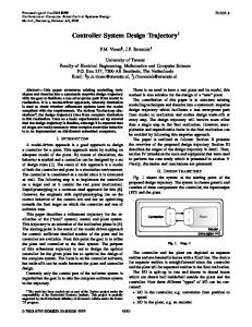
Preliminaries Before addressing the above problem, it is instructive to examine briefly the various mechanisms of heating. Figure 1 shows, on an exaggerated scale, a cutaway section of the vehicle and the shock layer around it. The primary mechanism of heating at the surface is a combination of convection and mass diffusion, due to temperature and species concentration gradients, respectively, in the wall-bounded shear layer. Another mechanism is interaction between the wall material and the hot gas adjacent to it – some wall materials promote the recombination of atomic species, and the consequent energy release adds to the heating at the wall. This phenomenon, called surface catalysis, is an important consideration in aerothermal design. Yet another mechanism is radiation from the shock layer in the case of flows with sufficiently large energy. The primary requirement of the computational tools is that they accurately predict these various heating mechanisms. Note that the term “accuracy” is a rather broad one, and includes both numerical accuracy, and that of the mathematical model representing the flow and its interaction with the TPS material. One should recognize that aeroheating of the flight vehicle is strictly a time-dependent process. Initially, the material making up the thermal protection system is at low temperature and “soaks up” the entry heat – the conductivity of the material transports the heat (from the vehicle surface) through the thickness. The material will also re-radiate some of the heat back to the flow – the amount depending on the emissivity of the material. It is also possible that the TPS material could degrade through ablation (i.e., melting, vaporization, pyrolysis, etc.). No matter what the heating mechanism or material response, it is of utmost importance to keep the bond line (see Figure 1) at, or below, a reasonable temperature. The bond line represents the interface between the external (TPS) and internal (structures, etc.) thermal environments. Almost all TPS sizing computations are performed subject to the constraint that the bond line temperature not exceeding a specified value. It must be noted that the preceding discussion assumes that the TPS is not a load bearing subsystem of the vehicle. Another point to consider from the preceding discussion – the flow, its interaction with the material, and the response of the material, are coupled processes that require a time-dependent approach. Such an approach can get prohibitively expensive, especially at the preliminary
7-2
RTO-EN-AVT-116
System Design Constraints – Trajectory Aerothermal Environments
design stage in which the choice of TPS material(s) is not specified, and the predicted aerothermal environments are necessary to guide the selection. Therefore, flow computations and material thermal response computations are performed in an uncoupled manner, i.e., aerothermal/CFD computations are performed along a trajectory assuming a non-conducting TPS material, which is an adiabatic back wall assumption. Material response computations are performed a posteriori from the surface aerothermal environments obtained from the CFD computations. In this uncoupled approach, aerothermal analyses (under a steady flow assumption at a given time) are performed at several time points on the flight trajectory. The “discrete” time history of surface heating is then used in the in-depth conduction problem for specified materials (known properties). It is very tempting to select a large number of points (with fine granularity in the time parameter) to perform aerothermal calculations. However, a large number of simulations will prove neither cost effective nor timely in the preliminary design stage in which quick turnaround of heating estimates is necessary. The approach one could (perhaps should) take is to employ approximate/engineering methods to a larger degree than CFD. Maximum benefits accrue from the engineering methods that are “anchored” or calibrated to the more accurate CFD results. The emphasis in the present paper is on the use of a combination of CFD and engineering methodology to help in the definition of aerothermal environments suitable for designing the TPS of a hypersonic flight vehicle. The X-33 vehicle is used an example to demonstrate this approach [3, 4]. While the paper assumes (Earth) atmospheric flight, the methodology can be applied to entry/flight in any planetary atmosphere as long as an adequate model is available for it. The present paper is neither a comprehensive document on various approaches to the design problem, nor one drawn exclusively from personal experience. The paper does represent, however, the collective experience of one small team at NASA Ames Research Center. A more comprehensive review of CFD computations for hypersonic vehicles can be found in the paper of Gnoffo et al. [5].
Requirements The broad statement of the aeroheating problem assumes as given, a configuration and a flight trajectory. The following discussion should help sharpen the focus at little more by placing additional requirements on the configuration and trajectory. Configuration The uncoupling of the thermal response computations from the flow computations implies that it is sufficient to predict the heating at the outer surface (Outer Mold Line or OML) of the configuration. The configuration is provided usually in some CAD (Computer-Aided Design) format and the OML has to be extracted from it – the CAD model will contain more details than are necessary for aerothermal analysis. One of the biggest difficulties generally is that different CAD packages have different file formats, and translating these formats can be time
RTO-EN-AVT-116
7-3
System Design Constraints – Trajectory Aerothermal Environments
consuming. Assuming that the CAD model is available in a suitable format, a “water tight” OML is obtained by “stitching” together the defining surfaces, and closing gaps as necessary, or as dictated by specific requirements. Further, geometric simplifications or additional surfaces may be necessary from the point of view of grid generation. It is assumed that such modifications will have little or no impact on the aerothermal environment. The water tight OML forms the basis for generating volume meshes [6] for aerothermal simulations. Trajectory Aerothermal CFD simulations require – (1) flight speed (or Mach number), (2) freestream density, (3) freestream temperature, (4) freestream gas composition, and (5) vehicle attitude (angle of attack and/or yaw angle). The flight trajectory commonly contains the time history (usually from atmospheric entry interface to landing) of position (altitude and geographical coordinates), velocity (inertial or relative), and attitude of the vehicle. Knowing the altitude, one can obtain the time histories of mass density and temperature using an appropriate (or standard) atmospheric model. Thus, a complete set of CFD input data are available at every point along the trajectory. In addition to these data, one can make preliminary estimates of the convective heat flux at the stagnation point of a sphere of specified radius (Rn is usually 1 m or 1 ft) using some variant of the Fay-Riddell correlation [7], which is based on boundarylayer analysis for chemically reacting air. Briefly, the stagnation point convective heat flux (to a cold wall) is inversely proportional to the square root of the radius, and directly proportional to the freestream density and velocity raised to some power m and n, respectively, i.e., C m n q&0,conv = conv (ρ∞ ) (V∞ ) (1) Rn where, m = 0.5, n ≈ 3-3.15, and Cconv is the constant of proportionality. For the case of radiation equilibrium, an implicit implementation of the above yields the stagnation point “hot wall” convective heat flux. The implicit implementation (in T0) is C h (T ) ⎤ m n⎡ q&0,conv = ε σ T04 = conv (ρ∞ ) (V∞ ) ⎢1 − w 0 ⎥ (2) H∞ ⎦ Rn ⎣
where, ε (0 ≤ ε ≤ 1) is the emissivity of the surface. A typical value of emissivity is 0.85. Note, for surfaces that are not efficient at re-radiating heat (i.e., low emissivity) the stagnation point flux is higher than that for a surface of emissivity closer to 1 – one would like to choose a material/surface coating of very high emissivity to decrease heating. The review paper of Tauber [8] has more details of various methods to estimate the stagnation point convective heat fluxes for air (and other gas mixtures). The stagnation point radiative heat flux, unlike the convective, is directly proportional to the nose radius. Following Martin [9] m n q&0, rad = Crad Rn (ρ∞ ) (V∞ ) (3) where, m = 1.6, n ≈ 8.5, and Crad is the constant of proportionality. A more recent paper of Tauber and Sutton [10] provides useful correlations for stagnation point radiative heat flux for Earth and Mars entries. Radiative heating is a complex topic that deserves a paper of its own. For the present, it is assumed that heating due to shock-layer radiation can be neglected.
7-4
RTO-EN-AVT-116
System Design Constraints – Trajectory Aerothermal Environments
Knowing the freestream density, flight speed, nose radius, and enthalpy variation with temperature, the stagnation point radiative equilibrium temperature (or equivalently, the convective heat flux) can be computed. Figure 2 schematically illustrates the stagnation-point heat flux history for a typical non-lifting entry. Note the build up of heat flux with increasing time of flight. The heat flux reaches a peak value at some point (time) on the trajectory, and decreases continually past that. It is now obvious that the set of trajectory points selected for aerothermal analysis should include the peak heating point at a minimum. However, the peak heat flux is only one criterion in the design of the TPS – choice of material to withstand the predicted heat flux. The other important criterion is the area under the heat flux curve (shown shaded in Fig. 1 and as a curve of growth – dashed line). This area is also termed integrated heat load, i.e. tf
r r Q(r ) = ∫ q& (r ; t )dt
(4)
ti
While the peak heat flux guides the selection of TPS material type, the integrated heat load determines the thickness of the TPS material. Therefore, the points selected on the trajectory for CFD analysis should be chosen to replicate the area under the heat pulse. The leftmost point (early on the trajectory) on the heat pulse is chosen from continuum considerations, i.e., the point is chosen so that Knudsen number based on the vehicle characteristic dimension does not exceed 0.001 and the convective heat flux has a “reasonable value.” The rightmost point on the heat pulse is chosen from either a desired dynamic pressure, or Mach number limit (e.g., M∞ ≤ 4), and the other points are distributed between these three. A more detailed discussion of trajectory point selection is deferred until later.
CFD Modeling & Numerics The flight through the atmosphere of the hypersonic vehicle experiences different flow regimes ranging from free molecular flow at very high altitudes to complete continuum deep in the atmosphere. The physical models are different in these different flight regimes, and pose a challenge to developing a single numerical methodology to encompass them all. Fortunately, most of the heating occurs in the continuum regime, and CFD codes that solve the Navier-Stokes equations (with appropriate physical models for shock-layer processes) are adequate. Each constituent species if the gas mixture is assumed to be thermally perfect, and the main requirements for the models in the continuum simulations are – (1) thermodynamic and transport (mass, momentum, and energy) properties of the constituent species, (2) accurate representation of reactions, and their associated rates, in the shock layer, and (3) models for thermal nonequilibrium, if necessary. The last one is necessary if preliminary computations (Eq. 3) indicate substantial radiative heating. Simple one-dimensional equilibrium computations for a normal shock corresponding to the freestream conditions at the trajectory points yield useful information about the post-shock distributions of species and thermodynamic states. The data obtained provide rough guidelines as to which model is appropriate for the computations, e.g., should one consider air to be a mixture of 5, 7, or 11 species. The important aspects of physical modeling will not be elaborated upon here because RTO-EN-AVT-116
7-5
System Design Constraints – Trajectory Aerothermal Environments
they are addressed either in earlier papers [11, 12], and in several texts [13–16]. There are, however, three important modeling issues that need further attention – (1) gas-surface interaction, (2) transition, and (3) turbulence. r Consider the surface boundaryr conditions. Apart from the usual “no-slip” ( uw = 0 ), and r zero normal pressure gradient ( ∇p ⋅ nw = 0 ) boundary conditions at the surface, mass and energy balance equations are necessary to represent the interaction of the gas and surface. Firstly, the mass balance equations are obtained from the statement that the flux due to mass diffusion is balanced by the production of molecular species through recombination of atoms r r RTw (5) J s w ⋅ nw = ρ s w γ s (Tw ) 2π M s If γs = 1, the surface is said to be fully catalytic, i.e., the surface permits complete recombination of atoms arriving at the surface, and if γs = 0, the surface is said to be noncatalytic, i.e., the surface does not permit recombination. The heat released due to recombination is a maximum for a catalytic surface, and zero for a noncatalytic one. For a real material, the recombination coefficients lie in between the two extremes, i.e., 0 ≤ γs ≤ 1 and are characteristic of that material. Further, these coefficients are functions of temperature, i.e., γ s = γ s (T ) . For the purposes of initial TPS design studies, the conservative assumption of a fully catalytic surface is preferred since one can expect maximal heat release from recombination. Note that in the case of air, the surface is assumed to be noncatalytic to NO and permits only recombination of N and O. Secondly, radiative equilibrium is assumed to exist at the wall, i.e., the total heating to the wall composed of conductive and catalytic heating is assumed to be equal to that re-radiated from the surface. The energy balance equation at the surface is, therefore, r r r r n − κ w∇T ⋅ nw + ∑ s =s 1 hs (Tw ) J s w ⋅ nw = ε w (Tw ) σ Tw4 (6) 14243 144 42444 3 14243 convective
diffusion
re − radiation
where, the emissivity, in general, is a function of temperature and again, this functional variation depends on the type of material. Note that Eq. 6 ignores in-depth conduction through the TPS. The other important issues that affect the convective heating at the wall are transition and turbulence. Since the onset of transition cannot be predicted a priori, the results from laminar computations are post-processed for boundary-layer momentum thickness and edge Mach number. The ratio of the momentum thickness Reynolds number to the edge Mach number is used as a guide to determine the onset of transition empirically through correlation of computed laminar boundary-layer parameters (notably the momentum thickness) with experimental data (e.g., see Ref. 17). Note that this is only one of many criteria, and assumes the body is smooth. Irregularities in the surface – either roughness or steps/gaps – could cause transition to occur earlier. Assuming that onset of transition can be determined using the momentum thickness Reynolds number criterion, the length of the transition region must be predicted. The issue of transition is beyond the scope of the present paper, and will be covered
7-6
RTO-EN-AVT-116
System Design Constraints – Trajectory Aerothermal Environments
in a companion lecture [18]. For the lack of a good transition model, the assumption of a fully turbulent flow is usually made, and an algebraic turbulence model is used, e.g., the BaldwinLomax model [19] corrected for compressibility [20] – reasonably good for attached flows but not so for separated leeside flows. Such an assumption can lead to excessive conservatism in the design of the TPS – simply due to predicted high levels of heating in forward part of the configuration. Undoubtedly, there are more sophisticated turbulence models available. Whether or not they are cost effective in the preliminary design stage is debatable given the advances in computer hardware. It is assumed that a computer program (commercial or otherwise) incorporating the necessary model is readily available to compute the various cases. Most of the recent flow solvers are solve the Navier-Stokes equations in a finite-volume formulation, and use some form of upwinding – essentially some approximate solver to a one-dimensional Riemann problem [21].
Grid Generation The most important single step in any computational analysis of the flow field is that of building a volume mesh. This can be a time-consuming process, especially if the configuration is complex. A grid topology has to be developed first. For the cases with no sideslip, it is sufficient to build a topology over either the port or starboard half of the vehicle. The distribution of surface grid points is dictated by the level of resolution required in various areas, e.g., the bow shock-wing shock interaction region for a winged vehicle requires fine resolution. Since the volume mesh generation takes a long time for a complex configuration (or grid topology), the strategy usually adopted is to build one volume mesh, which can be tailored for various flow conditions. The requirements are that the mesh be large enough to accommodate the lowest Mach number, and the highest and lowest angles of attack. The distribution of grid points in the wall-normal direction are driven by the freestream Reynolds number – high Reynolds numbers requiring adequate spacing to resolve the thin shear layer bound to the wall. Initial computations are performed on this single grid (also referred to as the master grid) for all points on the trajectory. The grid is then tailored for the freestream conditions at each selected trajectory point. This second round of computations can be avoided if the CFD software has the ability to tailor the grid as part of the flow solution process itself. A detailed exposition of requirements and strategies for grid generation for hypersonic flows is in the paper of Papadopoulos et al. [6].
Engineering Methodology The aerothermal computations provide various surface quantities such as temperature, heat flux, shear stress (or force), etc., as functions of the trajectory time parameter, t. However, there are only a finite number of time points, and one requires the aerothermal environments over the entire trajectory. In the early design stages, which require very rapid turnaround of
RTO-EN-AVT-116
7-7
System Design Constraints – Trajectory Aerothermal Environments
environments for trade studies, it is most cost effective to supplement accurate CFD-based analyses with engineering methodology. Engineering methods allow for finer granularity in the trajectory time parameter. Since engineering methods are usually based on empirical correlations or other approximations, it is important that such methods be anchored or calibrated against the more accurate CFD results. The calibrated engineering tool serves as both an interpolation and extrapolation tool – interpolation being used between points at which CFD computations have been performed, and extrapolation in regions outside (typically low altitude supersonic and subsonic Mach numbers). Such an approach was adopted for the X-33 program, in which an engineering code was used [22]. This approach is described here briefly. One must first recognize that the aerothermal environments (meaning surface quantities such as pressure, temperature/heat flux, shear stress/force, etc.) depend on the freestream Mach number, Reynolds number (or dynamic pressure), and angle of attack, i.e., if S represents a surface quantity, then the functional dependence of the quantity is mathematically expressed as r r S (r ; t ) = S (r ; M (t ), q (t ), α (t )) (7) Using engineering correlations and approximate theories (impact theories), the engineering code can rapidly develop a database of surface quantities from the three freestream parameters M, q , and α to a user-specified fineness in the time parameter t. Transition and turbulence are included empirically, and a specified time interval is used as the interval between onset to fully-developed turbulence. The laminar and turbulent CFD solutions are then used in the interpolation process. The fundamental idea behind the engineering method is one of scaling dynamic pressure being the scaling variable. Additional details of the engineering method are available in the paper of Kontinos et al. [23].
Case Study: X-33 The X-33 program was a NASA – Lockheed-Martin partnership to build a sub-orbital flight demonstrator (half-scale prototype of a Re-usable Launch Vehicle or RLV). Based on the concept of a lifting body, the X-33 flight vehicle (two candidate configurations are shown in Fig. 3) had several innovative technologies including composite structures and integrated cryotanks, linear aerospike engine, and metallic TPS. Although the X-33 program has been cancelled, the aerothermal analysis methodologies developed are still of value. For the X-33, aerothermal analyses were performed in two ways – (1) along design trajectories, and (2) in a design space – both of which are discussed here. Trajectory Based Approach to Aerothermal Design
In the trajectory-based approach, aerothermal computations are performed at a finite number of “critical” points on the given trajectory. An engineering method, anchored to the
7-8
RTO-EN-AVT-116
System Design Constraints – Trajectory Aerothermal Environments
computed solutions, is used to reconstruct the aerothermal environments along the entire trajectory. Figure 4 shows the various parameters of the X-33 design trajectory. Shown as open symbols in Figure 4, are the points that were selected for CFD computations. Figure 4a shows the history of cold wall convective heat flux at the stagnation point of a reference sphere (Rn = 0.3048 m). Figures 4b through 4e show the time histories of altitude, Mach number, angle of attack, and unit Reynolds number. The points selected for CFD adequately represent the heat pulse. In addition to the peaks on the heat pulse, the other points selected included the peak Mach number, highest angle of attack, highest dynamic pressure (for a freestream Mach number above 6), and a point at which the Mach number is high and the angle of attack is low. This last point was considered critical from the point of view of shock-shock interaction heating at the leading edge of the canted fin – the worst heating occurs at the lowest angle of attack since the shock impingement is closer to the geometrical leading edge where the radius is the smallest (hence highest heating). The dashed line in Fig. 4e specifies the unit Reynolds number above which the flow is assumed fully turbulent. A CFD point selected that lies above this line require a turbulent flow computation in addition to a laminar one. The trajectorybased approach followed for the X-33 is schematically shown in Fig. 5. The computed CFD solutions were used to guide the selection of TPS materials and splitlines (boundaries separating dissimilar TPS materials). One way of selecting the splitlines is to extract, at each point on the surface, the maximum temperature (or heat flux) over all time. The surface contours of the maximum temperature indicate how the heating varies on the surface (see Ref. 3). This was the initial procedure followed for the X-33. However, detailed examination of the surface heating over the trajectory led to the choice of splitlines being made from the results at the peak turbulent heating point. The temperature contour lines corresponding to 500, 750, 1500, 1650, and 1900 °F (533, 672, 1089, 1172, and 1311 K) are shown in Figure 6. These values were assumed multi-use temperature limits of candidate TPS materials. Note that the CFD computations did not account for any in-depth conduction through the material. The actual splitlines were based on the true radiative equilibrium temperatures obtained through application of thermal analysis tools that accounted for heat soak through the thickness. Verification computations should be performed with the material map. Such computations would have to consider the finite catalycity (γs(T) < 1) and emissivity of the actual TPS materials. A limited set of computations were performed for the splitlines at the nose region for the X-33 [24]. At the peak laminar heating point (M∞=11.4, α=35.8º) on the X-33 design trajectory, CFD computations were performed assuming two different materials maps. One material map assumed the nose cap and aeroshell were both fully catalytic, and the other assumed the nose cap material to be RCG (Reaction Cured Glass) which was used on the Space Shuttle and the aeroshell TPS material to be coated with a more catalytic material (Pyromark 2500). The surface isotherms for the two different surface materials maps are
RTO-EN-AVT-116
7-9
System Design Constraints – Trajectory Aerothermal Environments
compared in Fig. 7. A few interesting features must be noted. Firstly, the assumption of RCG kinetics for the nose cap reduces temperatures significantly because the material does not promote atomic recombination as much as a fully catalytic material does. However, when the free atoms traverse the interface between the noncatalytic and catalytic material, they undergo recombination. Consequently, there is a sudden increase in temperature across the interface. This increase is called a catalytic “jump” requires fine grid spacing across the interface for good resolution. Since the CFD computations do not include in-depth conduction, nothing can be said about the magnitude and accuracy of the temperature rise. Note that the magnitude of the temperature jump can exceed the fully catalytic value – calling into question the conservatism in the assumption of a fully catalytic wall. One of big sources of uncertainties in the aerothermal simulations is lack of precise knowledge of surface materials and their interaction with the shock layer gas. Other than the definitive flight experiment of Stewart et al. [25], there have not been focused flight experiments to measure or quantify catalytic heating. The computed CFD solutions can also guide the layout of TPS panels. The layout of the panels is dictated by the local flow direction. The ideal choice is to have the flow go diagonally across a panel. Figures 8a and 8b show perspective views of the streamline patterns at the peak laminar and turbulent (M∞=10, α=20º) heating points, respectively, on the design trajectory. The surface streamline patterns strongly depend on the angle of attack, and it is not possible to meet the flow direction constraint in designing an optimal layout of panels. Design Space Based Approach to Aerothermal Design
The preceding discussion assumed that a trajectory was available for the given flight configuration. The tacit assumption is that the aerothermal environments on the trajectory do not exceed, either single-use or multi-use, temperature limits of the TPS material. In reality, flight trajectories must be constrained by the aerothermal performance of the TPS material. This circular argument clearly points out the need for an alternate method – one in which computed aerothermal environments could be used to constrain and develop optimal flight trajectories. Just such an alternate approach – the Design Space approach – was developed during the X-33 program [3]. The essence of this approach is decoupling trajectory development from the definition of aerothermal environments, i.e., aerothermal databases are computed a priori to provide constraints to trajectory development. The most important parameters that affect surface heating are the freestream Mach number, unit Reynolds number, and angle of attack (and perhaps, sideslip angle). A Design Space represented by these three parameters is constructed to accommodate or enclose all possible flight trajectories. The Design Space has to be large enough to accommodate trajectory dispersions – at least at high Reynolds numbers. CFD simulations are performed at several discrete points in this Design Space, and the results are used to anchor the engineering
7 - 10
RTO-EN-AVT-116
System Design Constraints – Trajectory Aerothermal Environments
method. The main advantage of the Design Space approach is that the engineering method, calibrated using the CFD results, can now provide aerothermal environments for any flight trajectory in a timely manner. The main disadvantage is that the Design Space is tightly linked to a configuration, i.e., if the configuration undergoes any major changes, then the Design Space will have to be refined and CFD computations performed again. Note that the Design Space is multi-dimensional, and the point distribution needs to be regularly spaced or clustered in regions where rapid changes are expected. Strictly speaking, it is better to work in a truly orthogonal space, i.e., with flight speed, freestream density, and angle of attack (and sideslip) as the independent coordinates. For one X-33 configuration, the Design Space is graphically depicted in Figs. 9a through 9c. The Design Space covers a Mach number range from 2 to 15, an angle of attack range from 0º to 45º, and a Reynolds number range of 13,000/m to 3,200,000/m. The points selected in this Design Space are indicated as closed symbols in the figures. Note that the solutions computed along the design trajectory can also be included in the Design Space, thus increasing the point density. The selection of Mach numbers is straightforward. Increased point density in angle of attack is necessary to capture fluid dynamic phenomena – streamlines, separation and attachment lines being strongly dependent on angle of attack. The solutions computed in the Design Space help establish the various trends and bring into focus the linear or nonlinear dependence of aerothermal environments to critical design parameters. The Design Space approach used in the X-33 program is schematically summarized in Fig. 10. As mentioned earlier, the Design Space approach uncouples aerothermal analyses from trajectory development. The problem of computing aerothermal environments for a given trajectory can now be inverted, i.e., given the aerothermal environments one can develop trajectories subject to the constraints that no violations of TPS temperature limits are permissible. In principle, one would like the trajectory development to include the aerothermal environment at every surface mesh point on the vehicle surface as a constraint. Such an approach would get unwieldy very quickly. Instead of using all points on the body surface, a few key points are used. The environments at these key points, often referred to as body points, can be integrated as constraints into the trajectory programs. In other words, the trajectory programs now have both an aerodynamics and an aerothermodynamics database to work with. For the X-33 configuration, 10 thermal control body points (Fig. 11) were used. These points were selected at on the windward and leeward centerlines and at the leading edge of the canted fin.
Summary A large part of the discussion is summarized in Fig. 12, which schematically lays out the process for generating aerothermal environments along trajectories using a combination of CFD and engineering methods. For a given configuration (or equivalently a volume mesh),
RTO-EN-AVT-116
7 - 11
System Design Constraints – Trajectory Aerothermal Environments
the freestream conditions, and, perhaps, a specification of surface materials are used by the CFD solver to generate aerothermal environments (surface temperatures, heat fluxes, streamlines, surface pressure and shear loads – hence aerodynamic force and moment coefficients) at several points on a given flight trajectory. Accurate environments can be obtained if the four major components of the solver – the thermodynamics, transport, shocklayer chemical kinetics, and surface catalysis models are representative of the flow. The environments obtained from CFD are used to anchor the engineering method, which is then used to generate aerothermal environment along the entire trajectory. The computed environments can then be used to determine the TPS splitlines and layout, or given a TPS layout, environments can be computed for actual surface materials. A Design Space approach that uncouples the process for defining the aerothermal environments from trajectory development is introduced. The advantage of building an environments database from the Design Space is that aerothermal performance constraints can be used in developing trajectories that do not unduly stress the TPS. The only disadvantage of the Design Space approach is that resulting database is tightly linked to a configuration and requires redefinition if the configuration changes.
Acknowledgements The author was supported by NASA Ames Research Center, through a contract NAS2-99092 to ELORET Corp. The author would like to thank his colleagues in the Reacting Flow Environments Branch at NASA ARC for the fruitful partnerships, and their suggestions and insights.
References 1. Fletcher, D. G., “Fundamentals of Hypersonic Flight – Aerothermodynamics,” Critical Technologies for Hypersonic Vehicle Development Technology – RTO/AVT/VKI Lecture Series, 10-14 May 2004, Von Karman Institute for Fluid Dynamics, Brussels, Belgium. 2. Dorrance, W. D., Viscous Hypersonic Flow. McGraw-Hill, New York, 1962. 3. Prabhu, D. K., Loomis, M. P., Venkatapathy, E., Polsky, S., Papadopoulos, P., Davies, C. B., and Henline, W. D., “X-33 Aerothermal Environment Simulations and Aerothermodynamic Design,” AIAA Paper No. 98-868, January 1998. 4. Bowles, J. V., Henline, W. D., Huynh, L. C., Davies, C. B., Roberts, C. D., and Yang, L. H., “Development of an Aerothermodynamic Environments Database for the Integrated Design of a Prototype Flight Tests Vehicle,” AIAA Paper No. 98-0870, January 1998. 5. Gnoffo, P. A., Weilmuenster, K. J., Hamilton, H. H., II, Olynick, D. R., and Venkatapathy, E., “Computational Aerothermodynamic Design Issues for Hypersonic Vehicles,” J. Spacecraft and Rockets, Vol. 36, No. 1, 1999, pp. 21-43.
7 - 12
RTO-EN-AVT-116
System Design Constraints – Trajectory Aerothermal Environments
6. Papadopoulos, P., Venkatapathy, E., Prabhu, D., Loomis, M. P., and Olynick, D., “Current Grid-Generation Strategies and Future Requirements in Hypersonic Vehicle Design, Analysis and Testing,” Appl. Math. Modeling, Vol. 23, 1999, pp. 705-735. 7. Fay, J. A., and Riddell, F. R., “Theory of Stagnation Point Heat Transfer,” J. Aero. Sci., Vol. 25, No. 2, 1958, pp. 73-85. 8. Tauber, M., “A Review of High-Speed, Convective, Heat-Transfer Computation Methods,” NASA TP 2914, 1989. 9. Martin, J. J., Atmospheric Re-entry, an Introduction to Its Science and Engineering. Prentice-Hall, Inc., Englewood Cliffs, New Jersey, 1966. 10. Tauber, M., and Sutton, K., “Stagnation Point Radiative Heating Relations for Earth and Mars Entries,” J. Spacecraft and Rockets, Vol. 28, No. 1, pp. 40-42, 1991. 11. Magin, T., and Barbante, P. F.., “Fundamentals of Hypersonic Flight – Properties of High Temperature Gases,” Critical Technologies for Hypersonic Vehicle Development Technology – RTO/AVT/VKI Lecture Series, 10-14 May 2004, VKI, Brussels, Belgium. 12. Longo, J., “Modeling of Hypersonic Flow Phenomena,” Critical Technologies for Hypersonic Vehicle Development Technology – RTO/AVT/VKI Lecture Series, 10-14 May 2004, VKI, Brussels, Belgium. 13. Anderson, J. D., Jr., Hypersonic and High Temperature Gas Dynamics, McGraw-Hill, New York, 1989. 14. Park, C., Nonequilibrium Hypersonic Aerothermodynamics, John Wiley & Sons, New York, 1990. 15. Bertin, J. J., Hypersonic Aerothermodynamics, AIAA Education Series, AIAA, Washington, DC, 1994. 16. Bose, T. K., High Temperature Gas Dynamics: An Introduction for Physicists and Engineers, Springer Verlag, Berlin, 2004. 17. Horvath, T. J., Berry, S. A., Hollis, B. R., Liechty, D. S., Hamilton, H. H., II, and Merski, N. R., “X-33 Experimental Aeroheating at Mach 6 Using Phosphor Thermography,” AIAA Paper 99-3558, June 1999. 18. Arnal, D., and Delery, J, “Fundamentals of Hypersonic Flight – Fluid Dynamics – SWBLI and Transition,” Critical Technologies for Hypersonic Vehicle Development Technology – RTO/AVT/VKI Lecture Series, 10-14 May 2004, VKI, Brussels, Belgium. 19. Baldwin, B. S., and Lomax, H., “Thin Layer Approximation and Algebraic Model for Separated Turbulent Flows,” AIAA Paper No. 78-257, January 1978. 20. Prabhu, D. K., Wright, M. J., Marvin, J. G., Brown, J. L., and Venkatapathy, E., “X-33 Aerothermal Design Environment Predictions: Verification and Validation,” AIAA Paper 2000-2686, June 2000. 21. Toro, E., Riemann Solvers and Numerical Methods for Fluid Dynamics, SpringerVerlag, Berlin, 1997. 22. Bowles, J. V., Henline, W. D., Huyhn, L. C., Davies, C. B., Roberts, C. D., and Yang, L. H., “Development of an Aerothermodynamic Environments Database for the
RTO-EN-AVT-116
7 - 13
System Design Constraints – Trajectory Aerothermal Environments
Integrated Design of the X-33 Prototype Flight Test Vehicle,” AIAA Paper No. 98-870, January 1998. 23. Kontinos, D. A., Wright, M. J., Prabhu, D. K., and Venkatapathy, E., “X-33 Aerothermal Design Environment Predictions: Review of Acreage and Local Computations,” AIAA Paper 2000-2687, June 2000. 24. Prabhu, D. K., Venkatapathy, E., Kontinos, D. A., and Papadopoulos, P., “X-33 Catalytic Heating,” AIAA Paper 98-2844, June 1998. 25. Stewart, D. A., Rakich, J. V., and Lanfranco, M. J., “Catalytic Surface Effect Experiment on Space Shuttle,” in Progress in Aeronautics and Astronautics (T. E. Horton, ed.), Vol. 82, pp. 248-272, AIAA, New York, 1982.
7 - 14
RTO-EN-AVT-116
System Design Constraints – Trajectory Aerothermal Environments
Shock wave
Shock layer
TPS
Radiation In-depth conduction Convection Diffusion Recombination
V
Bond line
α
Re-radiation
3
2x10
1200
Figure 1. Schematic diagram illustrating various heating mechanisms. The bond line refers to the interface between the thermal protection system and the interior of the flight vehicle.
Heat load
0
0
2
200
8Convective 6 heat load4
Convective heat flux 400 600 800
10
1000
Heat flux
0
5
10
15
20
25 Time
30
35
40
45
50
Figure 2. Schematic diagram illustrating the time history of convective heat flux at the stagnation point of sphere for nonlifting entry. The dashed line represents the time integral of the heat flux, i.e., heat load. The value of the heat load is the value of the area (shown shaded) under the heat flux curve.
RTO-EN-AVT-116
7 - 15
System Design Constraints – Trajectory Aerothermal Environments Vertical tail
Canted fin
Aeroshell
Figure 3. Two X-33 configurations for acreage aerothermal computations. The configurations do not include the body flaps at the aft end. The gaps between the control surfaces on the wing are also closed (Ref. 3). 50 Trajectory Selection for CFD
2
Reference heating rate, q (W/cm )
40
30
20
10
Area under the curve is the integrated heat load
0 0
200
400
600
800
Time, t (s)
(a) Reference heat flux history – stagnation point of a sphere of radius 0.3048 m (1 ft) 100
16 Trajectory Selection for CFD
Trajectory Selection for CFD 14
80
Mach number, M∞
Altitude, Z (km)
12
60
40
10
8
6
4 20 2
0
0 0
200
400
600
800
0
200
Time, t (s)
400
600
800
Time, t (s)
(b) Altitude history
(c) Mach number history 8
50
10 Trajectory Selection for CFD
Trajectory Selection for CFD
40
7
Unit Reynolds number, Re∞ (1/m)
Angle of attack, α (deg)
10
30
20
10
6
10
TURBULENT
5
10
LAMINAR
4
10
0
3
-10
10 0
200
400
600
Time, t (s)
(d) Angle of attack history
800
0
200
400
600
800
Time, t (s)
(e) Unit Reynolds number history
Figure 4. The X-33 reference trajectory used in design aerothermal computations. The solid line corresponds to the flight trajectory, and the open symbols represent trajectory points selected for acreage aerothermal computations (Ref. 3).
7 - 16
RTO-EN-AVT-116
System Design Constraints – Trajectory Aerothermal Environments
INPUTS Trajectory
INPUTS "SMOOTH" OUTER MOLD LINE
Conditions at Selected Trajectory Point (ρ∞, T∞, V∞, α)
CFD ANALYSIS Entire Vehicle Aerothermal Environment at Trajectory Points
ENG. TOOL Heating Environments Along Entire Trajectory
Vehicle Thermal Model Structural Loads
Figure 5. Schematic diagram of the trajectory-based approach. CFD computations are performed at several points on a given trajectory. Using the CFD solutions as anchor points, the engineering method then generates aerothermal environments for the entire trajectory (Ref. 3).
WINDSIDE VIEW
LEESIDE VIEW SIDE VIEW
Figure 6. Isotherms (radiative equilibrium with emissivity = 0.85) of 500, 750, 1500, 1650, and 1900 ºF from CFD computations at the peak turbulent heating point of the X-33 design trajectory (Ref. 3).
RTO-EN-AVT-116
7 - 17
System Design Constraints – Trajectory Aerothermal Environments
RCG NOSE PYROMARK AEROSHELL
CATALYTIC NOSE CATALYTIC AEROSHELL Tw (°F) 2300
1800
1300
800
300
Figure 7. Contours of radiative equilibrium surface temperatures for two different surface materials maps – (1) ideal case of noncatalytic nose and catalytic aeroshell, and (2) RCG-coated nose and Pyromark 2500-coated aeroshell. The solutions correspond to the peak laminar heating point () on the X-33 design trajectory (Ref. 23).
(a) Surface streamline patterns for the X-33 configuration at the peak laminar heating point (M∞=11.4, α=35.8º)
(b) Surface streamline patterns for the X-33 configuration at the peak laminar heating point (M∞=10, α=20º)
Figure 8. Surface streamline patterns from CFD computations for the X-33 configuration at two trajectory points (Ref. 3).
7 - 18
RTO-EN-AVT-116
System Design Constraints – Trajectory Aerothermal Environments
100
60 Design Traj. Flt. Trajs. Design Space Pt.
Design Traj. Flt. Trajs. Design Space Pt.
50 80
Angle of attack, α (deg)
Altitude, Z (km)
40 60
40
30
20
10 20 0
0
-10 0
2
4
6
8
10
12
14
16
0
2
Mach number, M∞
(a) Altitude vs. Mach Number
4
6 8 10 Mach number, M∞
12
14
16
(b) Angle of attack vs. Mach number 8
10
Design Traj. Flt. Trajs. Design Space Pt. 7
Unit Reynolds number, Re∞ (1/m)
10
6
10
TURBULENT
5
10
LAMINAR
4
10
3
10
0
2
4
6
8
10
12
14
16
Mach number, M∞
(c) Reynolds number vs. Mach number
Figure 9. Design Space definition for the X-33 flight vehicle. Shown are – (a) the envelope of the altitude-Mach number space enclosing the design and candidate flight trajectories, (b) angle of attack-Mach number space, and (c) unit Reynolds numberMach number space (Ref. 3).
INPUTS "Smooth" Outer Mold Line
INPUTS
CFD ANALYSIS
Design Space (ρ∞, T∞, V∞, α)
Entire Vehicle Aerothermal Environment at Design Space Points
ENG. TOOL Heating Environments Along Entire Trajectory
Vehicle Thermal Model Structural Loads Trajectory Constraints
INPUTS Trajectory
OUTPUTS Aerothermal DB Entire Vehicle All Trajectories (including dispersions)
Figure 10. Schematic flow diagram of the Design Space approach. CFD analyses and trajectory definitions are decoupled. The engineering method, anchored to the CFD solutions, generates aerothermal environments for specific trajectories (Ref. 3).
RTO-EN-AVT-116
7 - 19
System Design Constraints – Trajectory Aerothermal Environments Nosecap 1
2
4 Aeroshell
Canted fin 3
6
5 7
WINDSIDE VIEW
LEESIDE VIEW Vertical tail
8 9 7
10
6 3 SIDE VIEW
Figure 11. Three views of the X-33 vehicle with locations of 10 thermal control body points. The darker areas represent the carbon-carbon TPS (ε=0.8) and the rest of the vehicle represents the metallic TPS or blankets (ε=0.6).
MODELING REFINEMENTS/VERIFICATION
CFD-BASED METHOD
AERODYNAMIC DESIGN CL, CD, CM
STRUCTURAL DESIGN Fp, Fµ
ENGINEERING METHOD
INPUTS
INPUTS
Configuration Materials Map Traj. Point or Design Space (ρ∞, T∞, V∞, α)
Configuration Materials Map Trajectory Point Transition Criteria CFD Solutions
CFD TOOL
ENG. TOOL
Thermodynamics Transport Chemical Kinetics Surface Catalysis
Correlations "Smart" Interpolation In-depth Conduction
OUTPUTS
OUTPUTS
Surface pressures Surface Temperatures Surface shear Aerodynamics Aerodynamic Loads Surface Oil Flow
Aerothermal DB Integrated Heat Loads
VEHICLE THERMAL DESIGN
TPS DESIGN Material Selection Splitlines Sizing Layout
Figure 12. Schematic diagram of inputs, major modeling assumptions, and outputs of CFD-based and engineering methods used toward the definition of aerothermal environments for a hypersonic flight vehicle.
7 - 20
RTO-EN-AVT-116