Convexity and optimization with copulÃ¦ structured ...

Technical report, 2016 A revised version of this manuscript will appear in Optimization

Convexity and optimization with copulæ structured probabilistic constraints W. van Ackooij1 & W. de Oliveira2 Abstract Probability constraints play a key role in optimization problems involving uncertainties. These constraints request that an inequality system depending on a random vector has to be satisfied with a high enough probability. In specific settings, copulæ can be used to model the probabilistic constraints with uncertainty on the left-hand side. In this paper we provide eventual convexity results for the feasible set of decisions under local generalized concavity properties of the constraint mappings and involved copulæ. The results cover all Archimedean copulæ. We consider probabilistic constraints wherein the decision and random vector are separated, i.e., left/right-hand side uncertainty. In order to solve the underlying optimization problem we propose and analyse convergence of a regularized supporting hyperplane method: a stabilized variant of generalized Benders decomposition. The algorithm is tested on a large set of instances involving several copulæ among which the Gaussian copula. A Numerical comparison with a (pure) supporting hyperplane algorithm and a general purpose solver for nonlinear optimization is also presented. Keywords Chance constrained programming – copulæ – joint chance constraints – second order conic programming – convexity – probabilistic constraints 1 EDF 2

R&D – 7 Boulevard Gaspard Monge 91120 Palaiseau, France UERJ - Universidade do Estado do Rio de Janeiro

1. Introduction In this work we are interested in optimization problems involving separable probabilistic constraints of the type P[ξ ≤ g(x)] ≥ p, Rn

Rm

(1) Rm

where g : → is a mapping having generalized concavity properties on a given level set, ξ ∈ is a random variable, P its associated probability measure and p ∈ (0, 1] a pre-specified probability level. Constraints of the form (1), also named chance-constraints or probabilistic constraints [43], express that the decision vector x ∈ Rn is feasible if and only if the random inequality system ξ ≤ g(x) is satisfied with high enough probability. These constraints are encountered in many engineering problems involving uncertain data. We can find applications in water management, telecommunications, electricity network expansion, mineral blending, chemical engineering etc. (e.g., [22, 38, 43, 59, 55]). For an overview of theory, numerics and applications of chance constraints we refer to [12, 43] and references therein. It is worthy mentioning that separable probabilistic constraints of the form (1) are not the most general class, but still a class widely present in relevant applications; see for instance [1, 55] for applications on power system optimization and [32] for chance constrained optimization applied to transportation problems. Although non trivial, chance constraints of the form (1) are easier to handle than more general chance constraints. We will assume throughout this paper that each component ξ i of the random vector ξ has a unidimensional continuous distribution function zi ∈ R 7→ Fi (zi ) := P[ξ i ≤ zi ], i = 1, ..., m. Therefore, Sklar’s Theorem [49] ensures that constraint (1) can be represented by a composite function involving the mapping g(x) = (g1 (x), . . . , gm (x)), the marginal distributions Fi , i = 1, ..., m, and a copula C : [0, 1]m → [0, 1]: P[ξ ≤ g(x)] = C(F1 (g1 (x)), ..., Fm (gm (x))) .

(2)

Under this notation, the optimization problem we are interested in is: min f (x) s.t. x ∈ X(p) ,

x∈Rn

(3a)

Convexity and optimization with copulæ structured probabilistic constraints — 2/24

where f : Rn → R is a convex function and, for a given p ∈ (0, 1], C(F1 (g1 (x)), ..., Fm (gm (x))) ≥ p , X(p) := x ∈ X gi (x) ≥ ì , i = 1, . . . , m

(3b)

with X a polyhedral set and ` ∈ Rm a given vector. An important matter for numerical tractability of chance-constrained optimization problems as (3) is convexity of its feasible set. In this work we will provide conditions under which X(p) given in (3b) is a convex set. These conditions involve generalized concavity of the composite function C(F1 (g1 (·)), ..., Fm (gm (·))), a threshold p∗ ∈ (0, 1] and a condition of the type p ≥ p∗ . Different copulæ C and different marginal distributions Fi provide different computable thresholds p∗ . The convexity results presented in this paper are essentially an extension of the work initiated in [24, 25, 56]. More specifically we show that all Archimedean copulæ belong to the class of δ -γ-concave copulæ introduced in [56]. In addition, we provide a stabilized variant of the supporting-hyperplane algorithm of [62], suitable for probabilistically constrained optimization problems with eventual convexity only. The new algorithm is combined with a generalized Benders decomposition that separates the potential non-convexity induced by the probability constraint from any inherent convexity of the nominal data. Prior to making this precise in Section 1.1 below, let us mention that [6] also considers copulæ in conjunction with probability constraints. This work, aiming to provide convexity results for probability constraints involving random technology matrices, seems to rely however on an unclear results on the independence of certain types of copulæ on the decision vector x ([6, Lemma 2.7]). This Lemma can be stated as follows: Consider the probability function Rn 3 x 7→ ϕ(x) = P[T x ≤ h], where the random K × n matrix T has rows following an elliptically symmetric distribution with positive definite covariance matrix. Then there exists a copula C independent of x such that ϕ(x) = C(Ψ1 (g1 (x)), ..., ΨK (gK (x))), where for each i = 1, ..., K, gi : Rn → R are deterministic mappings depending on hi and Ψi are x-independent marginal 1-dimensional distribution functions. This Lemma is false: Example 1. Assume that the 2 × 2 matrix T follows a multivariate Gaussian distribution centered in 0 with correlation matrix (when T is seen as a “vector” stored rows first):   1 0.75 −0.25 −0.10  0.75 1.0 −0.10 −0.25 , S= −0.25 −0.10 1.00 0.75  −0.10 −0.25 0.75 1.00 then T x is a centered 2-variate Gaussian random variable. Moreover P[T x ≤ h] = FΘ(x) ˜ (g1 (x), g2 (x)), ˜ ˜ 12 = where Θ(x) is a 2 × 2 correlation matrix having Θ(x)

−0.25x12 −0.25x22 −0.20x1 x2 , x12 +x22 +1.5x1 x2

hi , x12 +x22 +1.5x1 x2

gi (x) = √

i = 1, 2. (see, e.g.,

[54, proof of Theorem 3.2.4] for details on this derivation) and FΘ(x) is the 2-variate Gaussian distribution function of ˜ ˜ ˜ ˜ a centered Gaussian vector with correlation matrix Θ(x). Now the Gaussian copula CΘ(x) (defined as CΘ(x) (u1 , u2 ) := −1 −1 FΘ(x) ˜ (Φ (u1 ), Φ (u2 )), resulting from Sklar’s theorem, gives with u = (0.25, 0.25), x = (0, 1) and y = (0.75, 1): ˜

˜

CΘ(x) (u) = 0.0387 6= 0.0431 = CΘ(y) (u). Note that since 1-dimensional Gaussian distribution functions (denoted Φ above) are continuous, by [50, Corollary to Theorem 1], the Gaussian copula is the unique copula satisfying the requested representation. Hence this provides a concrete counterexample against the Lemma. The algorithms considered in [6] (the same are considered in [28]) are based on an ad-hoc implementation of a cutting plane method (with a priori generation of cutting planes) and a method seemingly related to p-efficient point approaches with interpolation (inner approximation). The convergence to an optimal solution is not established and the numerical experiments conducted on 5 instances indicate that the methods fail to close the gap below 2% on average. In contrast we provide a general optimization framework based on level bundle methods, establish convergence and show the interest of the methods on 1500 instances with respect to a competing standard software. We also mention the work [67] that uses a notion akin to g-concavity as introduced by [51] in order to generalize convexity results of probabilistically constrained feasible sets in the separable case (see also [56, Remark 3.3]). However they consider the situation of components-wise independence for the random vector ξ .


1.1 Separating out convexity Let us introduce extra variables u ∈ Rm to reformulate problem (3) as follows: vmin := min

u∈[0,1]m

v(u)

s.t.

C(u) ≥ p, and ui ≥ Fi (ì ), i = 1, . . . , m ,

(4a)

with objective function given by v(u) = min f (x) s.t. gi (x) ≥ Fi−1 (ui ), i = 1, . . . , m . x∈X

(4b)

The relation between formulations (3) and (4) is established in § 3.2. In the parlance of Bender’s decomposition, subproblem (4b) is denoted by slave problem and (4a) is the so-called master problem. Notice that the optimization of the slave problem is performed only in variable x, i.e., u is seen in (4b) as a parameter. Therefore, solving (4b) for a given u amounts to solving a convex optimization problem provided that f is a convex mapping and gi disposes of generalized concavity properties. As a result, any potential non-convexity of problem (3) has been moved to the master problem. This motivates us to solve (3) through an algorithm based on Bender’s decomposition. 1.2 Bender’s decomposition: a bird’s-eye view Generalized Bender’s decomposition – GBD – hinges on the key observation that certain problems can become significantly easier when a subset of variables is fixed. This observation originally made for problems with an underlying linear structure [3] potentially with stochastics [61] was generalized to problems with some underlying convexity in the seminal work by Geoffrion [20]. For a general overview we refer to [16, 8]. The optimal value of the slave problem is seen as a mapping of the fixed variables, called slave mapping or value function. The master problem is related to finding the optimal allocation of the previously temporarily fixed variables. It need not be a convex optimization problem. Since the domain of the value function need not be the whole space, the master problem is augmented with the so called feasibility cuts (i.e., an outer approximation of the convex domain of the value function). These can be computed using an auxiliary optimization problem involving slacks. The master problem is also enriched with optimality cuts, as a matter of fact, a cutting-plane model of the value function. In this view, GBD can be seen as a variant of the (Kelley’s) cutting-plane method given in [29]. It can therefore be subject to the well-known oscillation effect and slow convergence. In order to tackle this, the authors of [68] suggest what we would now call an inexact lower oracle (see [11]), i.e., inexactly solving the slave problem to compute some inexact but “cheap” cuts. An appropriate choice of cuts (approximating the value function) is crucial, as illustrated in [30]. The works [48, 47, 64, 13, 66] concretely deal with strategies for generating good (optimality) cuts, occasionally with a problem-dependent flavour. The authors of [7] are concerned with generating strong feasibility cuts and provide an important contribution in this view. Further improvements to the general scheme are concerned with a relaxation of the convexity assumption of the slave problem by allowing for integer variables [4] or the use of generalized “logic” duality (called inference duality) in [27]. The success of GBD is easily seen from the existence of many application, e.g., [46] or [53, 41, 21, 37, 15, 34, 5, 44, 39] just to name a few. To the best of our knowledge only a single work [69] deals with the study of GBD under generalized concavity properties. The authors suggest a layered Benders decomposition framework (two embedded Generalized Benders decompositions). In our setting, we cannot apply a cutting-plane method to solve the master problem because the Copula C in (4a) need not be concave. However, due to the generalized concavity assumptions on C, and provided that p ∈ (0, 1] is a large enough probability level (see Theorem 1 for more details), we rely on the supporting hyperplane method of [62] to solve problem (3) through Bender’s decomposition. 1.3 Main contributions and organization of the work In addition to theoretical results establishing δ -γ-concavity of all Archimedean copulæ (Theorem 2) and making explicit that it is sufficient for gi to dispose of generalized concavity properties on certain sets only (Theorem 1), we can enumerate the following contributions of this manuscript. 1.3.1 Contributions to supporting hyperplane and level bundle methods

In the present work, we rely on decomposition and employ a supporting hyperplane algorithms akin to [62] to find an optimal solution to problem (3) even when functions f and gi are nonsmooth. In contrast to [62] the proposed algorithm is able to handle extended real-valued objective functions. This is an important matter for dealing with value functions as in (4b). Another novelty with respect to [62] is that our algorithm employs a level-set regularization strategy similarly to [31] to avoid tailing-off effect that makes calculations unstable as the iteration process progresses. The algorithm is therefore an extension of level bundle methods [31, 57] to handle optimization problems having nonlinear constraints with generalized concavity properties and extended real-valued objective function. To the best of our knowledge, level bundle methods in the literature are only able to deal with: (a) linearly and nonlinearly constrained optimization problems involving convex functions, [31, 10]; or (b) linearly


constrained optimization problems with real-valued but quasi-convex objective function, [65]. In contrast to most level bundle methods in the literature that need to solve a QP master problem to define trial points, the proposed level bundle algorithm is general enough to define the master problem as a linear programming problem. This is an interesting feature when dealing with large-scale optimization problems. However, this feature might reduce convergence speed. 1.3.2 Contributions to the GBD literature

With respect to the existing literature on generalized Benders decomposition the contributions of the this work are as follows. We are concerned with local generalized concavity of mappings (generalized concavity of the mapping on certain level sets only). Compared to [69] we suggest a single layer framework. Moreover, we are interested in chance constrained problems with “left-hand side” uncertainty. To the best of our knowledge generalized Benders decomposition was not suggested for these problems before. With respect to this application, we incorporate in the master problem a special “feasible allocation” to avoid (possible) ill-conditioning related to stiff-gradients (see [35] and the discussion in [60]). The proposed algorithm combines in a single framework GBD, level bundle and supporting hyperplane methods. Although we have not investigated the enhancements related to appropriately selecting elements in the value function sub-differential, in the spirit of [33], we believe that this feature can be appended to the framework in a straightforward manner. 1.3.3 Organization

This paper is organized as follows: in Section 2 we present notation and several (already known) concepts. Section 3 is dedicated to convexity results: (a) of the set X(p) in (3b) provided p is large enough; (b) of the value function appearing in (4b). The algorithm and its convergence analysis are presented in Section 4. In Section 5 we approximate a very challenging chanceconstrained optimization problem by adopting the framework of problem (3) and consider such a reformulated/approximated problem in our numerical experiments. We also consider chance-constrained optimization problems arising from cascaded reservoir management (with real-life data). A comprehensive battery of experiments is presented in the same section, where we have also solved problem (3) by the nonlinear optimization solver IPOPT [63]. Finally, several minor points on how one can exploit the problem data to optimize the threshold p∗ above (under which convexity can be asserted) are discussed in the Appendix.

2. Preliminaries: copulæ and generalized concavity In this section we will review several of the key concepts required in the remainder of this paper. 2.1 Copulæ in a nutshell In probabilistic terms, copulæ are parametrically specified joint probability distributions generated from given marginals distributions, [52, 40]. In analytic terms, a copula is defined as follows, [36]. Definition 1. A function C : [0, 1]m → [0, 1] is called a copula if it satisfies the following conditions: (i) C(1, . . . , 1, u, 1, . . . , 1) = u for all u ∈ [0, 1]; (ii) C(u1 , . . . , ui−1 , 0, ui+1 , . . . , um ) = 0 (the copula is zero if one of its arguments is zero); (iii) C is quasimonotone on [0, 1]m . The last property can be equivalently expressed as the C-volume of any m-dimensional interval is non-negative (more details in [36]). A well known result is Sklar’s theorem [49], which states that every multivariate cumulative distribution function F of a random vector ξ ∈ Rm with continuous marginals Fi (ξ i ) = P[ξ i ≤ ξi ] can be written as F(ξ1 , . . . , ξm ) = C(F1 (ξ1 ), . . . , Fm (ξm )) , where C is an appropriate copula. In order to give an idea of how Sklar’s theorem works, we begin by recalling that Ui = Fi (ξ i ) is uniformly distributed in the interval [0, 1]. By assuming that each marginal distribution function Fi is continuous, we have Fi (xi ) ≤ ui if and only if xi ≤ Fi−1 (ui ), for i = 1, . . . , m. Consequently, F(x1 , . . . , xm ) = P[ξ 1 ≤ x1 , . . . , ξ m ≤ xm ] = P[ξ 1 ≤ F1−1 (u1 ), . . . , ξ m ≤ Fm−1 (um )] = P[U1 ≤ u1 , . . . ,Um ≤ um ] . The copula of ξ ∈ Rm is defined as the joint cumulative distribution function of (U1 ,U2 , . . . ,Um ): C(u) = P[U1 ≤ u1 , . . . ,Um ≤ um ], i.e., the m-copula C above is a m-dimensional distribution function with all m univariate marginals being uniform in the interval [0, 1]. We care to emphasize that Sklar’s theorem is not “constructive”. Hence, from a modeling perspective one would rather take a copula C and through this choice implicitly fix the joint distribution (2). This will also be our angle of attack, i.e., we will assume that C is given. Several families of copulæ are known in the literature. We now focus on an important class, called Archimedean copulæ, which enjoy considerable popularity in a number of practical applications, (see references in [36]).


Definition 2. A copula C is called Archimedean if it has the representation [−1]

C(u1 , . . . , um ) = ψθ

(ψθ (u1 ) + · · · + ψθ (um ))

where ψθ : [0, 1] → [0, ∞) is a continuous, strictly decreasing and convex function such that ψθ (1) = 0 and θ is the real parameter on which it depends. The mapping ψθ is called the generator of the copula C. [−1]

The inverse of the generator function ψθ is written as ψθ−1 , and the pseudo-inverse ψθ [−1]

ψθ

(t) =

is given by

ψθ−1 (t) if 0 ≤ t ≤ ψθ (0) 0 if ψθ (0) ≤ t ≤ ∞.

The following generators are commonly considered: i) Joe’s copula, with generator ψθ (t) = − ln(1 − (1 − t)θ ), θ ≥ 1; ii)

−θt

−1 Frank’s copula, with generator ψθ (t) = − ln( ee−θ −1 ), θ ∈ R\{0};

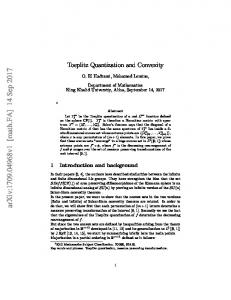
iii) Ali-Mikhail-Haq’s copula, with generator ψθ (t) = ln( 1−θ t + θ ), θ ∈ [−1, 1); iv) Clayton copula, with generator ψθ (t) = θ1 (t −θ − 1) , θ ∈ [−1, ∞)\{0}; v) Gumbel copula, with generator ψθ (t) = (− log(t))θ , θ ∈ [1, ∞). Following the procedures highlighted in e.g., [42] one can readily generate a scatter plot in order to illustrate the dependency structure induced by specific copulæ and observe that they are quite different. Since this is somewhat orbital to the current work, we have not included a concrete figure. We provide a brief illustration of several dependency structures for m = 2 in Figure 1 (e.g., [42] and references therein). This figure illustrates a scatter plot of u ∈ [0, 1]2 generated according to the joint distribution C.

(a) Gumbel(3)

(b) Gumbel(5)

(g) Frank(3)

(c) Clayton(1)

(h) Frank(5)

(d) Clayton(3)

(i) AMH(-1)

(l) Joe(3)

(e) Clayton(5)

(j) AMH(0)

(f) Frank(-1)

(k) AMH(0.9)

(m) Joe(5)

Figure 1. The dependency structure for several copulæ. Each point represents a randomly generated realization. Since the

marginal distributions of a copula are uniform, each random realization belongs to [0, 1]2 . The number in between parentheses is the parameter of the copula. The abbreviation AMH stands for Ali-Mikhail-Haq. In order to show that X(p) in (3b) is a convex set for a given copula C, we will make extensive use of generalized concavity and its properties. We will introduce notation and useful results in the following subsection. 2.2 Generalized concavity and its properties In order to define generalized concavity in a convenient way, the following function will be required. Definition 3. Let α ∈ [−∞, ∞] and mα : R+ × R+ × [0, 1] → R be defined as follows mα (a, b, λ ) = 0 if ab = 0,


for a > 0, b > 0, λ ∈ [0, 1]:  aλ b1−λ    max {a, b} mα (a, b, λ ) = min {a, b}    1 α (λ a + (1 − λ )bα ) α

if if if

α =0 α =∞ α = −∞ otherwise.

The following lemma, given in [12], will be used throughout this text. Lemma 1. ([12, Lemma 4.8]) Let mα be the mapping as defined in Definition 3. The mapping α 7→ mα is nondecreasing and continuous. We now provide the definition of generalized concavity: Definition 4. A non-negative function f defined on some convex set C ⊆ Rn is called α-concave (α ∈ [−∞, ∞]) if and only if for all x, y ∈ C, λ ∈ [0, 1]: f (λ x + (1 − λ )y) ≥ mα ( f (x), f (y), λ ),

(5)

where mα is as in Definition 3. ˜ for all α˜ ≤ α. A function f is 0-concave if Remark 1. If, for some α ∈ [−∞, ∞], f is α-concave, then it is also α-concave its logarithm is concave. This is usually referred to as log-concavity. For α 6= 0, α ∈ R, the function f is α-concave if either f α is concave for α > 0 or f α is convex for α < 0. In particular, if α = 1 then f is simply concave, and if α = −∞ then f is quasi-concave. For some further calculus rules with α-concavity we refer to Theorems 4.19–4.23 of [12]. We also recall the definition of generalized concavity for copulæ, [56]: Definition 5. Let γ ∈ R be given, and let the set D(γ) be defined as D(γ) = [0, 1]m for γ > 0, D(0) = (−∞, 0]m and D(γ) = [1, ∞)m for γ < 0. Let δ ∈ [−∞, ∞] be equally given. We call a copula C : [0, 1]m → [0, 1] δ -γ-concave if the mapping 1

u : D(γ) 7→ C(u γ ) is δ -concave, whenever γ 6= 0 and u : D(0) 7→ C(eu ) is δ -concave whenever γ = 0. In Definition 5 the generalized concavity properties need not hold on the full set D(γ), but only on a specific subset of it. It is therefore also useful to introduce the following local version of δ -γ-concavity for copula (see [56]). Definition 6. Let q ∈ (0, 1)m be some point and define the sets D(q, γ) as follows D(q, γ) = ∏m i=1 [qi , 1] for γ > 0, D(q, 0) = γ m m → [0, 1] δ -γ-q-concave if the mapping [log(q ), 0] and D(q, γ) = [1, q ] for γ < 0. We call a copula C : [0, 1] ∏m ∏ i i=1 i=1 i γ

1

u : D(q, γ) 7→ C(u γ ) is δ -concave, whenever γ 6= 0 and u : D(q, 0) 7→ C(eu ) is δ -concave whenever γ = 0. Remark 2. Notice that for δ = −∞ and γ = 1, i.e., −∞-1-concavity of a copula C : [0, 1]m → [0, 1] the notion of δ -γ-concavity is equivalent to ordinary quasi-concavity of the same function C on [0, 1]m . This property yields convexity of the level sets {u ∈ [0, 1]m : C(u) ≥ p}, for all p ∈ [0, 1] and conversely, as is well known.

3. Convexity statements: convexity of the nominal problem and the value function 3.1 Convexity of the nominal problem We now gather and extend some results given in [56] to establish convexity of the feasible set X(p) in (3b). Theorem 1. Let ξ ∈ Rm be a random vector with associated copula C, and let gi : Rn → R be functions such that P[ξ ≤ g(x)] = C(F1 (g1 (x)), ..., Fm (gm (x))), where Fi is the marginal distribution function of random variable ξ i , for i = 1, ..., m. Assume that, for any i = 1, ..., m, we can find αi ∈ R, such that the functions gi are αi -concave and a second set of parameters γi ∈ (−∞, ∞], bˆ i > 0 such that either one of the following conditions holds: 1 i) αi < 0 and z 7→ Fi (z αi ) is γi -concave on (0, bˆ αi i ] ii) αi = 0 and z 7→ Fi (exp z) is γi -concave on [log bˆ i , ∞)


1

iii) αi > 0 and z 7→ Fi (z αi ) is γi -concave on [bˆ αi i , ∞), ˆ where i ∈ {1, ..., m} is arbitrary. If the copula is either δ -γ-concave or δ -γ-F(b)-concave for γ ≤ γi ≤ ∞, i = 1, ..., m, it holds that a) the set M(p) := {x ∈ Rn : P[ξ ≤ g(x)] ≥ p} is convex for all p > pM := maxi=1,...,m Fi (bˆ i ); b) if, in addition, each individual distribution function Fi , i = 1, ..., m is strictly increasing, then convexity can moreover be derived for all p ≥ pM ; c) if αi ≥ 0 and Fi is γi -concave everywhere, i = 1, ..., m, then the set M(p) is convex for all p ∈ [0, 1]. We now weaken the assumption on gi : assume that there exists a vector b ∈ Rm , such that gi is αi -concave, on the level sets D := {x ∈ Rn : gi (x) ≥ bi , ∀ i = 1, . . . , m} for αi ∈ R. Moreover, the marginals Fi satisfy once again either one of the conditions i)-iii), but they are not necessarily strictly increasing. By defining p∗ := C(F1 (b1 ), . . . , Fm (bm )), it holds that ˆ then the set M(p) ∩ D is convex for all p ≥ p∗ ; d) if b ≥ b, e) if ì ≥ max{bi , bˆ i }, i = 1, . . . , m, then the feasible set X(p) in (3b) is a convex set for all p ≥ p∗ . Proof. Items a), b) and c) are given in [56, Theorem 4.1]. Item d) follows from [56, Theorem 4.2]. Identity (2) and inequality ` ≥ b provide the inclusion X(p) ⊂ M(p) ∩ D. Hence, item e) follows from item d). Corollary 1. In the setting of Theorem 1, assume that αi = 1 and that Fi is γi -concave everywhere, where γi ∈ (−∞, ∞] for all i = 1, . . . , m. If the copula is δ − γ-concave, the feasible set X(p) in (3b) is convex for all p ∈ [0, 1] regardless of ì ∈ [−∞, ∞), i = 1, . . . , m. Proof. Note that X(p) = M(p) ∩ {x ∈ Rn : gi (x) ≥ ì , ∀ i = 1, . . . , m}. Then the result follows from concavity of gi (which is equivalent to αi -concavity for αi = 1) and item c) above. Note that the extension of the results of [56] contained in Theorem 1 resides in making explicit that it is sufficient for gi to be generalized concave on specific sets only. An important assumption in Theorem 1 is that the considered copula: C : [0, 1]m → [0, 1] needs to be δ -γ-concave. Next, we show that all Archimedean copulæ belong to the class of δ -γ-concave copulæ and, hence, provide eventually convexity of the feasible set X(p) given in (3b). Theorem 2. Let C : [0, 1]m → [0, 1] be an Archimedean copula, and ψ : (0, 1] → [0, ∞) be its generator. Then C is a −∞-1concave copula, i.e., a quasi-concave copula. Proof. We just need to show that the level sets M(p) := {u ∈ [0, 1]m : C(u) ≥ p} are convex for all p ∈ [0, 1]. To this end, let λ , p ∈ [0, 1] be arbitrary and u1 , u2 ∈ M(p) be given. Since ψ [−1] (ψ(u)) = u, and ψ is decreasing by definition, the inequality C(ui ) ≥ p is equivalent to ∑mj=1 ψ(uij ) ≤ ψ(p), i = 1, 2. By defining uλ = λ u1 + (1 − λ )u2 and convexity of ψ we obtain m

ψ(C(uλ )) =

∑ ψ(uλj ) ≤ λ

j=1

m

m

∑ ψ(u1j ) + (1 − λ ) ∑ ψ(u2j )

j=1

(6)

j=1

≤ λ ψ(p) + (1 − λ )ψ(p) = ψ(p) . Since ψ is the generator of an Archimedean copula, Theorem 2.2 in [36] ensures that ψ [−1] is m-monotone. In particular, ψ [−1] is a non-increasing function. Therefore, the inequality C(uλ ) ≥ p follows from applying ψ [−1] in (6). We have thus shown that uλ ∈ M(p), establishing the stated result. Remark 3. We care to note that stronger generalized concavity properties are known for the Clayton copula. Indeed, it is δ -0 concave for specific δ values depending on the parameter of its generator (see [56]). Similarly, the Gumbel, independent and maximum copulæ are 0-0-concave as shown in [25]. 3.2 Convexity of the value function in generalized Benders decomposition If X(p) in (3b) is a nonempty and convex set, and f is a convex function, then under a Slater type assumption, any KKT point for problem (3) is also an optimal solution. Note that the Slater assumption, i.e., the existence of x such that (1) is satisfied strictly is a mild assumption (for instance also needed for stability results [23]). If, moreover, all the involved functions are differentiable, then the task of solving (3) can be carried out by general purpose solvers for nonlinear and differentiable optimization. There are, however, situations in which more specialized algorithms are preferable for solving problem (3) through suitable reformulations. For instance, when the considered copula is difficult to evaluate, as discussed in § 5.1.4 below. Another situation arises when some or all constraints gi are nonsmooth, but suitable reformulations exist that allow their handling with specialized algorithms. This case is addressed in the first part of Section 5.


The use of additional variables frequently plays an important role in the quest of efficiently solving optimization problems. Indeed, since the marginal distribution function Fi is monotonically nondecreasing, the constraint gi (x) ≥ ì in (3b) is equivalent to Fi (gi (x)) ≥ Fi (ì ). Therefore, by adding the extra variables u ∈ [0, 1]m problem (3) is equivalent, in terms of optimal value and feasible region for x, to  min f (x)     (x,u)∈X×[0,1]m s.t. C(u) ≥p (7)  F (g (x)) ≥ ui , i = 1, . . . , m  i i   ui ≥ Fi (ì ), i = 1, . . . , m . The value function v : [0, 1]m → R ∪ {∞} defined in (4b) is thus obtained by splitting variables x and u from the above problem, and representing the constraint Fi (gi (x)) ≥ ui by gi (x) ≥ Fi−1 (ui ), avoiding the need of computing derivatives for the (very often implicit) function Fi . As already mentioned in the introduction, under appropriate assumptions on functions f and gi , i = 1, . . . , m, problem (4b) can be easily solved. For instance, if f and all gi are linear (respectively concave quadratic) functions, (4b) is a linear (respectively convex conic) programming problem. The value function v allows us to split problem (7) into two subproblems: the slave subproblem (4b) and the master problem (4a). The relation between formulations (3) and (4) is established by the following result, whose elementary proof is omitted. Lemma 2. Assume that problem (3) admits an optimal solution. Then problem (4) also admits an optimal solution and both optimal values are identical. Moreover, if u∗ is optimal for (4a), and x∗ optimal for problem (4b), in which u = u∗ , then x∗ is optimal for (3). Since C is a copula we cannot expect C to be concave in general (see for example Theorem 2). Still C may have generalized concavity properties such as δ -γ-concavity (Definition 5). Consequently, the feasible set in (4a) can not be properly approximated by using first-order linearizations of C, a standard procedure in convex (nonsmooth) optimization. If C happens to be δ -γ-concave for some γ ≤ 1, then the feasible set in problem (4a) is a convex set. We recall here that (see [56, Lemma 3.5]) δ -γ-concavity of a copula implies δ -α-concavity of the same copula for all α ≥ γ. If C fails to be δ -γ-concave, we have nonetheless split the non-convexity induced by the copula from the inherent convexity structure in v. Convexity of function v is ensured by the following result. Lemma 3. Let f : Rn → R be a real-valued and convex function. Assume, moreover that, for each i = 1, . . . , m, we can find αi ∈ R such that the functions gi are αi -concave on level sets {x ∈ R : gi (x) ≥ bi }, and a second set of parameters γi ∈ [1, ∞], bˆ i > 0 satisfying either one of the conditions i), ii) or iii) in Theorem 1. Moreover, suppose that ì ≥ max{bi , bˆ i }, i = 1, . . . , m. Then v defined in (4b) is a convex function on the set {u ∈ [0, 1]m : ui ≥ Fi (ì ), i = 1, . . . , m}. For any given u ∈ Dom(v), suppose that problem (4b) admits optimal Lagrange multipliers sui associated with the constraints Fi (gi (x)) ≥ ui , i = 1, . . . , m. Then, the vector su belongs to the subdifferential of v at the point u, i.e., su ∈ ∂ v(u). Proof. Let u1 , u2 ∈ {u ∈ [0, 1]m : ui ≥ Fi (ì ), i = 1, . . . , m} ∩ Dom(v) be arbitrary points, and x1 , x2 ∈ X be optimal solutions of problem (4b), with u replaced by u1 and u2 , respectively. Pick λ ∈ (0, 1) arbitrarily and define uλ = λ u1 + (1 − λ )u2 ; define xλ similarly. It follows by convexity of the polyhedral set X that xλ ∈ X. We now make a case distinction to show that Fi (gi (xλ )) ≥ uλ for all i = 1, . . . , m. First notice that Fi (gi (x j )) ≥ uij from (4b) and uij ≥ Fi (ì ) from (4a) yield gi (x j ) ≥ ì for j = 1, 2. Now, remember that ì ≥ bˆ i > 0 (thus the bˆ i -dependent intervals in items i)-iii) become smaller for bˆ i replaced by ì ) and fix i = 1, ..., m for the moment to consider the following cases: Case 1. Suppose that αi < 0. In this case, gi (x j )αi ≤ `αi i for j = 1, 2. Hence, `αi i ≥ max {gi (x1 )αi , gi (x2 )αi } ≥ λ gi (x1 )αi + (1 − λ )gi (x2 )αi . Case 2. Suppose that αi > 0. In this case, gi (x j )α ≥ `αi i for j = 1, 2. Hence, `αi i ≤ min {gi (x1 )αi , gi (x2 )αi } ≤ λ gi (x1 )αi + (1 − λ )gi (x2 )αi . Case 3. Since the log function is increasing, we have that log(gi (x j )) ≥ log(ì ) for j = 1, 2. Hence, log(ì ) ≤ min {log(gi (x1 )), log(gi (x2 ))} ≤ λ log(gi (x1 )) + (1 − λ ) log(gi (x2 )). By using the notation mα (·, ·, λ ) of Definition 3, the three cases above correspond to ì ≤ mαi (gi (x1 ), gi (x2 ), λ ) ,


where case 3 is related to αi = 0. Since gi is αi -concave on the level set {x ∈ Rn : gi (x) ≥ bi } (and thus on {x ∈ Rn : gi (x) ≥ ì }), it follows from Definition 4 that ì ≤ mαi (gi (x1 ), gi (x2 ), λ ) ≤ gi (xλ ). From monotonicity of the probability distribution function Fi , and Cases 1 and 2 above, we obtain Fi (gi (xλ )) ≥ Fi (mαi (gi (x1 ), gi (x2 ), λ )) 1

1

= Fi ((λ gi (x1 )αi + (1 − λ )gi (x2 )αi ) αi ) = Fi (z α i ), for z = λ gi (x1 )αi + (1 − λ )gi (x2 )αi satisfying 0 < z

≤ `αi i

if αi < 0 and z

(8) ≥ `αi i

if αi > 0. In case 3 it follows that

Fi (gi (xλ )) ≥ Fi (m0 (gi (x1 ), gi (x2 ), λ )) = Fi (exp (λ log gi (x1 ) + (1 − λ ) log gi (x2 ))) = Fi (exp(z)),

(9)

for z = λ log gi (x1 ) + (1 − λ ) log gi (x2 ) satisfying z ≥ log(ì ) if αi = 0. The mappings Fi are γi -concave by assumption on a specific bˆ i -dependent domain given in conditions i), ii) or iii) of Theorem 1. Since we have shown in (8) and (9) that z belongs to this domain (because ì ≥ bˆ i > 0), we can apply γi -concavity and obtain: Fi (gi (xλ )) ≥ mγi (Fi (gi (x1 )), Fi (gi (x2 )), λ ). Since γi ≥ 1 and m1 is monotonic in its first two arguments (Lemma 1), the latter inequality gives Fi (gi (xλ )) ≥ mγi (Fi (gi (x1 )), Fi (gi (x2 )), λ ) ≥ m1 (Fi (gi (x1 )), Fi (gi (x2 )), λ ) ≥ m1 (u1 , u2 , λ ) = uλ . Consequently

xλ

is feasible for problem (4b) with u replaced by

uλ ,

(10)

which in turn implies by convexity of f that

v(uλ ) ≤ f (xλ ) ≤ λ f (x1 ) + (1 − λ ) f (x2 ) = λ v(u1 ) + (1 − λ )v(u2 ) . The above relation holds trivially if at least u1 or u2 does not belong to Dom(v). Hence, we have shown that v is indeed a convex function on {u ∈ [0, 1]m : ui ≥ Fi (ì ), i = 1, . . . , m}. Let u ∈ Dom(v) be given. Since (4b) is a convex programming problem, the remainder of the proof follows from [45, Theorem 4.26], which shows that any optimal Lagrange multiplier su is a subgradient of v at u. Notice that there is a gap between the convexity results of Theorem 1 and those of Lemma 3. The former allows for the parameters γi ∈ (−∞, ∞], whereas the latter requires γi ≥ 1. This gap can actually be filled by appropriately redefining v as indicated below: Corollary 2. Let D(γ) be as in Definition 5. Under the assumptions of Lemma 3 assume the existence of a γ ∈ (−∞, ∞) such that γi ≥ γ for all i = 1, ..., m and that v : D(γ) → R ∪ {∞} given in (4b) is (re-)defined as follows: 1

v(u) = min f (x) s.t. Fi (gi (x)) ≥ uiγ , i = 1, . . . , m,

(11a)

x∈X

when γ 6= 0 and v(u) = min f (x) s.t. Fi (gi (x)) ≥ exp(ui ), i = 1, . . . , m,

(11b)

x∈X

1

when γ = 0. Then v is a convex function on the set {u ∈ D(γ) : uiγ ≥ Fi (ì ), i = 1, ..., m} (γ 6= 0) or {u ∈ D(γ) : exp(ui ) ≥ Fi (ì ), i = 1, ..., m} (γ 6= 0). Proof. The proof of Lemma 3 can be carried over verbatim up until (10), when we notice that for γ 6= 0, combining Fi (gi (x)) ≥ 1

1

uiγ with uiγ ≥ Fi (ì ) allows us to establish gi (x) ≥ ì . The case γ = 0 follows likewise. We now establish the equivalent of (10). For the case γ 6= 0, we can substitute here: Fi (gi (xλ )) ≥ mγi (Fi (gi (x1 )), Fi (gi (x2 )), λ ) ≥ mγ (Fi (gi (x1 )), Fi (gi (x2 )), λ ) 1

1

1

≥ mγ (u1γ , u2γ , λ ) = (uλ ) γ , and when γ = 0, Fi (gi (xλ )) ≥ mγi (Fi (gi (x1 )), Fi (gi (x2 )), λ ) λ

≥ m0 (Fi (gi (x1 )), Fi (gi (x2 )), λ ) ≥ m0 (eu1 , eu2 , λ ) = eu . The remainder of the proof can then also be copied verbatim.


Since u ∈ [0, 1]m can be arbitrary, problem (4b) may be infeasible. In order to deal with this, we consider the following auxiliary problem: ( kzk1 min x∈X,z∈Rm + f(u) := (12) s.t. Fi (gi (x) + zi ) ≥ ui , i = 1, . . . , m Since X 6= 0, / problem (12) is feasible for all u ∈ [0, 1]m . Therefore, f is a finite valued function: f : [0, 1]m → R+ . Moreover, f(u) = 0 if and only if the feasible set of problem (4b) is nonempty. Lemma 4. Under the assumptions of Lemma 3, function f given in (12) is convex on {u ∈ [0, 1]m : ui ≥ Fi (ì ), i = 1, . . . , m}. Moreover for any given u ∈ [0, 1]m , any optimal Lagrange multiplier sui associated to the constraints Fi (gi (x) + zi ) ≥ ui , i = 1, . . . , m, satisfies su ∈ ∂ f(u). The linearization f(u) + hsu , u˜ − ui ≤ 0,

(13)

is a feasibility cut for problem (4a). ˜ for all u˜ feasible for (4a). Proof. The proof is analogue to Lemma 3. Therefore, by convexity of f, f(u) + hsu , u˜ − ui ≤ f(u) Since we wish to exclude points u that yields f(u) > 0, inequality (13) is indeed a feasibility cut.

4. Algorithm: regularized GBD with an interpolation step We now investigate algorithms for solving problem (3) through formulation (4). In view of Theorem 1 and Lemma 3 we will assume throughout this section that v : Rm → R ∪ ∞ in (4b) is an extended real-valued and convex function, and the feasible set of (4a) is nonempty and convex for a large enough p ∈ (0, 1]. We are, however, assuming that C satisfies only generalized concavity assumptions. If the domain of v contains the feasible set of problem (4a), then we can solve (4) (and therefore problem (3)) by applying the supporting hyperplane algorithm proposed in [62] to the following reformulated problem: min

y≤y≤y, u∈[0,1]m

y

s.t.

v(u) ≤ y, C(u) ≥ p, ui ≥ Fi (ì ), i = 1, . . . , m ,

where y and y are properly chosen bounds satisfying y ≤ vmin ≤ y. In the application of interest, the domain of v does not contain, in general, the m-dimensional unit box and therefore feasibility cuts must be added to the above problem. As a result, [62] cannot be directly applied to this reformulation (the algorithm in [62] is suitable for real-valued functions, only). Even endowing the supporting hyperplane algorithm of Veinott with means to handle extended real-valued functions the resulting (new) algorithm is not very appealing: supporting hyperplane method possesses slow convergence and requires many function evaluations for solving the problem. Since function v in (26) is costly, we would like to employ a method for solving (4a) that requires as few function evaluations as possible. In the quest of efficiently solving (4a), we thus propose a new variant of level bundle methods [31] for nonsmooth optimization problems whose objective function is convex but can assume the value infinity, and wherein the nonlinear constraint mappings satisfy only generalized concavity assumptions. To the best of our knowledge, the proposed optimization method is the first bundle algorithm with global convergence guarantees for such an optimization setting. The full algorithm is described in § 4.2, but first we present some key ingredients. 4.1 Ingredients: cutting-plane models Given a sequence of generated trial points u˜1 , u˜2 , . . . , u˜k , we will split the index set {1, . . . , k} into two subsets: the optimality index set Øk gathering indices j such that v(u˜ j ) < ∞, and the feasibility index set Fk gathering indices j such that f(u˜ j ) > 0. We thus have that Øk ∩ Fk = 0/ and Øk ∪ Fk = {1, . . . , k}. Accordingly, we define the cutting-plane models for function v and f, respectively: n D Eo n D Eo j j j j m j j vm (u) := max v( u ˜ ) + s , u − u ˜ , f (u) := max f( u ˜ ) + s , u − u ˜ . k k u˜ u˜ j∈Fk

j∈Øk

vm k

fm k

Since v and f are convex functions, the models and approximate, respectively, v and f from below. As C is not concave, we cannot approximate C by using first-order linearizations of the type C(u) + h∇C(u), · − ui without cutting-off the set M(p) = {u ∈ [0, 1]m : C(u) ≥ p} .

(14)

However, since this latter set is convex (e.g., Theorem 1), we can approximate M(p) by using tangent directions, as shown by the following classic result (e.g., [26, Chapter III]).


Lemma 5. Let C : [0, 1]m → [0, 1] be a continuously differentiable copula such that M(p) given in (14) is a convex set for a given p ∈ [0, 1]. Then for any u˜ ∈ [0, 1]m such that C(u) ˜ = p, the inequality h∇C(u), ˜ u − ui ˜ ≥ 0 is a supporting hyperplane for M(p). Moreover, if ∇C(u) ˜ 6= 0 and if uin is a point in the interior of M(p), then, h∇C(u), ˜ uin − ui ˜ > 0. Remark 4. The existence of a point uin in the interior of M(p), defined in (14), is not a restrictive assumption. Indeed, for Archimeadean copulæ such a point uin can be easily computed: let p ∈ (0, 1) and ϕθ (the copula generator function) be given ϕ ( p+1 ) and 1 be the vector of ones in Rm . Then uin defined as uin := 1ϕθ−1 θ m2 is readily seen to belong to interior of M(p). Note that by taking uin sufficiently large enough (close to 1), one can ensure that uin i > Fi (ì ) holds as well. Conditions on C that ensure the property ∇C(u) ˜ 6= 0 for C(u) ˜ = p > 0 are studied in Appendix A. Such conditions hold whenever C is an Archimedean copula. Having the cutting-plane information at iteration k, let vk+1 low be the optimal value of the following linear programming problem:  min vm  k (u)   u m s.t. f k (u) ≤ 0

vk+1 low := j ), u ≥ ∇C(u˜ j ), u˜ j , i) = p  ∇C( u ˜ j ∈ i ≤ k : C( u ˜   u ∈ [0, 1]m , ui ≥ Fi (ì ), i = 1, . . . , m .

(15)

In view of Lemma 5 problem (15) is an outer-approximation of problem (4a). As a result, vk+1 the optimal low is a lower boundfor k and u˜k value of (4a): vk+1 ≤ v for all k = 1, 2, . . .. Algorithm 1 given below generates two sequences of iterates: u min low both satisfying the last two constraints in (15), where the last sequence satisfies also C(u˜k ) ≥ p for all k. Since u˜k is a feasible point, v(u˜k ) is an upper bound for the optimal value of problem (4a): vmin ≤ v(u˜k ) for all k = 1, 2, . . .. An optimality measure for problem (4a) is, therefore, the gap ∆k+1 := min v(u˜ j ) − vk+1 low . j∈Øk

(16)

Indeed, if ∆k+1 ≤ ε for some tolerance ε > 0, we have that j ε ≥ min v(u˜ j ) − vk+1 low ≥ min v(u˜ ) − vmin ≥ 0. j∈Øk

j∈Øk

(17)

(If the index i is defined as i := arg min j∈Øk v(u˜ j ), then u˜i is ε-optimal for (4a) since v(u˜i ) ≤ vmin + ε.) We now explain how our algorithm defines the two sequences of iterates uk and u˜k . In order to do that, we select a parameter κ ∈ (0, 1) and a stability center uˆk feasible for problem (4a). The sequence uk is generated by solving, at iteration k, the following problem: 

2  min u − uˆk   u    s.t. vm (u) ≤ vklow + κ∆k k f m (u) ≤ 0

k    ∇C( u˜ j ), u ≥ ∇C(u˜ j ), u˜ j , j ∈ i ≤ k : C(u˜i ) = p    u ∈ [0, 1]m , ui ≥ Fi (ì ), i = 1, . . . , m , We propose to set uˆ0 := uin , kref := 1 and update the stability center according to the rule k+1 u if ∆k+1 ≤ (1 − κ)∆kref (in this case set kref ← k + 1) uˆk+1 ← uˆk if ∆k+1 > (1 − κ)∆kref .

(18)

(19)

k k k in However, other rules for updating the stability center are possible. For instance, we can set uˆ = u for all k or, simply, uˆ = u in k for all k. Let u as in Lemma 5 be given, then the sequence of feasible points u˜ is obtained by defining

u˜k = uin + λ k (uk − uin ) ,

(20)

where λ k ∈ (0, 1] is the largest number such that C(u˜k ) ≥ p. Accordingly, u˜k = uk whenever C(uk ) ≥ p (i.e., λ k = 1), and C(u˜k ) = p if C(uk ) < p. In this latter case, continuity of C ensures that u˜k as in (20) can be computed by employing a bisection procedure on the interval [0, 1].


4.2 A regularized supporting hyperplane algorithm We now present our algorithm, which we will refer to as RSHM in the sequel. Algorithm 1. A REGULARIZED SUPPORTING HYPERPLANE ALGORITHM Step 0 (Initialization) Let uin be as in Lemma 5. Set Ø0 = F0 = 0, / ∆1 = ∞, u˜1 = uin , k = 1 and choose ε > 0 and κ ∈ (0, 1). Step 1 (Stopping Test) If ∆k ≤ ε, stop. Step 2 (Oracle v) Try to compute v(u˜k ) and sku˜ ∈ ∂ v(u˜k ). If problem (4b) is infeasible, set Øk ← Øk−1 and go to Step 3. Otherwise, set Øk ← Øk−1 ∪ {k}, Fk ← Fk−1 and go to Step 4. Step 3 (Oracle f) Compute f(u˜k ), sku˜ ∈ ∂ f(u˜k ) and set Fk ← Fk−1 ∪ {k}. k+1 by solving the master problem (18). Step 4 (Primal Step) Compute vk+1 low by solving the LP problem (15) and u k+1 k+1 k+1 Step 5 (Bisection) If C(u ) < p, compute u˜ as in (20) and ∇C(u˜ ). Otherwise, set u˜k+1 = uk+1 . Step 6 (Loop) Compute ∆k+1 as in (16) and obtain uˆk+1 as in (19) (or another suitable rule). Set k ← k + 1 and return to Step 1.

The case in which either Øk or Fk is an empty set deserves comments: (i) if Øk = 0, / then (15) must be interpreted as the problem of finding a point uk+1 in the feasible set defined in (15). In this case, vk+1 should be defined as −∞; (ii) if Fk = 0, / low then fm is meaningless, and it should be removed from (15) and (18). Since at each iteration the algorithm adds more constraints k in problem (15) (because either Øk or Fk is enlarged), we conclude that the sequence {vklow }k is non-decreasing. The original level method [31] was designed to solve optimization problems with convex objective and constraint functions (concave functions if we are thinking of constraints of the type C(u) ≥ p). Each iteration of the level method in [31] involves solving two optimization subproblems; first a linear program to compute the level parameter vklow + κ∆k , and then a projection problem to define a new iterate. This is also the strategy adopted by Algorithm 1 that successively solves both subproblems (15) and (18) at each iteration of the algorithm. However, solving (15) to define a lower bound vk+1 low is optional. In fact, we can let the lower bound fixed along some iterations until the algorithm identifies that the master problem (18) is infeasible. In this case, k+1 k k the lower bound must be increased: the most common rule is to set vk+1 low = vlow + κ∆k if (18) is infeasible, and vlow = vlow k 0 otherwise. This rule ensures that, for any k > 0, vlow is a lower bound for the optimal value of (4a) as long as vlow satisfies v0low ≤ vmin ; see [57, Lemma 2]. 4.3 Convergence analysis In order to establish convergence we will need the following auxiliary result. Lemma 6. Consider Algorithm 1 and assume that ∇C(·) is continuous on [0, 1]m and 0 6= ∇C(u) for all u ∈ [0, 1]m suchthat C(u) = p. Assume that the algorithm generates an infinite sequence of iterates. Let u˜ be a cluster point of the sequence u˜k . Then, there exists an index set K ⊆ N such that limk∈K uk = u˜ = limk∈K u˜k . Proof. Since uk k≥0 , u˜k k≥0 ⊂ [0, 1]m and λ k k≥0 ⊂ (0, 1] are bounded sequences, there exist convergent subsequences indexed by kl satisfying liml (ukl , u˜kl , λ kl ) = (u, ¯ u, ˜ λ¯ ). If C(u) ˜ > p, then continuity of C, together with Step 5 of the algorithm k k l l entails that u = u˜ for l sufficiently large and hence u ¯ = u.We ˜ may therefore assume that C(u) ˜ = p. It follows from (20) that if λ¯ = 1, then the cluster point u¯ of ukl coincide with u, ˜ and the stated result follows for such a K. In what follows we will assume that λ kl < 1 for all l ≥ l¯ to show that λ¯ = 1 (if such index l¯ does not exist, then we can construct an infinite subsequence 0 λ kl = 1 for all kl0 and the result λ¯ = 1 holds trivially). First, take t ∈ (0, 1) and define u(t) := u˜kl + t(ukl − u˜kl ) = uin + [t + (1 − t)λ kl ](ukl − uin ). Since λ kl is the largest value such that C(u˜kl ) ≥ p, it follows from the inequality t + (1 − t)λ kl > λ kl that C(u(t)) < p ≤ C(u˜kl ) for all t ∈ (0, 1). Therefore, ukl − u˜kl is a descent direction for C at u˜kl , and thus ∇C(u˜kl ), ukl − u˜kl ≤ 0.

Moreover, it follows from (15) that ∇C(u˜kl ), ukl+1 ≥ ∇C(u˜kl ), u˜kl . By gathering these two last inequalities we have D E D E D E ∇C(u˜kl ), ukl+1 ≥ ∇C(u˜kl ), u˜kl ≥ ∇C(u˜kl ), ukl . Passing to the limit when l goes to infinity and recalling continuity of ∇C(·) we get that h∇C(u), ˜ ui ¯ = h∇C(u), ˜ ui, ˜ and from (20), u˜ = λ¯ u¯ + (1 − λ¯ )uin . These two inequalities yield: (1 − λ¯ ) h∇C(u), ˜ ui ˜ = (1 − λ¯ ) h∇C(u), ˜ uin i . Since h∇C(u), ˜ uin − ui ˜ >0 ¯ from Lemma 5, we conclude that λ = 1, and the result follows. Convergence of Algorithm 1 is given in the following theorem. Theorem 3. Under the assumptions of Lemma 3, suppose in addition that all subgradients of v generated by the oracle in Step 2 of Algorithm 1 are uniformly bounded, ∇C(·) is continuous on [0, 1]m and 0 6= ∇C(u) for all u ∈ [0, 1]m such that C(u) = p. Moreover, suppose that ε = 0 and that the algorithm produces infinitely many optimality cuts whose indices are gathered in the index set Ø. Then, any cluster point u˜ of the sequence u˜k k∈Ø generated by Algorithm 1 is a solution to problem (4a).


Proof. Under the assumptions of Lemma 3, function v defined in (4b) is a convex mapping, and ∆k+1 defined in (16) is indeed an optimality gap. Therefore, in order to D obtain the stated E result we just need to show, from (17), that ∆k → 0. kl i+1 k k l l Subproblem (18) provides v(u˜ ) + su˜ , u − u˜ ≤ vi+1 low + κ∆i+1 for all kl ∈ Ø and i ≥ kl . Therefore,

D E

kl kl kl i+1 i+1 − u ≤ Λ u ˜ − u (21) (1 − κ)∆i+1 ≤ v(u˜kl ) − vi+1 − κ∆ ≤ s , u ˜

. i+1 low u˜

where Λ > 0 is a constant such that sku˜ ≤ Λ for all k ∈ Ø. Since u˜k k∈Ø is bounded, it has a cluster point u. ˜ It follows from Lemma 6 that there exists a subsequence with indice kl ∈ Ø such that liml→∞ u˜kl = liml→∞ ukl = u. ˜ In order to show that u˜ solves (4a), recall that κ ∈ (0, 1), take i = kl+1 in (21), and pass to the limit with l → ∞. Since v is a convex function on {u ∈ [0, 1]m : ui ≥ Fi (ì ), i = 1, . . . , m}, its subdifferential is compact on ri(Dom(v)) ∩ {u ∈ [0, 1]m : ui ≥ Fi (ì ), i = 1, . . . , m}. Therefore, for points u in the latter set the constant Λ > 0 in Theorem 3 is ensured. However, for points u ∈ Dom(v) \ ri(Dom(v)) we request the oracle to return bounded subgradients, i.e., bounded Lagrange multipliers for problem (4b). The assumption that ∇C(·) is continuous and differs from zero for all u ∈ [0, 1]m such ∇C(u) = p is satisfied, ¯ only feasibility cuts are for instance, for all Archimedean copulæ; see Corollary 4 in appendix A. If, after a certain iteration k, generated, it can be shown that limk f(u˜k ) = 0. Hence, any cluster point of u˜ of {u˜k } belongs to the domain of v. We finalize this section by mentioning that the given convergence analysis does not require any assumption on the norm k·k in (18). If the

2

objective function u − u˜k is replaced with u − u˜k 1 or u − u˜k ∞ (i.e., `1 or `∞ norms), then the resulting master problem becomes a linear programming problem. This is an interesting feature for dealing with large-scale optimization problems, whose quadratic master solution can be expensive. The convergence speed may be reduced by this change in stabilization. However, this may largely be compensated by a gain in resolution speed because the master problem is less expensive [2, 17, 18].

5. Test problems and numerical experiments We now focus on the numerical solution of problem (3). The task of choosing a suitable copula that models the dependency among the random variables {ξ 1 , . . . , ξ m } is beyond the scope of this work and will not be discussed here. The M ATLAB sources and test-problem generator (as well as many copulæ) used in Section 5.1 below are publicly available on the second author’s web page: www.oliveira.mat.br/solvers. 5.1 Approximation of a chance-constrained problem with random technology matrix In this subsection we consider the following special case of problem (3) where the mappings gi in (3b) are given by ai − µ T x gi (x) = p i , x T Σi x

(22)

with given vectors µi ∈ Rn and symmetric positive definite matrices Σi ∈ Rn×n for all i = 1, . . . , m. These mappings satisfy some generalized concavity assumptions, as stated in the following lemma. Lemma 7 ((see [6]) ). Let a > 0 be given, µ ∈ Rn and Σ be an n × n positive definite matrix. Define the mapping g : D → R+ ∪ {∞} as: ( Tx a−µ √ if x 6= 0 xT Σx g(x) = (23) ∞ else, where D is the set D = x ∈ Rn : µ T x ≤ a . This mapping is (−r)-concave on the set {x ∈ D : g(x) > b(r)} , with b(r) :=

1 r+1 (λmin )− 2 kµk r−1

for all r ∈ (1, 3], where λmin > 0 is the smallest eigenvalue of the positive definite matrix Σ. Here we use the convention

(24) 1 ∞

= 0.

The above lemma is an improvement on [24] and a similar result appears in [6]. We provide a complete proof in the Appendix C as the one in [6] does not provide the computational details and we need to append r ≤ 3 for a key estimate as well as a > 0 and an appropriate handling of ∞ (i.e., x = 0). Given gi in (22), we assume that each component ξ i of the random vector ξ is a standard Gaussian random variable, i.e., ξ i ∼ N (0, 1) for all i = 1, . . . , m. Sklar’s Theorem ensures that there exists a suitable copula C such that the probability P[ξ ≤ g(x)] can be written as P[ξ ≤ g(x)] = P[ξ i ≤ gi (x), i = 1, ..., m] = C(Φ(g1 (x)), . . . , Φ(gm (x))) ,

(25)


where Φ (= Fi ) is the standard Gaussian cumulative distribution function. For instance, if the random variables {ξ 1 , . . . , ξ m } are mutually independent, then C above is the product (or independent) copula C(u) = Πm i=1 ui . In the dependent case, other copulæ must be used instead. Under these assumptions, problem (4b) defining function v(u) can be written as: v(u) = min x∈X

f (x)

s.t.

p µiT x + Φ−1 (ui ) xT Σi x ≤ ai , i = 1, . . . , m .

(26)

Consequently, if f is linear or quadratic convex, then the above problem is a convex conic optimization problem, and can be efficiently solved by standard methods. Remark 5. Consider the specific instance of problem (3) with constraint mappings (22) and structure (25). Item e) in Theorem 1 requires that ì ≥ bi , i = 1, . . . , m. Since bi = b(r) defined in (24) is positive, it follows that when u ∈ [0, 1]m is feasible p for (4a), then ui ≥ Fi (ì ) > Fi (0) = 12 . In this case Φ−1 (ui ) > 0 and the constraints in (26) reads as µiT x − ai ≤ −Φ−1 (ui ) xT Σi x < 0 for all x 6= 0. Moreover, by assuming that each component ai is strictly positive the nonlinear constraints in (26) are also satisfied for x = 0. Motivation. The motivation for this specific form of the mappings gi and ξ i comes from the following special form of constraint mapping P[ω T i x ≤ ai , i = 1, ..., m] ≥ p,

(27)

T where each ω i ∼ N (µ i , Σi ) follows a multi-variate Gaussian distribution. For each i = 1, ..., m, the following holds: P[ω i x ≤ a −µ T x ai ] = P ξ i ≤ √i T i = P[ξ i ≤ gi (x)]. Let ω be the m × n matrix stacking the m rows following distribution ω i . It is readily

x Σi x

observed that η(x) := ωx ∈ Rm is also a Gaussian random vector with x dependent mean of which the ith component equals µiT x and also with x dependent Covariance matrix Θ(x). For any i, j = 1, ..., m, one can show that Θi j (x) = xT Σi j x, where Σi j is ˜ the covariance matrix between rows i and j respectively and Σii = Σi . Now (27) is equivalent to P[η(x) ≤ g(x)] ≥ p, where ˜ g : Rn → Rm contains as i-th component the mapping gi given in (22), and η(x) is a centered multivariate Gaussian random i jx ˜ ˜ i j (x) = √ xT Σ√ variable with correlation matrix Θ(x) having components: Θ . Therefore, (25) considerably simplifies the T T x Σi x

x Σ jx

dependency structure in (27), already by removing the dependency on x in it. Still, dependency can be introduced through the choice of an x-independent Copula and we believe this to be worthwhile. It is clear that (25) fits the assumptions of this work. Moreover from the viewpoint of (27), defining g(0) = ∞ is natural. Indeed, when a > 0, it is readily seen in (27) that x = 0 is feasible for all p ∈ [0, 1]. By including x = 0 in the definition of g in this manner, it also belongs to the level set (24) and to the feasible set in (26), again regardless of p. 5.1.1 The problem, solvers, and instances for numerical experiments

From now on we focus on problem (3) whose objective function f is linear and constraints gi , i = 1, . . . , m, are given in (22). The problem data µi ∈ Rn , Σi ∈ Rn×n , ai ∈ R, i = 1, . . . , m and f (x) = cT x, with c ∈ Rn were generated randomly by using three different seeds for the random number generator. Vector c defining the linear function f was drawn from the sparse Gaussian distribution with mean equal to zero and variance equal to 300, i.e., N (0, 300). The vectors µi , i = 1, . . . , m, were defined by µi = 101√n Vi , where each coordinate of vector Vi ∈ Rn was randomly drawn from N (0, 1). Each matrix Σi was generated by using the Matlab function gallery(’randcorr’,n). Numbers ai were defined by the following rule, with 1 the vector of ones p m > −1 > in R : ai = µi 1 + Φ (0.55) 1 Σi 1 . In our implementation we make sure that the randomly generated data yields ai ≥oδ , n for i = 1, . . . , m and δ = 10−5 . The set X in (3b) was defined by X = x ∈ Rn : 0 ≤ x j ≤ 10, j = 1, . . . , n, and ∑nj=1 x j ≥ δ

.

The reason for using δ = 10−5 in the two definitions above is to satisfy the assumption a > 0 in Lemma 7 and to exclude zero from the feasible set of the problem. Indeed note that the mappings (22) of this application may display degenerate numerical behaviour near zero. Finally, the bounds ì in (3b) were defined by ì ≥ t0i (¯ri ), i = 1, . . . , m, where the function t0i (r) given in Appendix B depends on bi (r) in (24) and r¯i is a(n approximated) solution to the unidimensional optimization problem min t0i (r) s.t. r ∈ (1, 3]. As argued in Appendix B, this choice yields that the feasible set (3b) is convex for all p ≥ p∗ := C(Φ(b1 (¯r1 )), . . . , Φ(bm (¯r1 )). Different instances of the problem have been obtained by varying m, n and p as follows: n ∈ {20, 50, 100}, m ∈ {2, 5, 10, 15} and p ∈ {p∗ , 90%, 97.5%} . Furthermore, several Archimedean copulæ are examined: the Clayton, Gumbel, Independent, Joe, Frank and Ali-Mikhail-Haq copulæ, with different values for the parameter θ . In § 5.1.4 we employ the Gaussian copula, a non Archimedean copula, for analyzing further the two considered formulations of the problem.


5.1.2 Test problem structure

Two formulations are considered for the problem with data described above and function gi given by (22): – a monolithic formulation corresponding to problem (3), i.e.,   minn c> x   x∈R  s.t. gi (x) ≥ ì i = 1, . . . , m  C(Φ(g (x), . . . , Φ(g (x)) ≥ p m  1   j = 1, . . . , n . ∑nj=1 xi ≥ δ , 0 ≤ x j ≤ 10 Since all the functions in the above problem are smooth we can solve this problem by a general purpose solver for nonlinear optimization. We employed IPOPT [63] through the OPTI toolbox for Matlab [9]. – The decomposition formulation (4) with value function v(u) given by (26). In this approach, problem (4a) is solved by Algorithm 1 and by a supporting hyperplane algorithm based on [62], but with some new features allowing to consider convex and extended real-valued objective function (instead of linear as assumed in [62]). This new algorithm is denoted by the mnemonic SHM (supporting hyperplane method). In what follows we refer to Algorithm 1 by RSHM (regularized supporting hyperplane method). The Slater points uin for solvers SHM and RSHM were defined as in Remark 4. For the monolithic approach, the OPTI toolbox was setup with the following parameters: optiset(’solver’,’ipopt’,’display’,’iter’,’maxiter’,5e3,’maxfeval’,3e4,’maxtime’,3.6e3,’tolrfun’,5e-5). Solvers SHM and RSHM also employed a limit CPU time of one hour. The maximum number of iterations for these two solvers was set to 1000 and relative tolerance for the optimality gap as 5 × 10−5 (the same tolerance set for IPOPT). 5.1.3 General results

We start this section by analyzing the impact over the optimal value, CPU time and number of iterations by changing the copula in 12 different instances of the problem corresponding to n = 50, all four values of m and all three considered values for p. Table 1 also reports the obtained threshold p∗ . Since the set {u ∈ [0, 1]m : ui ≥ Fi (ì )} in (4b) (with ì given at item Table 1. Analysis of the three solvers on three different Copulæ. Copula Frank(3) Frank(3) Frank(3) Frank(3) Frank(3) Frank(3) Frank(3) Frank(3) Frank(3) Frank(3) Frank(3) Frank(3) Clayton(1) Clayton(1) Clayton(1) Clayton(1) Clayton(1) Clayton(1) Clayton(1) Clayton(1) Clayton(1) Clayton(1) Clayton(1) Clayton(1) Ali-M-H(.9) Ali-M-H(.9) Ali-M-H(.9) Ali-M-H(.9) Ali-M-H(.9) Ali-M-H(.9) Ali-M-H(.9) Ali-M-H(.9) Ali-M-H(.9) Ali-M-H(.9) Ali-M-H(.9) Ali-M-H(.9)

n 50 50 50 50 50 50 50 50 50 50 50 50 50 50 50 50 50 50 50 50 50 50 50 50 50 50 50 50 50 50 50 50 50 50 50 50

m 2 2 2 5 5 5 10 10 10 15 15 15 2 2 2 5 5 5 10 10 10 15 15 15 2 2 2 5 5 5 10 10 10 15 15 15

Data p∗ (%) 91.3 91.3 91.3 80.9 80.9 80.9 70.2 70.2 70.2 60.9 60.9 60.9 91.2 91.2 91.2 79.6 79.6 79.6 67.2 67.2 67.2 56.5 56.5 56.5 91.1 91.1 91.1 79.5 79.5 79.5 66.7 66.7 66.7 55.7 55.7 55.7

p (%) 91.3 95.0 97.5 80.9 95.0 97.5 70.2 95.0 97.5 95.0 95.0 97.5 91.2 95.0 97.5 79.6 95.0 97.5 67.2 95.0 97.5 56.5 95.0 97.5 91.1 95.0 97.5 79.5 95.0 97.5 66.7 95.0 97.5 55.7 95.0 97.5

f∗ -563.9 -487.3 -423.1 -456.2 -341.6 -305.2 -558.6 -404.1 -365.9 -659.7 -448.4 -410.4 -563.9 -485.9 -422.6 -456.1 -340.4 -304.7 -558.6 -402.7 -365.0 -659.4 -446.9 -409.5 -563.9 -485.8 -422.6 -456.2 -340.3 -304.7 -558.6 -402.6 -365.4 -446.8 -446.8 -409.7

SHM 2 14 16 2 83 110 2 312 190 2 586 426 2 15 13 2 82 90 2 243 225 2 584 449 2 16 13 2 83 94 2 286 222 2 576 452

# Iterations RSHM IPOPT 6 27 11 66 9 38 7 32 38 234 46 523 3 33 112 35 96 338 2 33 205 127 200 5000 6 40 11 35 10 36 7 36 40 47 47 32 3 31 118 36 110 31 3 58 193 36 206 65 6 47 11 58 10 87 7 33 37 2146 40 5000 3 30 108 88 119 5000 3 36 180 1985 212 5000

SHM 0.1 0.3 0.4 0.3 14.6 17.0 1.1 247.2 119.6 1.4 485.7 337.8 0.1 1.2 0.4 0.3 16.4 15.5 0.8 194.7 146.5 1.4 487.0 325.0 0.1 0.4 0.3 0.3 16.1 16.1 0.5 215.5 139.9 1.4 421.0 291.7

CPU Time (s) RSHM IPOPT 0.2 1.2 0.3 2.6 0.3 1.8 0.9 2.1 7.2 13.4 8.3 29.8 1.2 3.4 82.1 3.6 70.9 31.1 1.9 4.7 148.8 16.3 161.6 637.1 0.2 1.8 0.4 1.5 0.4 1.6 1.1 2.4 8.0 4.3 9.4 3.0 1.4 3.4 92.8 3.5 76.6 3.2 1.8 7.8 156.2 6.3 159.1 9.1 0.2 1.9 0.3 2.3 0.3 3.5 0.8 2.2 8.1 121.9 6.7 284.9 1.5 3.2 73.5 8.3 80.2 457.7 1.7 5.0 138.7 249.3 164.0 635.0

e) of Theorem 1) is contained in {u ∈ [0, 1]m : C(u) ≥ p∗ }, the instances with p = p∗ are easier than those with p > p∗ . Except for these easy instances, solver RSHM uniformly outperformed SHM in the considered test-problems. When compared to


IPOPT, solver RSHM outperforms the former one in many instances with copulæ Frank(3) and Ali-M-H(0.9). However RSHM is outperformed by IPOPT when copula Clayton(1) and m ∈ {10, 15} are considered. In Figure 2 we consider fourteen different copulæ for presenting the solver’s performance. The figure reports performance profiles (we refer to [14] for more information) in terms of CPU time and number of copula evaluations (oracle calls) for the three considered solvers. In this case, the higher is the curve the faster is the method (or fewer oracle calls are required). In a Perfamance profile: CPU time 1

P(τ)

0.8 0.6 0.4 SHM RSHM IPOPT

0.2 0

5

10

15

20

25

30 τ

35

40

45

50

55

60

Perfamance profile: oracle calls 1

P(τ)


0.2 0

5

10

15

20

25

30 τ

35

40

45

50

55

60

Figure 2. Performance profile over 1512 instances. CPU time and number of copula evaluations.

total, 1512 instances1 are considered for each solver. The top subfigure in Figure 2 shows that IPOPT was the fastest method in around 38% of all instances, followed by RSHM (32%). However, as shown in top and bottom subfigures, solver RSHM is more robust that IPOPT in both CPU time and number of copula evaluations: the line corresponding to RSHM approaches the value 1 faster than the other lines. In the bottom subfigure we can see that solver RSHM requires overall less copula evaluations. This is an advantage of RSHM over IPOPT when dealing with copulæ that are difficult to evaluate, such as the Gaussian one analyzed below. 5.1.4 Gaussian copula

The Gaussian copula is defined as CGauss (u) = ΦΣ (Φ−1 (u1 )), . . . , Φ−1 (um )), where ΦΣ is the cumulative distribution function of a multivariate normal distribution with zero mean and covariance matrix Σ and Φ−1 the inverse of the one-dimensional (standard) Gaussian distribution function. Therefore, computing CGauss (u) for a given u requires computing numerically a multidimensional integral, which is a difficult task even for moderate dimension m (say, m = 20 or more). One would need to resort to the use of Genz’ code (e.g., [19]). Since numerical integration is employed, exact values for C (and its gradient) can not be expected. In Table 2 we compare the solvers IPOPT and RSHM for 36 instances of the problem defined by the Gaussian copula. The instance size is represented by n-m. Notice that n ranges in the set {10, 20, 30, 50} and m in {2, 3, 5}. Again, three different seeds were employed for the random number generator. Since each C oracle call is expensive and inexact, the solver Table 2. CPU time average over 3 instances. Values in seconds. Time limit is 3600 (s).

Solver/n-m RSHM IPOPT

10-2 0.19 1.75

10-3 0.40 4.43

10-5 63.25 3600∗

20-2 0.20 2.55

20-3 0.51 5.97

20-5 249.68 3600∗

30-2 0.13 5.02

30-3 0.51 8.00

30-5 204.45 3600∗

50-2 0.27 6.37

50-3 0.72 15.24

50-5 133.51 3600∗

IPOPT could not solve the instances with m = 5 within one hour. We recall that m = 5 involves evaluating a 5 dimensional multi-variate Gaussian distribution function and its derivatives (requiring evaluating m − 1 dimensional multivariate Gaussian distribution functions (e.g., [58] and references therein)). Bi- and uni-variate Gaussian distribution functions can be evaluated very efficiently (see [19, Chapter 2]). Consequently the situation m = 5, is significantly harder than the situation m = 3. For the Gaussian copula the solver RSHM is around 90% faster than IPOPT, since the latter requires more oracle calls. This is an expected fact, since cutting-plane methods are known to be more robust when dealing with noisy functions. p ∈ {p∗ , 95%, 97.5%}, 3 different seeds for randomly generating data, 3 values for dimension n ∈ {20, 50, 100} and 4 values for the number of constraints m ∈ {2, 5, 10, 15}. 1 Which correspond to 14 copulæ, 3 values for


5.2 Cascaded-reservoir management We now investigate a joint-chance-constrained programming problem coming from cascaded reservoir management. For benchmark purposes we consider a real-life configuration of the French hydro valley Isère, described in [59]. The optimization problem can be written as min c> x x∈X

s.t. P[ξ ≤ g(x)] ≥ p ,

with g(x) =

−a − Ax , b + Ax

(28)

X ⊂ Rn a bounded polyhedron and ξ = (−ω, ω) ∈ Rn a random vector. Vectors a, b and matrix A, having appropriate dimensions, are assumed to be fixed. The above problem arises since we wish to make sure that volumes in the reservoirs remain within bounds with high enough probability p. The volumes are impacted by random water inflows ξ and turbining strategy. Variable x (belonging to R566 ) represents the operation planning of power units, and quantity −c> x represents the profit yielded by decision x. In this subsection we assume that each individual random variable ξ i follows a certain Gaussian distribution. We are therefore in the setting of Corollary 1 and hence p∗ = 0. By replacing constraint P[ξ ≤ g(x)] ≥ p by C(Φ1 (g1 (x)), ..., Φm (gm (x))) ≥ p the slave problem (4b) and feasibility problem (13) become Linear Programming problems. Furthermore, problem (28) is a nonlinear programming problem with nonlinear and nonconvex constraint, which is solved through IPOPT. We consider two variants of the joint-constrained cascaded reservoir problem (28): one having m = 96 and another with m = 192 linear constraints. In each instance, the dimension of the vector x is 566. Table 3 reports the number of iterations and CPU time required to solve 28 instances of the problem. Once again, 14 different Copulæ are considered and time limit for all the three solvers SHM, RSHM and IPOPT was set to 1800 s. As we can see, solver SHM failed to solve some instances within the maximum CPU time allowed. Solver RSHM was overall faster than SHM. Moreover, solver IPOPT was outperformed by RSHM in most of the instances. The benefits of regularization is evident from Table 3. For instance, the number of iterations of RSHM is significantly smaller than the number of iterations of solver SHM (see the families of Copulæ Gumbel and Joe, for instance). Table 3. Analysis of the three solvers on fourteen different Copulæ. Parameters: n = 566, p = 80% and CPU time limit of 1800 s. The symbol “-” means solver failure. Copula Clayton(1) Clayton(1) Clayton(3) Clayton(3) Clayton(5) Clayton(5) Indep Indep Gumbel(3) Gumbel(3) Gumbel(5) Gumbel(5) Joe(3) Joe(3) Joe(5) Joe(5) Frank(-1) Frank(-1) Frank(3) Frank(3) Frank(5) Frank(5) Ali-M-H(-1) Ali-M-H(-1) Ali-M-H(0) Ali-M-H(0) Ali-M-H(.9) Ali-M-H(.9)

Data m 96 192 96 192 96 192 96 192 96 192 96 192 96 192 96 192 96 192 96 192 96 192 96 192 96 192 96 192

f∗ -346881.1 -342927.8 -346983.3 -343105.8 -347083.9 -343288.3 -346830.3 -342836.3 -347489.7 -344285.7 -347592.2 -344580.2 -347465.0 -344228.0 -347578.0 -344539.9 -346808.2 -342802.3 -346925.6 -343006.6 -347014.1 -343163.3 -346780.7 -342759.4 -346829.2 -342836.6 -346874.8 -342909.1

SHM 201 368 218 375 235 415 179 332 1171 1306 1501 1267 1142 1310 1501 1285 189 349 205 413 217 391 198 331 206 327 208 325

# Iterations RSHM IPOPT 92 144 195 153 104 182 193 586 118 196 212 516 105 190 224 163 32 418 60 818 22 323 102 320 30 196 57 58 27 154 96 242 104 197 211 110 112 225 182 94 461 206 50 82 92 241 101 195 164 114 198 285 -

CPU Time (s) SHM RSHM IPOPT 22.4 12.7 42.0 88.7 46.5 48.5 20.2 9.1 51.6 67.2 34.9 183.1 22.7 10.7 54.8 86.8 42.5 159.9 15.5 9.0 51.9 54.0 46.1 46.4 603.4 2.3 118.0 1800* 7.0 258.8 1213.0 1.4 92.0 1800* 13.8 105.9 559.8 2.0 55.9 1800* 6.5 21.9 1255.7 1.7 44.1 1800* 12.3 72.8 16.3 8.8 55.3 57.5 37.7 34.0 18.4 9.9 64.1 78.4 30.0 20.0 7.7 131.0 70.8 38.0 17.9 17.2 6.0 26.2 50.8 39.9 18.3 8.5 53.7 51.6 25.0 18.7 10.1 54.7 50.9 69.6 -

In order to analyze the solver performances we considered 84 instances of the problem obtained by fourteen copulæ, two variants of the problem, and three values of p ∈ {80%, 90%, 95%}. Figure 3 presents the performance profile of the solvers with respect to CPU time and number of copula evaluations (oracle calls). In these numerical experiments, solver RSHM was not only the more robust solver but also the fastest one in around 75% of the cases.


Perfamance profile: CPU time 1

P(τ)


0.2 0

1

2

3

4

5

τ

6

7

8

9

10

Perfamance profile: oracle calls 1

P(τ)


0.2 0

1

2

3

4

5

τ

6

7

8

9

10

Figure 3. Performance profile over 84 instances. CPU time and number of Copula evaluations.

6. Conclusions In this paper we have provided convexity results for optimization problems involving Archimedean copulæ and local generalized concavity properties of the involved constraint mappings. A regularized variant of the supporting hyperplane method was suggested and its interest shown on numerical instances. Convergence analysis of the algorithm was presented under milder assumptions. The randomly generated instances used for the numerical experiments have been inspired by problems with chance constraints with underlying polyhedral structure and Gaussian technology matrices. Fourteen different copulæ were analyzed and different safety levels p were considered, totalizing more than 1500 instances. Moreover, two chance-constrained optimization problems coming from cascaded-reservoir management were used to benchmark the considered solvers. Eighty four instances of these problems were obtained by combining different copulæ and safety levels p. Because all the functions involved in the test problem are differentiable (at least over the feasible set) we compared the proposed method with the solver IPOPT. Numerical results show that the given regularized support hyperplane algorithm compares favorably to IPOPT. The latter solver is outperformed by the proposed algorithm mainly when function values (and gradients) are subject to inaccuracies (c.f § 5.1.4) and slave subproblems (4b) are easy to solve (c.f § 5.2). Furthermore, we concluded from the results that regularization pays off. Indeed, the new regularized supporting hyperplane method outperforms its unregularized counterpart: a pure supporting hyperplane method. As future work is concerned we intend to investigate extensions of the here provided convexity results when the parameters of the Archimedean copulæ also depend on the decision vector x. Acknowledgement(s) The authors would like to thank the associate editor for his constructive comments on this work.

References [1]

¨ T. A RNOLD , R. H ENRION , A. M OLLER , AND S. V IGERSKE, A mixed-integer stochastic nonlinear optimization problem with joint probabilistic constraints, Pacific Journal of Optimization, 10 (2014), pp. 5–20.

[2]

H. B EN A MOR , J. D ESROSIERS , AND A. F RANGIONI, On the Choice of Explicit Stabilizing Terms in Column Generation, Discrete Applied Mathematics, 157 (2009), pp. 1167–1184.

[3]

J. B ENDERS, Partitioning procedures for solving mixed-variables programming problems, Numerische Mathematik, 4 (1962), pp. 238–252.

[4]

C. C. C AROE AND J. T IND, L-shaped decomposition of two-stage stochastic programs with integer recourse, Math. Programming, 83 (1998), pp. 451–464.

[5]

E. C ASTILLO , R. MÍ NGUEZ , A. J. C ONEJO , B. P E´ REZ , AND O. F ONTENLA, Estimating the parameters of a fatigue model using benders’ decomposition, Annals of Operations Research, 210 (2013), pp. 309–331.


[6]

J. C HENG , M. H OUDA , AND A. L ISSER, Second-order cone programming approach for elliptically distributed joint probabilistic constraints with dependent rows, tech. report, Optimization online: http://www.optimizationonline.org/DB HTML/2014/05/4363.html, 2014.

[7]

G. C ODATO AND M. F ISCHETTI, Combinatorial benders’ cuts for mixed-integer linear programming., Operations Research, 54 (2006), pp. 756–766.

[8]

A. M. C OSTA, A survey on benders decomposition applied to fixed-charge network design problems, Computers & Operations Research, 32 (2005), pp. 1429–1450.

[9]

J. C URRIE AND D. I. W ILSON, OPTI: Lowering the Barrier Between Open Source Optimizers and the Industrial MATLAB User, in Foundations of Computer-Aided Process Operations, N. Sahinidis and J. Pinto, eds., Savannah, Georgia, USA, 8–11 January 2012.

[10]

´ W. DE O LIVEIRA AND C. S AGASTIZ ABAL , Bundle methods in the xxi century: A birds’-eye view, Pesquisa Operaciona, 34 (2014), pp. 647–670.

[11]

´ W. DE O LIVEIRA , C. S AGASTIZ ABAL , AND C. L EMAR E´ CHAL, Convex proximal bundle methods in depth: a unified analysis for inexact oracles, Math. Prog. Series B, 148 (2014), pp. 241–277.

[12]

D. D ENTCHEVA, Optimisation models with probabilistic constraints., in Lectures on Stochastic Programming. Modeling and Theory, A. Shapiro, D. Dentcheva, and A. Ruszczyński, eds., vol. 9 of MPS-SIAM series on optimization, SIAM and MPS, Philadelphia, 2009, pp. 87–154.

[13]

J. V. D INTER , S. R EBENACK , J. K ALLRATH , P. D ENHOLM , AND A. N EWMAN, The unit commitment model with concave emissions costs: a hybrid benders’ decomposition with nonconvex master problems, Annals of Operations Research, 210 (2013), pp. 361–386.

[14]

E. D. D OLAN AND J. J. M OR E´ , Benchmarking optimization software with performance profiles, Mathematical Programming, 91 (2002), pp. 201–213.

[15]

A. FAKHRI AND M. G HATEE, Solution of preemptive multi-objective network design problems applying benders decomposition method, Annals of Operations Research, 210 (2013), pp. 295–307.

[16]

C. A. F LOUDAS, Generalized benders decomposition., in Encyclopedia of Optimization, C. A. Floudas and P. M. Pardalos, eds., Springer - Verlag, 2nd ed., 2009, pp. 1163–1174.

[17]

A. F RANGIONI AND B. G ENDRON, A stabilized structured dantzig-wolfe decomposition method, Mathematical Programming B, 104 (2013), pp. 45–76.

[18]

A. F RANGIONI AND E. G ORGONE, Generalized bundle methods for sum-functions with ”easy” components: Applications to multicommodity network design, Mathematical Programming, 145 (2014), pp. 133–161.

[19]

A. G ENZ AND F. B RETZ, Computation of multivariate normal and t probabilities., no. 195 in Lecture Notes in Statistics, Springer, Dordrecht, 2009.

[20]

A. M. G EOFFRION, Generalized benders decomposition, Journal of Optimization Theory and Applications, 10 (1972), pp. 237–260.

[21]

M. G HOTBODDINI , M. R ABBANI , AND H. R AHIMIAN, A comprehensive dynamic cell formation design: Benders’ decomposition approach, Expert Systems with Applications, 38 (2011), pp. 2478–2488.

[22]

¨ R. H ENRION AND A. M OLLER , Optimization of a continuous distillation process under random inflow rate, Computer & Mathematics with Applications, 45 (2003), pp. 247–262.

[23]

¨ R. H ENRION AND W. R OMISCH , Metric regularity and quantitative stability in stochastic programs with probabilistic constraints., Mathematical Programming, 84 (1999), pp. 55–88.

[24]

R. H ENRION AND C. S TRUGAREK, Convexity of chance constraints with independent random variables, Computational Optimization and Applications, 41 (2008), pp. 263–276.

[25]

, Convexity of chance constraints with dependent random variables: the use of copulae., in Stochastic Optimization Methods in Finance and Energy: New Financial Products and Energy Market Strategies, M. Bertocchi, G. Consigli, and M. Dempster, eds., International Series in Operations Research and Management Science, Springer, 2011, pp. 427–439.

[26]

J. H IRIART-U RRUTY AND C. L EMAR E´ CHAL, Convex Analysis and Minimization Algorithms I, no. 305 in Grundlehren der mathematischen Wissenschaften, Springer-Verlag, 2nd ed., 1996.

[27]

J. N. H OOKER AND G. OTTOSSON, Logic-based benders decomposition, Math. Programming, 96 (2003), pp. 33–60.


[28]

M. H OUDA AND A. L ISSER, On the use of copulas in joint chance-constrained programming, in Proceedings of the 3rd International Conference on Operations Research and Enterprise Systems, 2014, pp. 72–79.

[29]

J. K ELLEY, The cutting-plane method for solving convex programs, Journal of the Society for Industrial and Applied Mathematics, 8 (1960), pp. 703–712.

[30]

A. KOLOKOLOV AND N. KOSAREV, Analysis of decomposition algorithms with benders cuts for p-median problem, Journal of Mathematical Modelling and Algorithms, 5 (2006), pp. 189–199.

[31]

C. L EMAR E´ CHAL , A. N EMIROVSKII , AND Y. N ESTEROV, New variants of bundle methods, Math. Programming, 69 (1995), pp. 111–147.

[32]

J. L UEDTKE , S. A HMED , AND G. N EMHAUSER, An integer programming approach for linear programs with probabilistic constraints, Mathematical Programming, 122 (2010), pp. 247–272.

[33]

T. L. M AGNANTI AND R. T. W ONG, Accelerating benders decomposition: algorithmic enhancement and model selection criteria., Operations Research, 29 (1981), pp. 464–484.

[34]

P. M AHEY, A. B ENCHAKROUN , AND F. B OYER, Capacity and flow assignment of data networks by generalized benders decomposition, Journal of Global Optimization, 20 (2001), pp. 173–193.

[35]

J. M AYER, On the numerical solution of jointly chance constrained problems., in Probabilistic Constrained Optimization: Methodology and Applications, S. Uryas’ev, ed., Kluwer Academic Publishers, 2000, pp. 220–235.

[36]

A. M C N EIL AND J. N E Sˇ LEHOV A´ , Multivariate archimedian copulas, d-monotone functions and l1 norm symmetric distributions, The Annals of Statistics, 37 (2009), pp. 3059–3097.

[37]

R. M ONTEMANNI AND L. M. G AMBARDELLA, The robust shortest path problem with interval data via benders decomposition, 4OR, 3 (2005), pp. 315–328.

[38]

D. M ORGAN , J. E HEART, AND A. VALOCCHI, Aquifer remediation design under uncertainty using a new chance constraint programming technique, Water Resources Research, 29 (1993), pp. 551–561.

[39]

˜ AND M. S TOLPE, Generalized benders’ decomposition for topology optimization problems, Journal of Global E. M UN OZ Optimization, 51 (2011), pp. 149–183.

[40]

R. B. N ELSEN, An Introduction to Copulas, Springer Series in Statistics, Springer, 2nd ed., 2006.

[41]

H. O SMAN AND K. D EMIRLI, A bilinear goal programming model and a modified benders decomposition algorithm for supply chain reconfiguration and supplier selection, Int. J. Production Economics, 124 (2010), pp. 97–105.

[42]

N. O UDJANE, Utilisation des copules pour la gestion du risque, Tech. Report HI-23/2002/006, EDF R&D, 2002.

[43]

A. P R E´ KOPA, Stochastic Programming, Kluwer, Dordrecht, 1995.

[44]

S. R EBENACK, Combining sampling-based and scenario-based nested benders decomposition methods: application to stochastic dual dynamic programming, Math. Programming, To Appear (2015), pp. 1–47.

[45]

´ A. RUSZCZY NSKI , Nonlinear Optimization, Princeton, Princeton University Press, 2006.

[46]

G. K. D. S AHIRIDIS , M. G. I ERAPETRITOU , AND C. A. F LOUDAS, Benders Decomposition and Its Application in Engineering, vol. 210 of Annals of Operations Research, Springer, 2013.

[47]

G. K. D. S AHIRIDIS , M. M INOUX , AND M. G. I ERAPETRITOU, Accelerating benders method using covering cut bundle generation, International Transactions In Operational Research, 17 (2010), pp. 221–237.

[48]

H. S HERALI AND B. J. L UNDAY, On generating maximal nondominated benders cuts, Annals of Operations Research, 210 (2013), pp. 57–72.

[49]

A. S KLAR, Fonctions de répartition a` dimensions et leurs marges, Publications and l’Institut de Statistique de Paris, 8 (1959), pp. 229–231.

[50]

, Random variables, joint distribution functions, and copulas, Kybernetika, 9 (1973), pp. 449–460.

[51]

E. TAMM, On g-concave functions and probability measures (russian), Eesti NSV Teaduste Akademia Toimetised, Füu¨ sika-Matemaatika, 28 (1977), pp. 17–24.

[52]

P. K. T RIVEDI AND D. M. Z IMMER, Copula modeling: An introduction for practitioners, Foundations and Trends in Econometrics, 1 (2007), pp. 1–111. ¨ STER , G. E ASWARAN , E. A KÇ ALI , AND S. Ç ETINKAYA, Benders decomposition with alternative multiple cuts for a H. U multi-product closed-loop supply chain network design model, Naval Research Logistics (NRL), 54 (2007), pp. 890–907.

[53]


[54]

´ W. VAN ACKOOIJ, Chance Constrained Programming: with applications in Energy Management, PhD thesis, Ecole Centrale Paris, December 2013.

[55]

, Decomposition approaches for block-structured chance-constrained programs with application to hydro-thermal unit commitment, Mathematical Methods of Operations Research, 80 (2014), pp. 227–253.

[56]

, Eventual convexity of chance constrained feasible sets, Optimization (A Journal of Math. Programming and Operations Research), 64 (2015), pp. 1263–1284.

[57]

W. VAN ACKOOIJ AND W. DE O LIVEIRA, Level bundle methods for constrained convex optimization with various oracles, Computation Optimization and Applications, 57 (2014), pp. 555–597.

[58]

¨ W. VAN ACKOOIJ , R. H ENRION , A. M OLLER , AND R. Z ORGATI, On probabilistic constraints induced by rectangular sets and multivariate normal distributions, Mathematical Methods of Operations Research, 71 (2010), pp. 535–549.

[59]

, Joint chance constrained programming for hydro reservoir management, Optimization and Engineering, 15 (2014), pp. 509–531.

[60]

´ W. VAN ACKOOIJ AND C. S AGASTIZ ABAL , Constrained bundle methods for upper inexact oracles with application to joint chance constrained energy problems, SIAM Journal on Optimization, 24 (2014), pp. 733–765.

[61]

R. VAN S LYKE AND R.-B. W ETS, L-shaped linear programs with applications to optimal control and stochastic programming, SIAM Journal of Applied Mathematics, 17 (1969), pp. 638–663.

[62]

A. V EINOTT, The supporting hyperplane method for unimodal programming, Operations Research, 15 (1967), pp. 147–152.

[63]

A. WACHTER AND L. T. B IEGLER, On the implementation of an interior-point filter line-search algorithm for large-scale nonlinear programming, Mathematical Programming, 106 (2006), pp. 25–57.

[64]

P. W ENTGES, Accelerating benders’ decomposition for the capacitated facility location problem, Mathematical Methods of Operations Research, 44 (1996), pp. 267–290.

[65]

H. X U, Level function method for quasiconvex programming, Journal of Optimization Theory and Applications, 108 (2001), pp. 407–437.

[66]

Y. YANG AND J. M. L EE, A tighter cut generation strategy for acceleration of benders decomposition, Computers and Chemical Engineering, 44 (2012), pp. 84–93.

[67]

Z. M. Z ADEH AND E. K HORRAM, Convexity of chance constrained programming problems with respect to a new generalized concavity notion, Annals of Operations Research, 196 (2012), pp. 651–662.

[68]

G. Z AKERI , A. P HILPOTT, AND D. M. RYAN, Inexact cuts in benders decomposition, SIAM Journal on Optimization, 10 (2000), pp. 643–657.

[69]

C. J. Z APPE AND A. V. C ABOT, The application of generalized benders decomposition to certain nonconcave programs, Computers Math. Applic., 21 (1991), pp. 181–190.

1. Nonzero derivatives for Archimedean copulaæ The purpose of this appendix is to investigate conditions under which ∇C(u) ˜ 6= 0 can be guaranteed. Corollary 3. Let c : Rm → R be a continuously differentiable r-concave mapping for some r > −∞. Consider the constraint set C = {u ∈ Rm : c(u) ≥ p}. For a given p ∈ R, assume there exists us with c(us ) > p, then for any u ∈ C with c(u) = p, we have ∇c(u) 6= 0. 0

0

Proof. We begin to note that c is in particular r0 -concave for some r0 < 0. Consequently if we define h(u) = c(u)r − pr , then h is a convex mapping and C = {u ∈ Rm : h(u) ≤ 0}. The equivalence of Slater’s condition with 0 ∈ / ∂ h(u) for any u ∈ ∂C is well-known and concludes the proof. Corollary 4. Let C : [0, 1]m → R be a continuously differentiable Archimedean copulae and consider the constraint set C = {u ∈ [0, 1]m : C(u) ≥ p}. Then for any u ∈ C with C(u) = p, we have ∇C(u) 6= 0. Proof. Let ψ : (0, 1] → [0, ∞) be the generator of the Archimedean copula and ψ −1 its inverse. Then C(u) = ψ −1 (∑m i=1 ψ(ui )). Moreover each ψ is a convex mapping. Consequently C = {u ∈ [0, 1]m : h(u) ≤ ψ(p)}, where h(u) = ∑m i=1 ψ(ui ) is a convex mapping. As observed in Corollary 3, 0 ∈ / ∂ h(u0 ) for any u0 such that h(u0 ) = ψ(p), i.e., C(u0 ) = p. Now ψ −1 is a non-increasing d −1 d −1 function, i.e., ds ψ (s) < 0. Consequently ∇C(u0 ) = ds ψ (h(u0 ))∇h(u0 ) 6= 0.


2. Convexity for the Gaussian case - optimizing thresholds Looking at Theorem 1 (items d) and e)) and at the threshold p∗ needed in order to be able to guarantee convexity of (3b), we see that two elements play a key role: on one side the r dependent threshold bi (r) of (24) above, but also the threshold bˆ i appearing in the generalized concavity properties for the marginal distributions as shown in Theorem 1, items i)-iii). Moreover, the latter also depends on the generalized concavity properties of gi and is in this case also r-dependent. The maximum of both bi (r) and bˆ i should be as small as possible in order to decrease p∗ significantly, and provide more flexibility in choosing ` in (3b). We mention that having an as small as possible γ in the δ -γ-concavity properties of copula C is also very beneficial. Let us show how we can optimize these thresholds by assuming that Fi is for instance the standard Gaussian distribution function Φ. We will consider the special cases γ = 0 and γ = 1. In both situations, due to item i) in Theorem 1 and αi replaced with −r 1 ˆ with r ∈ (1, 3], we need z 7→ Φ(z− r ) to be γ-concave on some set (0, bˆ −r i ]. Let us show how to compute this bi numerically up to arbitrary precision. We will provide details for the case γ = 1, the case γ = 0 follows with similar computations. Now define 1

h1 (z) = Φ(z− r ), z ∈ R+ \ {0}

(29)

We remark that the existence of bˆ i > 0 above, and hence concavity of h1 for small enough z follows immediately from [24, Lemma 3.1]. The first and second derivatives of h1 are: 1 r+1 1 1 r+2 r + 1 −1 h01 (z) = − Φ0 (z− r )z− r and h001 (z) = h01 (z) z− r − z , r r r where we have used that Φ00 (z) = −zΦ0 (z). Notice that indeed, h0γ (z) < 0 for z > 0 and h00γ (z) < 0 for z > 0 small enough and 1 γ ∈ {0, 1}. As already mentioned, our aim is to compute bˆ i such that Φ(z− r ) is γ-concave in (0, bˆ −r i ]. This task amounts to finding a saddle point zγ > 0 for function hγ , with γ = 1, 2. Therefore, we need to compute zγ (r) such that h00γ (zγ (r)) = 0, which r

r+2

−1 = 0. This equation can be solved analytically and results in z (r) = (r + 1)− 2 , which amounts to solving: 1r z− r − r+1 1 r z √ 1 − ˆ r gives b1 = (z1 (r)) = r + 1. This threshold also follows directly from [24, Proposition 4.1]. When γ = 0 a dichotomy procedure provides z0 (r) up to arbitrary precision. In order to decrease the threshold p∗ as much as possible and the bound ` given in Theorem 1 (item e)) we suggest therefore, while analyzing the data of a specific problem, to solve the following unidimensional optimization problem 1

min tγi (r) with tγi (r) := max{(zγ (r))(− r ) , bi (r)} ,

r∈(0,3]

where bi (r) is given in (24) and zγ (r) is the saddle point of function hγ given in (29). Let r¯i be an optimal solution for the above problem. Then, Theorem 1 (item e)) ensures that X(p) is a convex set for p ∈ [0, 1] such that p ≥ C(F1 (b1 (¯r1 )), . . . , Fm (bm (¯r1 )) and ì ≥ tγi (¯ri ), i = 1, . . . , m.

3. Proof of Lemma 7 Lemma 7. For any x ∈ D we have that g(x) ≥ 0. Pick x1 , x2 ∈ D, λ ∈ (0, 1) arbitrarily. If x1 is such that a − µ T x1 = 0 then g(x1 ) = 0. Consequently by Definition 3, m−r (g(x1 ), g(x2 ), λ ) = 0 and hence it is immediate that g(λ x1 + (1 − λ )x2 ) ≥ m−r (g(x1 ), g(x2 ), λ ) = 0. We may therefore restrict our attention to x1 , x2 ∈ D0 = x ∈ Rn : µ T x < a . In order to prove our √

T

x Σx 0 claim, we consider the mapping g˜ : D0 → R defined as g(x) ˜ := a−µ T x .This mapping is well defined on D . We will show r 0 directly that x 7→ g(x) ˜ is convex in D for r ∈ (1, 3], which establishes −r-concavity of g by Remark 1. For convenience we √ 1 r define h(x) = g(x) ˜ . We begin by computing the derivatives of g: ˜ ∂∂xg˜j = (xT Σx)− 2 Σ j. x(a − µ T x)−1 + xT Σxµ j (a − µ T x)−2 ,

∀ j = 1, ..., n, where Σ j. refers to the jth row of matrix Σ. Consequently we obtain: ∀ j = 1, ..., n. Differentiating a second time yields: ∂ 2h ∂ x2j

∂h ∂xj

= rh(x)((xT Σx)−1 Σ j. x + µ j (a − µ T x)−1 ),

= r2 h(x)((xT Σx)−1 Σ j. x + µ j (a − µ T x)−1 )2 + rh(x)((xT Σx)−1 Σ j j + µ 2j (a − µ T x)−2 − 2(xT Σx)−2 (Σ j. x)2 ), ∀ j = 1, ..., n, and

∂ 2h ∂ xk ∂ x j

= r2 h(x) (xT Σx)−1 Σ j. x + µ j (a − µ T x)−1

(xT Σx)−1 Σk. x + µk (a − µ T x)−1

+ rh(x)((xT Σx)−1 Σk j + µk µ j (a − µ T x)−2 − 2(xT Σx)−2 (Σk. x)(Σ j. x)), ∀k 6= j = 1, ..., n.


When regrouping these terms we establish that ∇2 h(x) = rh(x)(xT Σx)−2 (a − µ T x)−2 B(x),

where

(30)

B(x) = (xT Σx)(a − µ T x)2 Σ + (1 + r)(xT Σx)2 µ µ T + (r − 2)(a − µ T x)2 (Σx)(Σx)T + r(a − µ T x)(xT Σx) (Σx)µ T + µ(Σx)T . We begin to recall that for any x ∈ D0 , h(x) > 0 and consequently for any arbitrary z ∈ Rn zT ∇2 h(x)z ≥ 0 if and only if zT B(x)z ≥ 0. Let us make explicit zT B(x)z: zT B(x)z = (xT Σx)(a − µ T x)2 zT Σz + (1 + r)(xT Σx)2 (µ T z)2 + (r − 2)(a − µ T x)2 (zT Σx)2 + 2r(a − µ T x)(xT Σx)(zT Σx)(µ T z). Now consider the identity: 2 (r − 1)(a − µ T x)(zT Σx) + (r + 1)(xT Σx)(µ T z) =

(r − 1)2 (a − µ T x)2 (zT Σx)2 + (r + 1)2 (xT Σx)2 (µ T z)2 +2(r − 1)(r + 1)(a − µ T x)(zT Σx)(xT Σx)(µ T z),

which when dividing both sides by r + 1, noting that (r − 2) = (r − 2)(a − µ T x)2 (zT Σx)2

r2 −2r+1 r+1

− 3−r r+1 gives:

2 1 (r − 1)(a − µ T x)(zT Σx) + (r + 1)(xT Σx)(µ T z) − (r + 1)(xT Σx)2 (µ T z)2 r+1 3−r − 2(r − 1)(a − µ T x)(zT Σx)(xT Σx)(µ T z) − (a − µ T x)2 (zT Σx)2 . r+1

=

We can substitute the above expression in that of zT B(x)z to obtain: 2 1 (r − 1)(a − µ T x)(zT Σx) + (r + 1)(xT Σx)(µ T z) r+1 3−r T T T + 2(a − µ x)(x Σx)(z Σx)(µ T z) − (a − µ T x)2 (zT Σx)2 . r+1

zT B(x)z = (xT Σx)(a − µ T x)2 zT Σz +

Notice that when r ∈ (1, 3], −

3−r r+1

∈ [0, 1) so that by the Cauchy-Schwarz inequality

3−r 3−r (a − µ T x)2 (zT Σx)2 ≥ − (a − µ T x)2 (xT Σx)(zT Σz). r+1 r+1

Hence, when using the Cauchy-Schwarz inequality once more we get µ T z ≥ − kµk kzk and we establish that: 3−r )(a − µ T x)2 (xT Σx)(zT Σz) + 2(a − µ T x)(xT Σx)(zT Σx)(µ T z) r+1 3−r ≥ (1 − )(a − µ T x)2 (xT Σx)(zT Σz) − 2(a − µ T x)(xT Σx)(zT Σx) kµk kzk r+1 3−r r+1 T = (1 − )(a − µ T x)(xT Σx) (a − µ T x)(zT Σz) − (z Σx) kµk kzk , r+1 r−1

zT B(x)z ≥ (1 −

3−r 3−r T T 0 where we have also used the identity r+1 r−1 (1 − r+1 ) = 2. We now remark that (1 − r+1 )(a − µ x)(x Σx) ≥ 0 since x ∈ D , r+1 r ∈ (1, 3] and r−1 ≥ 0 as well since r > 1. Consequently, by the Cauchy-Schwarz inequality we obtain r+1 T r +1p T √ T (a − µ T x)(zT Σz) − (z Σx) kµk kzk ≥ (a − µ T x)(zT Σz) − z Σz x Σx kµk kzk r−1 r−1 1 p r +1p T √ T 2 ≥ (a − µ T x)λmin zT Σz kzk − z Σz x Σx kµk kzk , r−1 1 √ 2 kzk ≤ zT Σz. Altogether we have shown: where we have also used that λmin p 1 3−r r +1√ T 2 zT B(x)z ≥ (1 − )(a − µ T x)(xT Σx) zT Σz kzk (a − µ T x)λmin − x Σx kµk . r+1 r−1 1 √ r+1 2 Whenever x ∈ D is such that g(x) ≥ b(r) we have (a − µ T x)λmin − r−1 xT Σx kµk ≥ 0 so that zT B(x)z ≥ 0. We have therefore shown the convexity of the mapping h on the given level set for g.


It remains to consider the special case x1 = 0, x2 6= 0. According to the convention

1 ∞

= 0 we establish that

m−r (g(x1 ), g(x2 ), λ )−r = (1 − λ )g(x2 )−r .

Consequently g(λ x1 +(1−λ )x2 ) ≥ m−r (g(x1 ), g(x2 ), λ ) if and only if h(λ x1 +(1−λ )x2 ) = g(λ x1 +(1−λ )x2 )−r ≤ m−r (g(x1 ), g(x2 ), λ )−r = (λ h(x1 ) + (1 − λ )h(x2 ), since h(x1 ) = 0. The latter inequality was just established above (notice that h is defined for x1 = 0 since a > 0).

Convexity and optimization with copulÃ¦ structured ...

Convexity and optimization with copulÃ¦ structured ...

Suggest Documents

Distributed Constraint Optimization with Structured ... - Semantic Scholar

Stochastic optimization with structured distributions:The case of ...

Online Convex Optimization 1 Convexity - CS - Huji

On Multiple Objective Optimization Involving Generalized Convexity

Nonsmooth convex optimization for structured

Convexity

Convexity in semi-algebraic geometry and polynomial optimization

Roofs and Convexity

Toeplitz Quantization and Convexity

MONOTONICITY AND LOGARITHMIC CONVEXITY

Bond Duration and Convexity

n-CONVEXITY AND MAJORIZATION 1. n-Convexity ... - Project Euclid

convexity, schur-convexity and bounds for the gamma ... - Project Euclid

Close-To-Convexity, Starlikeness, and Convexity of ... - Science Direct

q-convexity and weak q-convexity of KÃ¶the functions

Generalized convexity in fuzzy vector optimization ... - Victor Ayala

Structured H2 Optimization of Vehicle ... - Semantic Scholar

Structured H2 Optimization of Vehicle ... - Semantic Scholar

Modeling Ill-Structured Optimization Tasks through Cases

Convexity - ScienceDirect.com

Shadow Optimization from Structured Deep Edge Detection

B-CONVEXITY

Polygons as optimal shapes with convexity constraint

Qualitative Spatial Representation Languages with Convexity * Ian ...