Spatially Adaptive Computation Time for Residual Networks Michael Figurnov1∗ Maxwell D. Collins2 Yukun Zhu2 Li Zhang2 Jonathan Huang2 Dmitry Vetrov1,3 Ruslan Salakhutdinov4 1 Higher School of Economics 2 Google Inc. 3 Yandex 4 Carnegie Mellon University
[email protected]
{maxwellcollins,yukun,zhl,jonathanhuang}@google.com
arXiv:1612.02297v1 [cs.CV] 7 Dec 2016
[email protected]
[email protected]
Abstract
24 22 20 18 16 14 12 10 8
This paper proposes a deep learning architecture based on Residual Network that dynamically adjusts the number of executed layers for the regions of the image. This architecture is end-to-end trainable, deterministic and problemagnostic. It is therefore applicable without any modifications to a wide range of computer vision problems such as image classification, object detection and image segmentation. We present experimental results showing that this model improves the computational efficiency of Residual Networks on the challenging ImageNet classification and COCO object detection datasets. Additionally, we evaluate the computation time maps on the visual saliency dataset cat2000 and find that they correlate surprisingly well with human eye fixation positions.
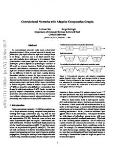
Figure 1: Left: object detections. Right: feature extractor SACT ponder cost (computation time) map for a COCO validation image. The proposed method learns to allocate more computation for the object-like regions of the image.
problems (generating box proposals in object detection) and per-pixel prediction problems (image segmentation, image generation). Additionally, choosing the glimpse positions requires designing a separate prediction network or a heuristic procedure [1]. On the other hand, soft spatial attention models [43, 37] do not allow to save computation since they require evaluating the model at all spatial positions to choose per-position attention weights. We build upon Adaptive Computation Time (ACT) [12] mechanism which was recently proposed for Recurrent Neural Networks (RNNs). We show that ACT can be applied to dynamically choose the number of evaluated layers in Residual Network [16, 17] (the similarity between Residual Networks and RNNs was explored in [30, 13]). Next, we propose Spatially Adaptive Computation Time (SACT) which adapts the amount of computation between spatial positions. While we use SACT mechanism for Residual Networks, it can potentially be used for convolutional LSTM [42] models for video processing [29]. SACT is an end-to-end trainable architecture that incorporates attention into Residual Networks. It learns a deterministic policy that stops computation in a spatial position as soon as the features become “good enough”. Since SACT maintains the alignment between the image and the feature maps, it is well-suited for a wide range of computer vision problems, including multi-output and per-pixel prediction problems.
1. Introduction Deep convolutional networks gained a wide adoption in the image classification problem [24, 39, 40] due to their exceptional accuracy. In recent years deep convolutional networks have become an integral part of state-of-the-art systems for a diverse set of computer vision problems such as object detection [35], image segmentation [33], imageto-text [23, 43], visual question answering [11] and image generation [9]. They have also been shown to be surprisingly effective in non-vision domains, e.g. natural language processing [45] and analyzing the board in the game of Go [38]. A major drawback of deep convolutional networks is their huge computational cost. A natural way to tackle this issue is by using attention to guide the computation, which is similar to how biological vision systems operate [36]. Glimpse-based attention models [27, 34, 2, 21] assume that the problem at hand can be solved by carefully processing a small number of typically rectangular sub-regions of the image. This makes such models unsuitable for multi-output ∗ This
work was done while M. Figurnov was an intern at Google.
1
image conv+pool
residual units
halting scores
pool + fc
0.1 H1 F1
224x224x3
56x56x256 28x28x512
block 1
block 2
14x14x1024
7x7x2048
block 3
block 4
0.1 H2
x1
F2
0.2 H3
x2
F3
0.9 0.1 x1 + 0.1 x2 + 0.2 x3 + 0.6 x4
H4
x3
F4
x4
F5
x5
output
input block of residual units
Figure 2: Residual Network (ResNet) with 101 convolutional layers. Each residual unit contains three convolutional layers. We apply Adaptive Computation Time to each block of ResNet to learn an image-dependent policy of stopping the computation.
Figure 3: Adaptive Computation Time (ACT) for one block of residual units. The computation halts as soon as the cumulative sum of the halting score reaches 1. The remainder is R = 1 − h1 − h2 − h3 = 0.6, the number of evaluated units N = 4, and the ponder cost is ρ = N + R = 4.6. See alg. 1. ACT provides a deterministic and end-to-end learnable policy of choosing the amount of computation.
We evaluate the proposed models on the ImageNet classification problem [8] and find that the SACT outperforms both ACT and non-adaptive baselines. Then, we use SACT as a feature extractor in the Faster R-CNN object detection pipeline [35] and demonstrate results on the challenging COCO dataset [32]. Example detections and ponder cost (computation time) map are presented in fig. 1. SACT achieves significantly superior FLOPs-quality trade-off to the non-adaptive ResNet model. Finally, we demonstrate that the obtained computation time maps are well-correlated with human eye fixations positions, suggesting that a reasonable attention model arises in the model automatically without any explicit supervision.
that restores the number of channels. We use pre-activation ResNet [17] in which each convolutional layer is preceded by batch normalization [20] and ReLU non-linearity. The first units in blocks 2-4 have a stride of 2 and increases the number of output channels by a factor of 2. All other units have equal input and output dimensions. This design choice follows Very Deep Networks [39] and ensures that all units in the network have an equal computational cost (except for the first units of blocks 2-4 having a slightly higher cost). Finally, the obtained feature map is passed through a global average pooling layer [31] and a fully-connected layer that outputs the logits of class probabilities. The global average pooling ensures that the network is fully convolutional meaning that it can be applied to images of varying resolutions without changing the network’s parameters.
2. Method We begin by outlining the recently proposed deep convolutional model Residual Network (ResNet) [16, 17]. Then, we present Adaptive Computation Time, a model which adaptively chooses the number of residual units in ResNet. Finally, we show how this idea can be applied at the spatial position level to obtain Spatially Adaptive Computation Time model.
2.2. Adaptive Computation Time Let us first informally explain Adaptive Computation Time (ACT) before describing it in more detail and providing an algorithm. We add a branch to the outputs of each residual unit which predicts a halting score, a scalar value in the range [0, 1]. The residual units and the halting scores are evaluated sequentially, as shown in fig. 3. As soon as the cumulative sum of the halting score reaches one, all following residual units in this block will be skipped. We set the halting distribution to be the evaluated halting scores with the last value replaced by a remainder. This ensures that the distribution over the values of the halting scores sums to one. The output of the block is then re-defined as a weighted sum of the outputs of residual units, where the weight of each unit is given by the corresponding probability value. Finally, a ponder cost is introduced that is the number of evaluated residual units plus the remainder value. Minimizing the ponder cost increases the halting scores of the non-last residual units making it more likely that the computation would stop earlier. The ponder cost is then multiplied by a constant τ
2.1. Residual Network We first describe the ResNet-101 ImageNet classification architecture (fig. 2). It has been extended for object detection [16, 7] and image segmentation [6] problems. The models we propose are general and can be applied to any ResNet architecture. The first two layers of ResNet-101 are a convolution and a max-pooling layer which together have a total stride of four. Then, a sequence of four blocks is stacked together, each block consisting of multiple stacked residual units. ResNet-101 contains four blocks with 3, 4, 23 and 3 units, respectively. A residual unit has a form F (x) = x + f (x), where the first term is called a shortcut connection and the second term is a residual function. A residual function consists of three convolutional layers: 1 × 1 layer that reduces the number of channels, 3×3 layer that has equal number of input and output channels and 1 × 1 layer 2
Algorithm 1 Adaptive Computation Time for one block of residual units. ACT does not require storing the intermediate residual units outputs. Input: 3D tensor input Input: number of residual units in the block L Input: 0 < ε < 1 Output: 3D tensor output Output: ponder cost ρ 1: x = input 2: c = 0 . Cumulative halting score 3: R = 1 . Remainder value 4: output = 0 . Output of the block 5: ρ = 0 6: for l = 1 . . . L do 7: x = F l (x) 8: if l < L then h = H l (x) 9: else h = 1 10: c += h 11: ρ += 1 12: if c < 1 − ε then 13: output += h · x 14: R −= h 15: else 16: output += R · x 17: ρ += R 18: break 19: return output, ρ
and added to the original loss function. ACT is applied to each block of ResNet independently with the ponder costs summed. Formally, we consider a block of L residual units (boldface denotes tensors of shape Height × Width × Channels): x0 = input,
(1)
xl = F l (xl−1 ) = xl−1 + f l (xl−1 ), l = 1 . . . L,
(2)
L
output = x .
(3)
We introduce a halting score hl ∈ [0, 1] for each residual unit. We define hL = 1 to enforce stopping after the last unit. hl = H l (xl ), l = 1 . . . (L − 1), L
h = 1.
(4) (5)
We choose the halting score function to be a simple linear model on top of the pooled features: hl = H l (xl ) = σ(W l pool(xl ) + bl ),
(6)
where pool is a global average pooling and σ(t) = 1 1+exp(−t) . Next, we determine N , the number of residual units to evaluate, as the index of the first unit where the cumulative halting score exceeds 1 − ε: n n o X N = min n ∈ {1 . . . L} : hl ≥ 1 − ε ,
each other [19, 13], the weighted average also produces a feature representation of the same type. The values of xN +1 , . . . , xL have zero weight and therefore their evaluation can be skipped:
(7)
l=1
where ε is a small constant (e.g., 0.01) that ensures that N can be equal to 1 (the computation stops after the first unit) even though h1 is an output of a sigmoid function meaning that h1 < 1. Additionally, we define the remainder R: R=1−
N −1 X
hl .
output =
L X
pl xl =
N X
l=1
pl xl .
(10)
l=1
Ideally, we would like to directly minimize the number of evaluated units N . However, N is a piecewise constant function of the halting scores that cannot be optimized with gradient descent. Instead, we introduce the ponder cost ρ, an almost everywhere differentiable upper bound on the number of evaluated units N (recall that R ≥ 0):
(8)
l=1
Due to the definition of N in eqn. (7), we have 0 ≤ R ≤ 1. We next transform the halting scores into a halting distribution, which is a discrete distribution over the residual units. Its property is that all the units starting from (N + 1)-st have zero probability: l h if l < N, l p = R if l = N, (9) 0 if l > N.
ρ = N + R.
(11)
When differentiating ρ, we ignore the gradient of N . Also, note that R is not a continuous function of the halting scores [26]. The discontinuities happen in the configurations of halting scores where N changes value. Following [12], we ignore these discontinuities and find that they do not impede training. Algorithm 1 shows the description of ACT. The partial derivative of the ponder cost w.r.t. a halting score hl is ( −1 if l < N, ∂ρ = (12) ∂hl 0 if l ≥ N.
The output of the block is now defined as the outputs of residual units weighted by the halting distribution. Since representations of residual units are compatible with 3
Therefore, minimizing the ponder cost increases h1 , . . . , hN −1 , making the computation stop earlier. This effect is balanced by the original loss function L which also depends on the halting scores via the block output, eqn. (10). Intuitively, the more residual units are used, the better the output, so minimizing L usually increases the weight R of the last used unit’s output xN , which in turn decreases h1 , . . . , hN −1 . ACT has several important advantages. First, it adds very few parameters and computation to the base model. Second, it allows to calculate the output of the block “on the fly” without storing all the intermediate residual unit outputs and halting scores in memory. For example, this would not be possible if the halting distribution were a softmax of halting scores, as done in soft attention [43]. Third, we can recover a block with any constant number of units l ≤ L by setting h1 = · · · = hl−1 = 0, hl = 1. Therefore, ACT is a strict generalization of standard ResNet. We apply ACT to each block independently and then stack the obtained blocks as in the original ResNet. The input of the next block becomes the weighted average of the residual units from the previous block, eqn. (10). A similar connectivity pattern has been explored in [18]. We add the sum of the ponder costs ρk , k = 1 . . . K from the K blocks to the original loss function L: 0
L =L+τ
K X
ρk .
halting scores
1.0
1.0
0.2
0.4
active 0.1
H1
H2
F1
F2
x1
input
inactive
0.7
F3 0.6
x3
x2
output 0.4
block of residual units
Figure 4: Spatially Adaptive Computation Time (SACT) for one block of residual units. We apply ACT to each spatial position of the block. As soon as position’s cumulative halting score reaches 1, we mark it an inactive. See alg. 2. SACT learns to choose the appropriate amount of computation for each spatial position in the block. copy
copy active inactive
residual unit
receptive field
residual unit
Figure 5: Residual unit with active and inactive positions in SACT. This transformation can be implemented efficiently using the perforated convolutional layer [10]. 3x3 conv
(13)
⊕
k=1
The resulting loss function L0 is differentiable and can be optimized using conventional backpropagation. τ ≥ 0 is a regularization coefficient which controls the trade-off between optimizing the original loss function and the ponder cost.
xl
global avg-pooling
ᶥ
fully-connected
hl
Figure 6: SACT halting scores. Halting scores are evaluated fully convolutionally making SACT applicable to images of arbitrary resolution. SACT becomes ACT if the 3 × 3 conv weights are set to zero.
2.3. Spatially Adaptive Computation Time In this section, we present Spatially Adaptive Computation Time (SACT). We adjust the per-position amount of computation by applying ACT to each spatial position of the block, as shown in fig. 4. As we show in the experiments, SACT can learn to focus the computation on the regions of interest. We define the active positions as the spatial locations where the cumulative halting score is less than one. Because an active position might have inactive neighbors, the values for the the inactive positions need to be imputed to evaluate the residual unit in the active positions. We simply copy the previous value for the inactive spatial positions, which is equivalent to setting the residual function f (x) value to zero, as displayed in fig. 5. The evaluation of a block can be stopped completely as soon as all the positions become inactive. Also, the ponder cost is averaged across the spatial positions to make it comparable with the ACT ponder cost. The full algorithm is described in alg. 2.
We define the halting scores for SACT as f l ∗ x + W l pool(x) + bl ), H l (x) = σ(W
(14)
where ∗ denotes a 3 × 3 convolution with a single output channel and pool is a global average-pooling (see fig. 6). SACT is fully convolutional and can be applied to images of any size. Note that SACT is a more general model than ACT, and, f l = 0, consequently, than standard ResNet. If we choose W then the halting scores for all spatial positions coincide. In this case the computation for all the positions halts simultaneously and we recover the ACT model. SACT requires evaluation of the residual function f (x) in just the active spatial positions. This can be performed efficiently using the perforated convolutional layer proposed in [10] (with skipped values replaced by zeros instead of the nearest neighbor’s values). Recall that the residual function 4
Algorithm 2 Spatially Adaptive Computation Time for one block of residual units Input: 3D tensor input Input: number of residual units in the block L Input: 0 < ε < 1 . input and output have different shapes Output: 3D tensor output of shape H × W × C Output: ponder cost ρ ˆ = input 1: x 2: X = {1 . . . H} × {1 . . . W } 3: for all (i, j) ∈ X do 4: aij = true . Active flag 5: cij = 0 . Cumulative halting score 6: Rij = 1 . Remainder value 7: outputij = 0 . Output of the block 8: ρij = 0 . Per-position ponder cost 9: for l = 1 . . . L do 10: if not aij ∀(i, j) ∈ X then break 11: for all (i, j) ∈ X do 12: if aij then xij = F l (ˆ x)ij ˆ ij 13: else xij = x 14: for all (i, j) ∈ X do 15: if not aij then continue 16: if l < L then hij = H l (x)ij 17: else hij = 1 18: cij += hij 19: ρij += 1 20: if cij < 1 − ε then 21: outputij += hij · xij 22: Rij −= hij 23: else 24: outputij += Rij · xij 25: ρij += Rij 26: aij = false ˆP= x 27: x 28: ρ = (i,j)∈X ρij /(HW ) 29: return output, ρ
when the SACT is applied to high-resolution images.
3. Related work The majority of the work on increasing the computational efficiency of deep convolutional networks focuses on static techniques. These include: decompositions of convolutional kernels [22] and pruning of connections [14]. Many of these techniques made their way into the design of the standard deep architectures. For example, Inception [40] and ResNet [16, 17] use factorized convolutional kernels. Recently, several works have considered the problem of varying the amount of computation in computer vision. Cascaded classifiers [28, 44] are used in object detection to quickly reject “easy” negative proposals. Dynamic Capacity Networks [1] use the same amount of computation for all images and use image classification-specific heuristic. PerforatedCNNs [10] vary the amount of computation spatially but not between images. [3] proposes to tune the amount of computation in a fully-connected network using a REINFORCE-trained policy which makes the optimization problem significantly more challenging. BranchyNet [41] is the most similar approach to ours although only applicable to classification problems. It adds classification branches to the intermediate layers of the network. As soon as the entropy of the intermediate classifications is below some threshold, the network’s evaluation halts. Our preliminary experiments with a similar procedure based on ACT (using ACT to choose the number of blocks to evaluate) show that it is inferior to using less units per block.
4. Experiments We first apply ACT and SACT models to the image classification task for the ImageNet dataset [8]. We show that SACT achieves a better FLOPs-accuracy trade-off than ACT by directing computation to the regions of interest. Additionally, SACT improves the accuracy on high-resolution images compared to the ResNet model. Next, we use the obtained SACT model as a feature extractor in the Faster R-CNN object detection pipeline [35] on the COCO dataset [32]. Again we show that we obtain significantly improved FLOPs-mAP trade-off compared to basic ResNet models. Finally, we demonstrate that SACT ponder cost maps correlate well with the position of human eye fixations by evaluating them as a visual saliency model on the cat2000 dataset [4] without any training on this dataset.
consists of a stack of 1 × 1, 3 × 3 and 1 × 1 convolutional layers. The first convolutional layer has to be evaluated in the positions obtained by dilating the active positions set with a 3 × 3 kernel. The second and third layers need to be evaluated just in the active positions. An alternative approach to using the perforated convolutional layer is to tile the halting scores map. Suppose that we share the values of the halting scores hl within k × k tiles. For example, we can perform pooling of hl with a kernel size k ×k and stride k and then upscale the results by a factor of k. Then, all positions in a tile have the same active flag, and we can apply the residual unit densely to just the active tiles, reusing the commonly available convolution routines. k should be sufficiently high to mitigate the overhead of the additional kernel calls and the overlapping computations of the first 1 × 1 convolution. Therefore, tiling is is advisable
4.1. Image classification (ImageNet dataset) First, we train the basic ResNet-50 and ResNet-101 models from scratch using asynchronous SGD with momentum (see the supplementary for the hyperparameters). Our models achieve similar performance to the reference imple5
76.5
79.0
76.0
78.5
75.5 75.0 74.5
SACT SACT baseline ACT ACT baseline ResNet-{50,101}
74.0 73.5 73.0 0.6
0.8
1.0
1.2
Floating point operations
1.4
Validation accuracy (%)
Validation accuracy (%)
mentation1 . For a single center 224 × 224 resolution crop, the reference ResNet-101 model achieves 76.4% accuracy, 92.9% recall@5, while our implementation achieves 76% and 93.1%, respectively. Note that our model is the newer pre-activation ResNet [17] and the reference implementation is the post-activation ResNet [16]. We use ResNet-101 as the basic architecture for ACT and SACT models. Thanks to the end-to-end differentiability and deterministic behaviour, we find the same optimization hyperparameters are applicable for training of ACT and SACT as for the ResNet models. However, special care needs to be taken to address the dead residual unit problem in ACT and SACT models. Since ACT and SACT are deterministic, the last units in the blocks do not get enough training signal and their parameters become obsolete. As a result, the ponder cost saved by not using these units overwhelms the possible initial gains in the original loss function and the units are never used. We observe that while the dead residual units can be recovered during training, this process is very slow. Note that ACT-RNN [12] is not affected by this problem since the parameters for all timesteps are shared. We find two techniques helpful for alleviating the dead residual unit problem. First, we initialize the bias of the halting scores units to a negative value to force the model to use the last units during the initial stages of learning. We use bl = −3 in the experiments which corresponds to initially using 1/σ(bl ) ≈ 21 units. Second, we use a two-stage training procedure by initializing the ACT/SACT network’s weights from the pretrained ResNet-101 model. The halting score weights are still initialized randomly. This greatly simplifies learning of a reasonable halting policy in the beginning of training. As a baseline for ACT and SACT, we consider a nonadaptive ResNet model with a similar number of floating point operations. We take the average numbers of units used in each block in the ACT or SACT model (for SACT we also average over the spatial dimensions) and round them to the nearest integers. Then, we train a ResNet model with such number of units per block. We follow the two-stage training procedure by initializing the network’s parameters with the the first residual units of the full ResNet-101 in each block. This slightly improves the performance compared to using the random initialization. We compare ACT and SACT to ResNet-50, ResNet101 and the baselines in fig. 7. We measure the average per-image number of floating point operations (FLOPs) required for evaluation of the validation set. We treat multiply-add as two floating point operations. The FLOPs are calculated just for the convolution operations (perforated convolution for SACT) since all other operations (nonlinearities, pooling and output averaging in ACT/SACT) have minimal impact on this metric. The ACT models use
1.6 1e10
(a) Test resolution 224 × 224
77.0
SACT SACT baseline ACT ACT baseline ResNet-{50,101}
76.5 76.0 75.5 1.5
2.0
2.5
3.0
Floating point operations
3.5
4.0 1e10
79 78
Validation accuracy (%)
78
Validation accuracy (%)
77.5
(b) Test resolution 352 × 352
79 77 76 75 SACT τ = 0. 001 SACT τ = 0. 001 baseline ACT τ = 0. 0005 ACT τ = 0. 0005 basline ResNet-101
74 73 72 71
78.0
224
288
352
416
77 76 75 SACT τ = 0. 001 SACT τ = 0. 001 baseline ACT τ = 0. 0005 ACT τ = 0. 0005 basline ResNet-101
74 73 72 71 0.0
480
544
Resolution
608
(c) Resolution vs. accuracy
0.2
0.4
0.6
0.8
1.0
Floating point operations
1.2
1.4 1e11
(d) FLOPs vs. accuracy for varying resolution
Figure 7: ImageNet validation set. Comparison of ResNet, ACT, SACT and the respective baselines. All models are trained with 224 × 224 resolution images. SACT outperforms ACT and baselines when applied to images whose resolutions are higher than the training images. The advantage margin grows as resolution difference increases. 3.30 3.15 3.00 2.85 2.70 2.55 2.40 2.25
4.48 4.40 4.32 4.24 4.16 4.08 4.00 3.92
18.0 16.5 15.0 13.5 12.0 10.5 9.0 7.5
3.75 3.50 3.25 3.00 2.75 2.50 2.25 2.00
Figure 8: Ponder cost maps for each block (SACT τ = 0.005, ImageNet validation image). Note that the first block reacts to the low-level features while the last two blocks attempt to localize the object.
τ ∈ {0.0005, 0.001, 0.005, 0.01} and SACT models use τ ∈ {0.001, 0.005, 0.01}. If we increase the image resolution at the test time, as suggested in [17], we observe than SACT outperforms ACT and the baselines. Surprisingly, in this setting SACT has higher accuracy than ResNet-101 model while being computationally cheaper. Such accuracy improvement does not happen for the baseline models or ACT models. We attribute this to the improved scale tolerance provided by the SACT mechanism. The extended results of fig. 7(a,b), including the average number of residual units per block, are presented in the supplementary. We visualize the ponder cost for each block of SACT as heat maps (which we call ponder cost maps henceforth) in fig. 8. More examples of the total SACT ponder cost maps are shown in fig. 9.
4.2. Object detection (COCO dataset) Motivated by the success of SACT in classification of high-resolution images and ignoring uninformative back-
1 https://github.com/KaimingHe/deep-residual-networks
6
28 26 24 22 20 18 16 14 28 26 24 22 20 18 16 14 28 26 24 22 20 18 16 14
Figure 9: ImageNet validation set. SACT (τ = 0.005) ponder cost maps. Top: low ponder cost (19.8-20.55), middle: average ponder cost (23.4-23.6), bottom: high ponder cost (24.9-26.0). SACT typically focuses the computation on the region of interest.
ground, we now turn to a harder problem of object detection. Object detection is typically performed for high-resolution images (such as 1000 × 600, compared to 224 × 224 for ImageNet classification) to allow detection of small objects. Computational redundancy becomes a big issue in this setting since a large image area is often occupied by the background. We use the Faster R-CNN object detection pipeline [35] which consists of three stages. First, the image is processed with a feature extractor. This is the most computationally expensive part. Second, a Region Proposal Network predicts a number of class-agnostic rectangular proposals (typically 300). Third, each proposal box’s features are cropped from the feature map and passed through a box classifier which predicts whether the proposal corresponds to an object, the class of this object and refines the boundaries. We train the model end-to-end using asynchronous SGD with momentum, employing Tensorflow’s crop_and_resize operation, which is similar to the Spatial Transformer Network [21], to perform cropping of the region proposals. The training hyperparameters are provided in the supplementary. We use ResNet blocks 1-3 as a feature extractor and block 4 as a box classifier, as suggested in [16]. We reuse the models pretrained on the ImageNet classification task and fine-tune them for COCO detection. For SACT, the ponder cost penalty τ is only applied to the feature extractor (we use the same value as for ImageNet classification). We use COCO train for training and COCO val for evaluation (instead of the combined train+val set which is sometimes used in the literature). We do not employ multiscale inference, iterative box refinement or global context. We find that SACT achieves superior speed-mAP tradeoff compared to the baseline of using non-adaptive ResNet as a feature extractor (see table 1). SACT τ = 0.005 model
Feature extractor FLOPs (%) mAP @ [.5, .95] (%) ResNet-101 [16] 100 27.2 ResNet-50 (our impl.) 46.6 25.56 SACT τ = 0.005 56.0 27.61 SACT τ = 0.001 72.4 29.04 ResNet-101 (our impl.) 100 29.24
Table 1: COCO val set. Faster R-CNN with SACT results. FLOPs are average feature extractor floating point operations relative to ResNet-101 (that does 1.42E+11 operations). SACT improves the FLOPs-mAP trade-off compared to using ResNet without adaptive computation.
has slightly higher FLOPs count than ResNet-50 and 2.1 points better mAP. Note that this SACT model outperforms the originally reported result for ResNet-101, 27.2 mAP [16]. Several examples are presented in fig. 10.
4.3. Visual saliency (cat2000 dataset) We now show that SACT ponder cost maps correlate well with human attention. To do that, we use a large dataset of visual saliency: the cat2000 dataset [4]. The dataset is obtained by showing 4,000 images of 20 scene categories to 24 human subjects and recording their eye fixation positions. The ground-truth saliency map is a heat map of the eye fixation positions. We do not train the SACT models on this dataset and simply reuse the ImageNet- and COCO-trained models. Cat2000 saliency maps exhibit a strong center bias. Most images contain a blob of saliency in the center even when there is no object of interest located there. Since our model is fully convolutional, we cannot learn such bias even if we trained on the saliency data. Therefore, we combine our ponder cost maps with a constant center-biased map. 7
24 22 20 18 16 14 12 10 8
24 22 20 18 16 14 12 10 8
Figure 10: COCO testdev set. Detections and feature extractor ponder cost maps (τ = 0.005). SACT allocates much more computation to the object-like regions of the image.
Model AUC-Judd (%) Center baseline [4] 83.4 DeepFix [25] 87† “Infinite humans” [4] 90† ImageNet SACT τ = 0.005 84.6 COCO SACT τ = 0.005 84.7
Table 2: cat2000 validation set. † - results for the test set. SACT ponder cost maps work as a visual saliency model even without explicit supervision.
We resize the 1920 × 1080 cat2000 images to 320 × 180 for ImageNet model and to 640 × 360 for COCO model and pass them through the SACT model. Following [4], we consider a linear combination of the Gaussian blurred ponder cost map normalized to [0, 1] range and a “center baseline,” a Gaussian centered at the middle of the image. Full description of the combination scheme is provided in the supplementary. The first half of the training set images for every scene category is used for determining the optimal values of the Gaussian blur kernel size and the center baseline multiplier, while the second half is used for validation. Table 2 presents the AUC-Judd [5] metric, the area under the ROC-curve for the saliency map as a predictor for eye fixation positions. SACT outperforms the na¨ıve center baseline. Compared to the state-of-the-art deep model DeepFix [25] method, SACT does competitively. Examples are shown in fig. 11.
Figure 11: cat2000 saliency dataset. Left to right: image, human saliency, SACT ponder cost map (COCO model, τ = 0.005) with postprocessing (see text) and softmax with temperature 1/5. Note the center bias of the dataset. SACT model performs surprisingly well on out-of-domain images such as art and fractals.
trainable, deterministic and can be viewed as a black-box feature extractor. We show its effectiveness in image classification and object detection problems. The amount of per-position computation in this model correlates well with the human eye fixation positions, suggesting that this model captures the important parts of the image. We hope that this paper will lead to a wider adoption of attention and adaptive computation time in large-scale computer vision systems. Acknowledgments. Dmitry Vetrov is supported by RFBR project No. 15-31-20596 (mol-a-ved) and Microsoft: Moscow State University Joint Research Center (RPD 1053945). Ruslan Salakhutdinov is supported in part by
5. Conclusion We present a Residual Network based model with a spatially varying computation time. This model is end-to-end 8
ONR grants N00014-13-1-0721, N00014-14-1-0232, and the ADeLAIDE grant FA8750-16C-0130-001.
[19] G. Huang, Y. Sun, Z. Liu, D. Sedra, and K. Weinberger. Deep networks with stochastic depth. ECCV, 2016. 3 [20] S. Ioffe and C. Szegedy. Batch normalization: Accelerating deep network training by reducing internal covariate shift. arXiv preprint arXiv:1502.03167, 2015. 2 [21] M. Jaderberg, K. Simonyan, A. Zisserman, and K. Kavukcuoglu. Spatial transformer networks. NIPS, 2015. 1, 7 [22] M. Jaderberg, A. Vedaldi, and A. Zisserman. Speeding up convolutional neural networks with low rank expansions. BMVC, 2014. 5 [23] A. Karpathy and L. Fei-Fei. Deep visual-semantic alignments for generating image descriptions. CVPR, 2015. 1 [24] A. Krizhevsky, I. Sutskever, and G. E. Hinton. Imagenet classification with deep convolutional neural networks. NIPS, 2012. 1 [25] S. S. Kruthiventi, K. Ayush, and R. V. Babu. Deepfix: A fully convolutional neural network for predicting human eye fixations. arXiv preprint arXiv:1510.02927, 2015. 8 [26] H. Larochelle. My notes on adaptive computation time for recurrent neural networks. Blog post https://goo.gl/QxBucH, 2016. 3 [27] H. Larochelle and G. E. Hinton. Learning to combine foveal glimpses with a third-order boltzmann machine. NIPS, 2010. 1 [28] H. Li, Z. Lin, X. Shen, J. Brandt, and G. Hua. A convolutional neural network cascade for face detection. CVPR, 2015. 5 [29] Z. Li, E. Gavves, M. Jain, and C. G. Snoek. Videolstm convolves, attends and flows for action recognition. arXiv preprint arXiv:1607.01794, 2016. 1 [30] Q. Liao and T. Poggio. Bridging the gaps between residual learning, recurrent neural networks and visual cortex. arXiv preprint arXiv:1604.03640, 2016. 1 [31] M. Lin, Q. Chen, and S. Yan. Network in network. ICLR, 2014. 2 [32] T.-Y. Lin, M. Maire, S. Belongie, J. Hays, P. Perona, D. Ramanan, P. Doll´ar, and C. L. Zitnick. Microsoft coco: Common objects in context. ECCV, 2014. 2, 5 [33] J. Long, E. Shelhamer, and T. Darrell. Fully convolutional networks for semantic segmentation. CVPR, 2015. 1 [34] V. Mnih, N. Heess, A. Graves, et al. Recurrent models of visual attention. NIPS, 2014. 1 [35] S. Ren, K. He, R. Girshick, and J. Sun. Faster r-cnn: Towards real-time object detection with region proposal networks. NIPS, 2015. 1, 2, 5, 7, 11 [36] R. A. Rensink. The dynamic representation of scenes. Visual cognition, 7(1-3), 2000. 1 [37] S. Sharma, R. Kiros, and R. Salakhutdinov. Action recognition using visual attention. ICLR Workshop, 2016. 1 [38] D. Silver, A. Huang, C. J. Maddison, A. Guez, L. Sifre, G. Van Den Driessche, J. Schrittwieser, I. Antonoglou, V. Panneershelvam, M. Lanctot, et al. Mastering the game of go with deep neural networks and tree search. Nature, 529(7587), 2016. 1 [39] K. Simonyan and A. Zisserman. Very deep convolutional networks for large-scale image recognition. ICLR, 2015. 1, 2
References [1] A. Almahairi, N. Ballas, T. Cooijmans, Y. Zheng, H. Larochelle, and A. Courville. Dynamic capacity networks. ICML, 2016. 1, 5 [2] J. Ba, V. Mnih, and K. Kavukcuoglu. Multiple object recognition with visual attention. ICLR, 2015. 1 [3] E. Bengio, P.-L. Bacon, J. Pineau, and D. Precup. Conditional computation in neural networks for faster models. ICLR Workshop, 2016. 5 [4] Z. Bylinskii, T. Judd, A. Borji, L. Itti, F. Durand, A. Oliva, and A. Torralba. Mit saliency benchmark. http://saliency.mit.edu/. 5, 7, 8 [5] Z. Bylinskii, T. Judd, A. Oliva, A. Torralba, and F. Durand. What do different evaluation metrics tell us about saliency models? arXiv preprint arXiv:1604.03605, 2016. 8 [6] L.-C. Chen, G. Papandreou, I. Kokkinos, K. Murphy, and A. L. Yuille. Deeplab: Semantic image segmentation with deep convolutional nets, atrous convolution, and fully connected crfs. arXiv preprint arXiv:1606.00915, 2016. 2 [7] J. Dai, Y. Li, K. He, and J. Sun. R-fcn: Object detection via region-based fully convolutional networks. NIPS, 2016. 2 [8] J. Deng, W. Dong, R. Socher, L.-J. Li, K. Li, and L. Fei-Fei. Imagenet: A large-scale hierarchical image database. CVPR, 2009. 2, 5 [9] A. Dosovitskiy, J. Tobias Springenberg, and T. Brox. Learning to generate chairs with convolutional neural networks. CVPR, 2015. 1 [10] M. Figurnov, A. Ibraimova, D. Vetrov, and P. Kohli. PerforatedCNNs: Acceleration through elimination of redundant convolutions. NIPS, 2016. 4, 5 [11] A. Fukui, D. H. Park, D. Yang, A. Rohrbach, T. Darrell, and M. Rohrbach. Multimodal compact bilinear pooling for visual question answering and visual grounding. arXiv preprint arXiv:1606.01847, 2016. 1 [12] A. Graves. Adaptive computation time for recurrent neural networks. arXiv preprint arXiv:1603.08983, 2016. 1, 3, 6 [13] K. Greff, R. Srivastava, and J. Schmidhuber. Highway and residual networks learn unrolled iterative estimation. ICLR 2017 submission. 1, 3 [14] S. Han, H. Mao, and W. J. Dally. Deep compression: Compressing deep neural network with pruning, trained quantization and huffman coding. ICLR, 2016. 5 [15] K. He, X. Zhang, S. Ren, and J. Sun. Delving deep into rectifiers: Surpassing human-level performance on imagenet classification. CVPR, 2015. 11 [16] K. He, X. Zhang, S. Ren, and J. Sun. Deep residual learning for image recognition. CVPR, 2016. 1, 2, 5, 6, 7 [17] K. He, X. Zhang, S. Ren, and J. Sun. Identity mappings in deep residual networks. ECCV, 2016. 1, 2, 5, 6 [18] G. Huang, Z. Liu, and K. Q. Weinberger. Densely connected convolutional networks. arXiv preprint arXiv:1608.06993, 2016. 4
9
[40] C. Szegedy, W. Liu, Y. Jia, P. Sermanet, S. Reed, D. Anguelov, D. Erhan, V. Vanhoucke, and A. Rabinovich. Going deeper with convolutions. CVPR, 2015. 1, 5 [41] S. Teerapittayanon, B. McDanel, and H. Kung. Branchynet: Fast inference via early exiting from deep neural networks. ICPR, 2016. 5 [42] S. Xingjian, Z. Chen, H. Wang, D.-Y. Yeung, W.-k. Wong, and W.-c. Woo. Convolutional lstm network: A machine learning approach for precipitation nowcasting. In NIPS, 2015. 1 [43] K. Xu, J. Ba, R. Kiros, K. Cho, A. Courville, R. Salakhutdinov, R. S. Zemel, and Y. Bengio. Show, attend and tell: Neural image caption generation with visual attention. ICML, 2015. 1, 4 [44] F. Yang, W. Choi, and Y. Lin. Exploit all the layers: Fast and accurate cnn object detector with scale dependent pooling and cascaded rejection classifiers. CVPR, 2016. 5 [45] X. Zhang, J. Zhao, and Y. LeCun. Character-level convolutional networks for text classification. NIPS, 2015. 1
10
Supplementary materials In the supplementary materials we present the implementation details for the experiments described in the paper. Additionally, we present the extended results of ACT, SACT and ResNet on ImageNet validation set, including the number of residual units per block, in table 3.
A. Implementation details A.1. Image classification (ImageNet) Optimization hyperparameters. ResNet, ACT and SACT use the same hyperparameters. We train the networks with 50 workers running asynchronous SGD with momentum 0.9, weight decay 0.0001 and batch size 32. The training is halted upon convergence after 150 − 160 epochs. Learning rate is initially set to 0.05 and lowered by a factor of 10 after every 30 epochs. Batch normalization parameters are: epsilon 1e-5, moving average decay 0.997. The parameters of the network are initialized with a variance scaling initializer [15]. Data augmentation. We use the Inception v3 data augmentation procedure2 which includes horizontal flipping, scale, aspect ratio, color augmentation. For the ImageNet images with a provided bounding box, we perform cropping based on the distorted bounding box. For evaluation, we take a single central crop of 87.5% of the original image’s area and then resize this crop to the target resolution.
A.2. Object detection (COCO) ResNet and SACT models use the same hyperparameters. The images are upscaled (preserving aspect ratio) so that the smaller side is at least 600 pixels. For data augmentation, we use random horizontal flipping as is described in [35]. We do not employ atrous convolution algorithm. Optimization hyperparameters. We use distributed training with 9 workers running asynchronous SGD with momentum 0.9 and a batch size of 1. The learning rate is initially set to 0.0003 and lowered by a factor of 10 after the 800 thousandth and 1 millionth training iterations (batches). The training proceeds for a total of 1.2 million iterations. Batch normalization parameters are fixed to the values obtained on ImageNet during training. Faster R-CNN hyperparameters. Other than the training method, our hyperparameters for the Faster R-CNN model closely follow those recommended by the original paper [35]. The anchors are generated in the same way, sampled from a regular grid of stride 16. One change relative to the original paper is the addition of an additional anchor size, so full set of anchor box sizes are {64, 128, 256, 512}, with the height and width also varying for each choice of the aspect ratios {0.5, 1, 2}. We use 300 object proposals per image. Non-maximum suppression is performed with 0.6 IoU threshold. For each proposal, the features are cropped into a 28 × 28 box with crop_and_resize TensorFlow operation, then pooled to 7 × 7.
A.3. Visual saliency (cat2000) Here we describe the postprocessing procedure used in the visual saliency experiments. Consider a ponder cost map ρij , i ∈ {1, . . . , H}, j ∈ {1, . . . , W }. Let Gs be a Gaussian filter with a standard deviation s. We first normalize this map to [0, 1]: ρnij =
ρij − ρmin , i ∈ {1, . . . , H}, j ∈ {1, . . . , W }. ρmax − ρmin
(15)
where ρmin = min ρij ij
(16)
and similarily for max. Then, we blur the ponder cost map by convolving the Gaussian filter with ρ: ρnb = Gs ∗ ρn .
(17)
We obtain a baseline map Bij by rescaling the reference centered Gaussian3 to H × W resolution. We use this map with a weight γ > 0. 2 https://github.com/tensorflow/models/blob/master/inception/inception/image_processing.py 3 https://github.com/cvzoya/saliency/blob/master/code_forOptimization/center.mat
11
Network ResNet-50 ResNet-101 ACT τ = 0.01 Baseline ACT τ = 0.005 Baseline ACT τ = 0.001 Baseline ACT τ = 0.0005 Baseline SACT τ = 0.01 Baseline SACT τ = 0.005 Baseline SACT τ = 0.001 Baseline
FLOPs 8.18E+09 1.56E+10 6.38E+09 6.43E+09 8.13E+09 8.18E+09 1.15E+10 1.17E+10 1.34E+10 1.34E+10 6.61E+09 6.43E+09 1.11E+10 1.08E+10 1.44E+10 1.43E+10
Test resolution 224 × 224 Residual units Accuracy 3, 4, 6, 3 74.56% 3, 4, 23, 3 76.01% 2.9, 2.7, 3.3, 3.0 73.17% 3, 3, 3, 3 73.03% 3.0, 4.0, 5.9, 3.0 73.95% 3, 4, 6, 3 74.34% 3.0, 4.0, 13.7, 3.0 75.01% 3, 4, 14, 3 75.69% 3.0, 4.0, 17.9, 3.0 75.26% 3, 4, 18, 3 75.88% 2.6, 2.4, 4.0, 2.7 73.24% 3, 2, 4, 3 73.33% 2.3, 3.8, 13.1, 2.7 75.60% 2, 4, 13, 3 75.57% 3.0, 4.0, 19.6, 2.9 75.84% 3, 4, 20, 3 76.06%
Recall@5 92.37% 93.15% 91.55% 91.68% 92.02% 92.19% 92.63% 93.02% 92.82% 93.02% 91.49% 91.67% 92.83% 92.86% 93.10% 93.17%
FLOPs 2.02E+10 3.85E+10 1.58E+10 1.59E+10 2.01E+10 2.02E+10 2.95E+10 2.88E+10 3.31E+10 3.31E+10 1.65E+10 1.59E+10 2.78E+10 2.67E+10 3.58E+10 3.53E+10
Test resolution 352 × 352 Residual units Accuracy Recall@5 3, 4, 6, 3 76.82% 93.80% 3, 4, 23, 3 78.37% 94.60% 2.9, 2.7, 3.3, 3.0 75.85% 93.18% 3, 3, 3, 3 75.61% 93.14% 3.0, 4.0, 6.0, 3.0 76.56% 93.58% 3, 4, 6, 3 76.62% 93.63% 3.0, 4.0, 14.7, 3.0 77.67% 94.14% 3, 4, 14, 3 77.73% 94.31% 3.0, 4.0, 17.9, 3.0 77.89% 94.13% 3, 4, 18, 3 78.10% 94.43% 2.6, 2.5, 4.1, 2.8 76.31% 93.43% 3, 2, 4, 3 75.99% 93.26% 2.3, 3.9, 13.4, 2.8 78.44% 94.46% 2, 4, 13, 3 77.57% 94.21% 3.0, 4.0, 19.9, 3.0 78.74% 94.69% 3, 4, 20, 3 78.23% 94.38%
Table 3: ImageNet validation set. Comparison of ResNet, ACT, SACT and the respective baselines. All models are trained with 224 × 224 resolution images. For ACT and SACT, the number of residual units in each block N is averaged over the objects and spatial dimensions.
Finally, the postprocessed ponder cost map is defined as a normalized blurred ponder cost map plus the weighted center baseline map: nb ρnbc (18) ij = ρij + γBij , i ∈ {1, . . . , H}, j ∈ {1, . . . , W }. ρnbc depends on two hyperparameters: the Gaussian filter standard deviation s and baseline map weight γ. The values are tuned via grid search. In the experiments in the paper, we use s = 10, γ = 0.005 for both models.
12