Sep 15, 2003 - Contents. Acknowledgements iv. List of Figures ix. Summary ..... performance of our protocol in terms of packet delivery ratio and routing traffic is ...... A tutorial on learning with bayesian networks, 1995. http://citeseer.nj.nec.
SWARM: Cooperative Reinforcement Learning for Routing in Ad-hoc Networks
Eoin Curran
A thesis submitted to the University of Dublin, Trinity College in partial fulfillment of the requirements for the degree of Master of Science
September 2003
Declaration
I, the undersigned, declare that this work has not previously been submitted to this or any other University, and that unless otherwise stated, it is entirely my own work.
Eoin Curran
Dated: 15th September 2003
Permission to Lend and/or Copy
I, the undersigned, agree that Trinity College Library may lend or copy this thesis upon request.
Eoin Curran
Dated: 15th September 2003
Acknowledgements I would like to thank my supervisor Jim Dowling for his great help and patience during the course of my research. I would also like to thank my family for their support and understanding. Lastly, I would like to thank the Networks and Distributed Systems class of 2003 for making the past year so enjoyable and worthwhile.
Eoin Curran University of Dublin, Trinity College September 2003
iv
Contents Acknowledgements
iv
List of Figures
ix
Summary
x
Chapter 1 1.1
1.2
1.3
1.4
Background: Ad-hoc Routing
1
What is Ad-hoc? . . . . . . . . . . . . . . . . . . . . . . . . . . . . . . . . . . . . . . . . . . .
1
1.1.1
MANET . . . . . . . . . . . . . . . . . . . . . . . . . . . . . . . . . . . . . . . . . . .
2
1.1.2
Mesh Networks . . . . . . . . . . . . . . . . . . . . . . . . . . . . . . . . . . . . . . . .
2
1.1.3
Zeroconf . . . . . . . . . . . . . . . . . . . . . . . . . . . . . . . . . . . . . . . . . . .
2
IEEE 802.11 - Wireless Ethernet . . . . . . . . . . . . . . . . . . . . . . . . . . . . . . . . . . .
3
1.2.1
Physical Layer . . . . . . . . . . . . . . . . . . . . . . . . . . . . . . . . . . . . . . . .
3
1.2.2
Media Access Control Layer . . . . . . . . . . . . . . . . . . . . . . . . . . . . . . . . .
3
1.2.3
802.11 in multi-hop networks . . . . . . . . . . . . . . . . . . . . . . . . . . . . . . . .
4
1.2.3.1
Interaction of MAC layer with TCP . . . . . . . . . . . . . . . . . . . . . . . .
4
1.2.3.2
Performance Measurements: Loss Rates . . . . . . . . . . . . . . . . . . . . .
4
1.2.3.3
Theoretical Capacity of Ad-Hoc Networks . . . . . . . . . . . . . . . . . . . .
5
Ad-hoc Routing Protocols . . . . . . . . . . . . . . . . . . . . . . . . . . . . . . . . . . . . . .
5
1.3.1
Pro-active protocols . . . . . . . . . . . . . . . . . . . . . . . . . . . . . . . . . . . . .
6
1.3.2
On-demand protocols . . . . . . . . . . . . . . . . . . . . . . . . . . . . . . . . . . . . .
6
Ad-hoc Connectivity . . . . . . . . . . . . . . . . . . . . . . . . . . . . . . . . . . . . . . . . .
7
1.4.1
Lei/Perkins - DSDV and Mobile IP . . . . . . . . . . . . . . . . . . . . . . . . . . . . .
7
1.4.2
Broch/Maltz/Johnson - DSR . . . . . . . . . . . . . . . . . . . . . . . . . . . . . . . . .
8
1.4.3
MIPMANET . . . . . . . . . . . . . . . . . . . . . . . . . . . . . . . . . . . . . . . . .
9
1.4.4
Perkins/Sun/Belding-Royer . . . . . . . . . . . . . . . . . . . . . . . . . . . . . . . . .
10
1.4.5
MEWLANA . . . . . . . . . . . . . . . . . . . . . . . . . . . . . . . . . . . . . . . . .
10
1.4.6
LUNAR . . . . . . . . . . . . . . . . . . . . . . . . . . . . . . . . . . . . . . . . . . . .
11
1.4.7
Hybrid Proactive and Reactive Mobile IP . . . . . . . . . . . . . . . . . . . . . . . . . .
12
v
1.4.8 1.5
LocustWorld MeshAP . . . . . . . . . . . . . . . . . . . . . . . . . . . . . . . . . . . .
12
Evaluation of Ad-hoc Routing Protocols . . . . . . . . . . . . . . . . . . . . . . . . . . . . . . .
13
1.5.1
Mobility Model . . . . . . . . . . . . . . . . . . . . . . . . . . . . . . . . . . . . . . . .
13
1.5.2
Network Scenario . . . . . . . . . . . . . . . . . . . . . . . . . . . . . . . . . . . . . . .
13
1.5.2.1
MANET networking contexts . . . . . . . . . . . . . . . . . . . . . . . . . . .
13
1.5.2.2
Additional Parameters for Internet Connectivity . . . . . . . . . . . . . . . . .
14
Example Network Scenarios . . . . . . . . . . . . . . . . . . . . . . . . . . . . . . . . .
14
1.5.3.1
Random Scenario . . . . . . . . . . . . . . . . . . . . . . . . . . . . . . . . .
14
1.5.3.2
Scenario-Based Performance Analysis . . . . . . . . . . . . . . . . . . . . . .
15
1.5.3.3
(Sub)Urban Mesh Network . . . . . . . . . . . . . . . . . . . . . . . . . . . .
15
1.5.3.4
WAND . . . . . . . . . . . . . . . . . . . . . . . . . . . . . . . . . . . . . . .
15
Performance Evaluation . . . . . . . . . . . . . . . . . . . . . . . . . . . . . . . . . . .
16
1.5.4.1
Network Simulation . . . . . . . . . . . . . . . . . . . . . . . . . . . . . . . .
16
1.5.4.2
Real-world evaluation . . . . . . . . . . . . . . . . . . . . . . . . . . . . . . .
16
1.5.4.3
Performance criteria . . . . . . . . . . . . . . . . . . . . . . . . . . . . . . . .
17
Miscellaneous . . . . . . . . . . . . . . . . . . . . . . . . . . . . . . . . . . . . . . . .
17
1.5.5.1
Implementation . . . . . . . . . . . . . . . . . . . . . . . . . . . . . . . . . .
17
Other Research . . . . . . . . . . . . . . . . . . . . . . . . . . . . . . . . . . . . . . . . . . . .
17
1.6.1
Artificial Intelligence / Mobile Agents for Routing . . . . . . . . . . . . . . . . . . . . .
17
1.6.1.1
Swarm Intelligence for Routing . . . . . . . . . . . . . . . . . . . . . . . . . .
17
1.6.1.2
Agent-based DVR . . . . . . . . . . . . . . . . . . . . . . . . . . . . . . . . .
19
Message Flooding and Broadcast Storms . . . . . . . . . . . . . . . . . . . . . . . . . .
19
1.6.2.1
The Flooding Problem . . . . . . . . . . . . . . . . . . . . . . . . . . . . . . .
19
1.6.2.2
Broadcast Storms . . . . . . . . . . . . . . . . . . . . . . . . . . . . . . . . .
20
1.6.2.3
Probabilistic Broadcast and Phase transitions . . . . . . . . . . . . . . . . . . .
21
1.6.2.4
Gossip based Ad Hoc Routing . . . . . . . . . . . . . . . . . . . . . . . . . .
21
Service-based Routing . . . . . . . . . . . . . . . . . . . . . . . . . . . . . . . . . . . .
22
1.5.3
1.5.4
1.5.5
1.6
1.6.2
1.6.3 Chapter 2
Reinforcement Learning and Swarm Intelligence
23
2.1
Overview . . . . . . . . . . . . . . . . . . . . . . . . . . . . . . . . . . . . . . . . . . . . . . .
23
2.2
Reinforcement-Learning . . . . . . . . . . . . . . . . . . . . . . . . . . . . . . . . . . . . . . .
24
2.2.1
Definition of Optimal Policy . . . . . . . . . . . . . . . . . . . . . . . . . . . . . . . . .
25
2.2.1.1
Long-term Reward Model . . . . . . . . . . . . . . . . . . . . . . . . . . . . .
25
2.2.1.2
Optimal Value Function and Optimal Policy . . . . . . . . . . . . . . . . . . .
25
Learning Strategies for Reinforcement Learning Problems . . . . . . . . . . . . . . . . . . . . .
26
2.3.1
Model-based versus Model-free . . . . . . . . . . . . . . . . . . . . . . . . . . . . . . .
26
2.3.2
Q-Learning. Model-Based and Model-Free . . . . . . . . . . . . . . . . . . . . . . . . .
27
2.3.3
Prioritized Sweeping . . . . . . . . . . . . . . . . . . . . . . . . . . . . . . . . . . . . .
27
2.3
vi
2.4
2.3.4
Advantage of Model-based Methods . . . . . . . . . . . . . . . . . . . . . . . . . . . . .
28
2.3.5
Exploration versus Exploitation . . . . . . . . . . . . . . . . . . . . . . . . . . . . . . .
28
Swarm Intelligence and Ant-colony Optimisation . . . . . . . . . . . . . . . . . . . . . . . . . .
28
2.4.1
ACO Learning Strategy . . . . . . . . . . . . . . . . . . . . . . . . . . . . . . . . . . . .
29
2.4.2
The Agent Metaphor in ACO and RL . . . . . . . . . . . . . . . . . . . . . . . . . . . .
31
2.4.3
ACO as a learning strategy for RL . . . . . . . . . . . . . . . . . . . . . . . . . . . . . .
31
Chapter 3 3.1
The SWARM Ad-hoc Routing protocol
33
Model of Reinforcements in Wireless Network . . . . . . . . . . . . . . . . . . . . . . . . . . .
33
3.1.1
Model of long-term reward . . . . . . . . . . . . . . . . . . . . . . . . . . . . . . . . . .
34
3.2
Link Delivery Ratios . . . . . . . . . . . . . . . . . . . . . . . . . . . . . . . . . . . . . . . . .
35
3.3
Optimal Exploitative Policy . . . . . . . . . . . . . . . . . . . . . . . . . . . . . . . . . . . . . .
36
3.4
Cost of Transmission, Physical Interpretation . . . . . . . . . . . . . . . . . . . . . . . . . . . .
38
3.5
The SWARM Learning Strategy for Ad-hoc Routing . . . . . . . . . . . . . . . . . . . . . . . .
39
3.6
Exploration in the ad-hoc network . . . . . . . . . . . . . . . . . . . . . . . . . . . . . . . . . .
40
3.6.1
Exploration Action . . . . . . . . . . . . . . . . . . . . . . . . . . . . . . . . . . . . . .
41
3.6.2
Greedy Heuristic . . . . . . . . . . . . . . . . . . . . . . . . . . . . . . . . . . . . . . .
41
Feedback in the ad-hoc network . . . . . . . . . . . . . . . . . . . . . . . . . . . . . . . . . . .
42
3.7.1
Promiscuous Receive . . . . . . . . . . . . . . . . . . . . . . . . . . . . . . . . . . . . .
42
3.7.2
Silent Feedback . . . . . . . . . . . . . . . . . . . . . . . . . . . . . . . . . . . . . . . .
43
3.7.3
Notes . . . . . . . . . . . . . . . . . . . . . . . . . . . . . . . . . . . . . . . . . . . . .
43
3.7.3.1
Bi-directionality . . . . . . . . . . . . . . . . . . . . . . . . . . . . . . . . . .
43
3.7.3.2
Pro-active responses . . . . . . . . . . . . . . . . . . . . . . . . . . . . . . . .
43
Implementation Details . . . . . . . . . . . . . . . . . . . . . . . . . . . . . . . . . . . . . . . .
43
3.8.1
Packet Format . . . . . . . . . . . . . . . . . . . . . . . . . . . . . . . . . . . . . . . .
44
3.8.2
Routing Tables . . . . . . . . . . . . . . . . . . . . . . . . . . . . . . . . . . . . . . . .
44
3.8.3
Routing Protocol Parameters . . . . . . . . . . . . . . . . . . . . . . . . . . . . . . . . .
45
3.8.4
Routing Algorithm . . . . . . . . . . . . . . . . . . . . . . . . . . . . . . . . . . . . . .
47
3.7
3.8
Chapter 4 4.1
Protocol Evaluation
52
WAND Network Scenario . . . . . . . . . . . . . . . . . . . . . . . . . . . . . . . . . . . . . .
52
4.1.1
Relationship between Temperature and Exploration Action . . . . . . . . . . . . . . . . .
54
4.1.2
Number of Actions Considered: Greedy Heuristic . . . . . . . . . . . . . . . . . . . . . .
57
4.1.3
Silent Feedback: route decay, event window . . . . . . . . . . . . . . . . . . . . . . . . .
57
4.1.4
One-way Traffic: Pro-active responses . . . . . . . . . . . . . . . . . . . . . . . . . . . .
59
4.1.5
Conclusion . . . . . . . . . . . . . . . . . . . . . . . . . . . . . . . . . . . . . . . . . .
59
4.2
Comparison to AODV and DSR . . . . . . . . . . . . . . . . . . . . . . . . . . . . . . . . . . .
62
4.3
Conclusions . . . . . . . . . . . . . . . . . . . . . . . . . . . . . . . . . . . . . . . . . . . . . .
64
vii
Conclusion
68
Bibliography
69
viii
List of Figures 2.1
Agent Interaction with the Reinforcement-Learning Model . . . . . . . . . . . . . . . . . . . . .
24
3.1
Reinforcement Learning Model for Ad-hoc Routing . . . . . . . . . . . . . . . . . . . . . . . . .
35
3.2
Counting Events within a window . . . . . . . . . . . . . . . . . . . . . . . . . . . . . . . . . .
37
3.3
Greedy Heuristic: Permitted actions . . . . . . . . . . . . . . . . . . . . . . . . . . . . . . . . .
42
3.4
Routing Tables . . . . . . . . . . . . . . . . . . . . . . . . . . . . . . . . . . . . . . . . . . . .
44
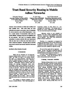
4.1
Simulation Arena, showing fixed node positions (transmission range is 100m) . . . . . . . . . . .
54
4.2
Delivery Ratio versus Temperature, varying exploration utility . . . . . . . . . . . . . . . . . . .
55
4.3
Correlation of performance with −T ue
−T ue
. . . . . . . . . . . . . . . . . . . . . . . . . . . . . . . . .
55
4.4
Effect of Temperature with
’factored out’ . . . . . . . . . . . . . . . . . . . . . . . . . . . .
56
4.5
Ratio of exploration actions . . . . . . . . . . . . . . . . . . . . . . . . . . . . . . . . . . . . . .
57
4.6
Effect of M INIMUM R EWARD heuristic . . . . . . . . . . . . . . . . . . . . . . . . . . . . . . . .
58
4.7
Effect of decay rate / silent feedback . . . . . . . . . . . . . . . . . . . . . . . . . . . . . . . . .
60
4.8
Effect of sending pro-active routing packets . . . . . . . . . . . . . . . . . . . . . . . . . . . . .
61
4.9
Performance with Varying Load. 64 byte packets . . . . . . . . . . . . . . . . . . . . . . . . . .
64
4.10 Performance with Varying Load. 512 byte packets . . . . . . . . . . . . . . . . . . . . . . . . . .
65
4.11 SWARM Delivery Cost performance under load. 512 byte packets. . . . . . . . . . . . . . . . . .
66
4.12 End-to-end latency performance under load. 512 byte packets. . . . . . . . . . . . . . . . . . . .
67
ix
Summary Existing ad-hoc routing protocols are based on a discrete, bimodal model for links between nodes: a link either exists or is broken. This model usually considers only the most recent transmission as determining the state of the link. Unfortunately, this model cannot distinguish transmissions which fail due to interference or congestion from those which fail due to their target being out of transmission range. This thesis presents a new ad-hoc routing protocol based on a continuous (rather than discrete) model for links within the network. We use a statistical measure of link performance over time to represent the quality of the link. We propose that such a model is required for efficient operation within real-world wireless networks. In order to define optimal routes in a network with links of variable quality, we model ad-hoc routing as a cooperative reinforcement-learning problem. Cooperative reinforcement-learning describes a class of problems within machine learning in which agents attempt to optimize it’s interaction with a dynamic environment through trial and error and information sharing. We assign a value to routes that is representative of the costs to the agents using that route. The ad-hoc routing problem is thus expressed as the optimization of the value of routes. Our model of link quality is a statistical one and requires data to be gathered over time. We devise a learning strategy that gathers information about available routes and the quality of their links over time. This learning strategy operates in an on-demand manner, gathering information only for the traffic flows which are in use, and in proportion to the amount of traffic on those flows. This learning is done in an on-line manner: route discovery operates simultaneously with packet delivery. Our learning strategy is loosely based on work in swarm intelligence: those systems whose design is inspired by models of social insect behaviour. In particular, we adapt the ant-colony optimisation meta-heuristic as a learning strategy for the ad-hoc routing learning problem. In our protocol, each data packet routed by the protocol causes incremental changes in the routing policy of the network. We have found that a continuous model of link quality is very beneficial in congested multi-hop networks. Whereas a bimodal link model will interpret any dropped packet as an indication of node mobility and trigger route updates throughout the network, a routing protocol based on a continuous model can respond to dropped packets by incrementally adapting it’s routing behaviour. In congested network scenarios simulated in NS-2, the performance of our protocol in terms of packet delivery ratio and routing traffic is found to be superior to that of AODV or DSR.
x
Chapter 1
Background: Ad-hoc Routing The material in this chapter has been published separately as a Technical Report by the Department of Computer Science, Trinity College Dublin, May 2003.
1.1
What is Ad-hoc?
There are a number of characteristics that make a network inherently ’ad-hoc’: • Zero-configuration. A network may be made up of members from multiple administrative domains. Nodes should be able to join the network and access it’s services easily. • Peer-to-peer. A node both consumes and provides the services of the network. • Dynamic Topology. Ad-hoc almost always means wireless. With widespread availability of 802.11 hardware, ad-hoc almost always means radio. Nodes may be mobile, may only be temporarily available. The terminology ad-hoc is, unfortunately, used to mean different things in different contexts. In the context of IEEE 802.11, ad-hoc simply means the lack of infrastructure, but not a multi-hop network: “a network composed solely of stations within mutual communication range of each other via the wireless media” ([IEE99, XS01]). But in common usage, the term ad-hoc almost always means a multi-hop wireless network. For example, Perkins writes ([PB94]): “Ad-hoc networks differ significantly from existing networks: The topology of interconnections may be quite dynamic. Users will not wish to perform any admin actions to set up such a network. We do not assume that every computer is within communication range of every other.” Some more specific characteristics of ad-hoc networks have been identified. The IETF has a working group for mobile ad hoc networks, and there are commercial and community efforts in mesh networking. 1
1.1.1
MANET
In [CM99], the IETF identifies what they characterise as a Mobile Ad Hoc Network (MANET). It is a collection of nodes, each of which is equipped with one or more wireless network interfaces. The system may operate in isolation, or have gateways to and interface with a fixed network. When a MANET is connected to a fixed internetwork, it is envisioned that it will operate as a stub network, i.e. only carrying traffic originating at or destined for internal nodes. A number of characteristics of MANETs are identified: • Dynamic Topologies: Nodes are free to move arbitrarily. The network topology may change rapidly and randomly and contain both unidirectional and bidirectional links • Bandwidth constrained, variable capacity links: After accounting for interference, noise, contention, the realized throughput may be much lower than a radio’s maximum rate. • Energy Constrained Operation. • Limited physical security. Possibility of eavesdropping, spoofing, denial of service attacks. • Networks may be large. This is described as tens or hundreds of nodes.
1.1.2
Mesh Networks
Mesh networks are multi-hop wireless networks at the fringe of the Internet. They exist almost exclusively to provide Internet access. The mesh network scenario is discussed in more detail in section 1.5.3.3.
1.1.3
Zeroconf
An ad-hoc network may contain nodes from multiple administrative domains. A successful ad-hoc network will require as little configuration as possible for operation. The IETF has a Zeroconf working group who work to enable Zero Configuration IP networking. [Wil03] defines requirements for zero-configuration of IP networks: “A zeroconf protocol is able to operate correctly in the absence of configured information from either a user or infrastructure services.... ...benefits of zeroconf protocols over existing configured protocols are an increase in the ease-of-use for end-users and a simplification of the infrastructure necessary to operate protocols”. In particular, the Zeroconf working group defines standards for address auto-configuration, naming services, service location and multicast operation in IP networks without any pre-existing infrastructure or administrative effort.
2
1.2
IEEE 802.11 - Wireless Ethernet
IEEE 802.11 is the most widely available wireless networking system currently available. Since Intel’s new chip-set for mobile computing (Centrino) includes an integrated 802.11b interface, access to 802.11 networking will probably be widely available in the future. The IEEE 802.11 specification consists of both a physical-layer specification and a medium-access-control (MAC) sublayer.
1.2.1
Physical Layer
The 802.11 physical-layer specification provides for radio (unlicensed band) and infra-red transmission. 802.11 originally (1997) specified radio transmission at 1Mb/s or 2Mb/s. In 1999, the physical-layer standards 802.11a and 802.11b were released. 802.11b operates in the 2.4Ghz band at 5.5 or 11Mb/s, whereas 802.11a operates in the 5Ghz band at up to 54Mb/s. 802.11b is easier to implement, and so has become widely available earlier [Sta01].
1.2.2
Media Access Control Layer
802.11 provides two different modes of operation at the MAC layer. These are described in [CWKS97]. There is a Distributed Coordination Function (DCF), that allows for an infrastructure-less network. No central control is required for media access while using DCF. It is essentially a carrier sense multiple access with collision avoidance (CSMA/CA). A radio interface cannot detect collisions itself while sending, so a positive acknowledgment scheme is used. The collision avoidance scheme with positive acknowledgments may suffer from the hidden node problem: a hidden node is one that is close enough to the destination of a packet to interfere with it, but far enough from the sender that it does not hear it being sent (and hence does not know to avoid transmitting). This problem can be dealt with in 802.11 using a virtual carrier-sense mechanism: a node wishing to send a packet first sends a Request-to-Send (RTS) packet. The recipient node then replies with a Clear-to-Send (CTS) packet. Any node hearing either of these packets will then update their network allocation vector (NAV) and will not transmit for the duration specified in the RTS or CTS. The virtual carrier sense mechanism can deal with the hidden node problem. But wireless packet networks also face the exposed node problem ([XS01]): nodes close enough to the sender to hear it’s packets and RTS, but far away enough from the destination that they cannot interfere with the packet. Exposed nodes can lead to underutilization of the available bandwidth. This is discussed more in Section 1.2.3. At the MAC layer, automatic retransmissions (up to seven) are used when a unicast packet is not acknowledged. However, broadcast packets in 802.11 are unacknowledged. They use neither positive acknowledgment nor virtual carrier-sense mechanisms. The error rate for broadcast packets that higher layers of the network stack experience may be much higher than those for unicast packets.
3
1.2.3
802.11 in multi-hop networks
1.2.3.1
Interaction of MAC layer with TCP
[XS01] examines the behavior of 802.11 in a multi-hop network. The interaction between the MAC protocol and the TCP (Reno) protocol is analysed. It is found that the 802.11 MAC protocol functions poorly in a multi-hop environment. The multi-hop network analysed is a simple string topology. Each node can only communicate with it’s adjacent nodes. The DSR routing protocol is used for multi-hop route finding between nodes. The performance of file transfers between pairs of nodes is analysed. It is found that the performance of TCP in this scenario is very unstable. The throughput of a single TCP socket will drop to almost zero very regularly. Reducing the maximum window size used by TCP can alleviate this problem, and keep the throughput stable. The authors’ analysis suggests that this performance problem is due to the interaction of the 802.11 MAC protocol and exposed nodes. The interfering and sensing range in 802.11 may be more than twice the size of the communication range (this is the case in the ns-2 simulation of WaveLAN). If a node sends a number of packets sequentially, the re-transmission of the first packet is likely to be interfered with by the subsequent packets. Reducing the window size means that packets transmissions are spaced out in time, which avoids this problem. It is also found that serious unfairness exists between multiple TCP streams within a multi-hop network. A TCP connection between adjacent nodes can be completely blocked by another TCP connection involving neighboring nodes. The binary exponential back-off scheme always favors the latest successful node. 1.2.3.2
Performance Measurements: Loss Rates
In [DACM02b] measurements from a real-world multi-hop wireless network are presented. It is found that multiple routes with the shortest hop-count may exist, but that the reliability of these routes can vary widely. Therefore, a choice of route based purely on hop-count is unlikely to choose the best route between two points. It is claimed that most existing ad-hoc protocols assume a bi-modal distribution of link quality (links are either very good or very bad), but that in reality the distribution is spread out. In the network examined in [DACM02b], it is found that the best 40% of link pairs deliver at least 90% of their packets. It is also found that although the quality of the link in either direction are often highly correlated, at least 30% of the link pairs have a difference of more than 20% between the delivery rates in each direction. The quality of a link may also be quite variable with time (even though the network tested was stationary). The strength of signal measured by a receiving node does not have a good correlation with the delivery rate. The authors suggest that signal to noise ratio might be useful as a fast predictor of delivery rates, but that it was not available from the radio hardware they tested. In [DACM02a], it is found that the delivery rates on many routes are high enough that existing ad-hoc protocols will use them, but low enough that performance can be considerably sub-optimal. This reflects the assumption in these protocols that the presence of a link is a bimodal property, which is not supported by real wireless packet
4
networks. [DACM02a] goes on to propose a possible path metric that could be used as an alternative to hop-count when choosing multi-hop routes in a wireless network: the expected number of transmissions (including retransmissions) along a path. Similarly to hop-count, this is an additive metric. It is proposed to calculate1 this from the delivery rate. The delivery rate can be provided by measurement or predicted based on signal strength and quality. 1.2.3.3
Theoretical Capacity of Ad-Hoc Networks
[LBD+ 01] gives a simple analysis of the chain topology (as used in [XS01]). Labeling the nodes in a chain 1,2,3 etc., with nodes 200m apart, sending range of 250m and interference range of 550m. While 1 is transmitting to 2, neither 3 nor 4 can transmit without interfering at 2. This gives a maximum achievable utilisation of 14 . In practice, 802.11 achieves a throughput corresponding to a utilisation of 17 . 802.11 schedules it’s packets using virtual carrier-sense and exponential back-off, which fails to achieve near the ideal scheduling of packet transmission. [LBD+ 01] analyses the performance of 802.11 scheduling in regular chain and lattice topologies with regular data patterns, and in a random network with random traffic. These analysis are performed in simulation, but the results for the chain topology were verified with a real radio network. It is found that the exponential back-off of 802.11 can result in nodes wasting as much as 5.4% of it’s time in long back-offs due to hidden nodes. Nodes at the edge of the network tend to have more capacity than interior nodes, and hence send more packets than the interior nodes can forward. This results in increased contention and packets being dropped. The absolute limit on total one-hop capacity of an ad-hoc network is given by it’s geographical area and the transmission and interference ranges of the network interfaces. Adding more nodes to a network while keeping the area constant only increases the contention for media access. The total capacity available to a node when multi-hop routing is in place decreases both with average path hop-count, and the number of nodes in the network. In a random network, it is shown that the average path length varies with the square-root of the network area. If the density of nodes in the network is constant, this implies that the capacity available to each node is proportional √ √ to 1/ n, where n is the node count. (A global scheduling achieving 1/ n log n was demonstrated in [GK99]). If traffic patterns are taken into account, it is shown that pure-local traffic gives a capacity independent of network size, and will reduce to 1/ log n for a power-law distribution of correspondence with an exponent of −2.
1.3
Ad-hoc Routing Protocols
As outlined in [RT99], routing protocols may be broadly classified as table-driven (pro-active) and source-initiated (on-demand). (It may be useful to add a third classification for routing protocols which utilise location - i.e. GPS co-ordinates). This section outlines the main ad-hoc routing protocols that are used in the research on connectivity for ad-hoc networks. 1 If the forward and reverse delivery rates are r and r respectively (possibly being dependent on packet size), then the expected transmisr f sion count is 1/(r f × rr )
5
1.3.1
Pro-active protocols
Destination-Sequenced Distance-Vector Routing DSDV ([PB94]) is some of the earliest work on ad-hoc routing protocols. The authors note that existing routing protocols for fixed networks exhibit some of their worst-case performance in a highly dynamic interconnection topology: they have a heavy computational burden and poor convergence characteristics. They also note that there are significant differences in a wireless medium to a wired medium, i.e. mobile computers may have only one network interface but still be used to connect two separate networks. The authors propose to extend a classical Bellman-Ford algorithm with destination-assigned sequence numbers to avoid formation of routing loops. A route table at each of the nodes lists all available destinations and the number of hops to each. The route table also contains the next hop for packets to that destination as well as the sequence number of the route advertisement. Each node periodically broadcasts it’s route table to it’s neighbors. This broadcast contains that nodes current sequence number. A node receiving routing table information will merge it with it’s own routing table. A route with a larger sequence number will replace an older route, as will a route with a shorter hop-length (the hop-length of a route is increased by one before storing in the route table). An exception to this is a hop-length of infinity, which signifies a broken route. An entry may only be made in the route table for a neighbor that shows that it can receive packets from the node. Hence, DSDV uses bidirectional links only. Nodes broadcast routing table information periodically, and in response to changes. A node may either broadcast a full dump or an incremental update. Nodes keep track of the average settling time of routes (the time between the first route with a new sequence number and the shortest route), and routing update broadcasts can be delayed by the settling time to avoid sending unnecessary traffic. DSDV allows for operation at either layer 2 or layer 3. It is proposed that if operating at layer 2, a node would advertise which layer 3 protocols it supports and some information (i.e. IP address). This information would only need to be propagated in routing updates when it changed, which would be infrequent. (Authors note that layer 3 operation violates the normal subnet model of operation, but is compatible with the model of operation offered by the IETF Mobile IP Working Group)
1.3.2
On-demand protocols
Dynamic Source Routing Dynamic Source Routing (DSR - [JMB01, JM96] ) is an on-demand routing protocol designed for multi-hop wireless networks. Nodes discover source routes, a complete route from source to destination. The complete route is added to each packet being sent. Using source routes allows the loop-free property to be trivially implemented. Nodes forwarding or overhearing packets can easily cache the routing information they contain for future use. Routes are discovered by flooding a route request. Replies to this request also require a route back to the originator, which may require a further flooding of route request. Although DSR is designed to work with uni-directional links, for MAC protocols which limit unicast packet transmission to bi-directional links (such as MACAW or 802.11), DSR can eliminate the second route discovery by reversing routes. 6
Using promiscuous receive, DSR supports quite aggressive caching of routes and automatic shortening of routes. There is also scope for caching negative information about intermittent links. As described in section 1.4.2, DSR is designed for use with multiple network interfaces, and also supports advertisement of Internet Gateways and Mobile IP through the routing protocol. A route reply storm is the situation where many neighbors of a node sending a route request have a cached route, and their simultaneous replies cause heavy media contention. To avoid this situation, nodes replying to a route request pause before replying. The length of the pause is related to the hop-length of the route being returned. While pausing, the node enters promiscuous receive and cancels it’s reply if it hears another reply. Ad Hoc On-Demand Distance Vector Routing
AODV ([Per97]) is one of the best-studied ad hoc routing
protocols in the literature. Like DSDV, it is a distance-vector routing protocol. However, AODV operates purely on-demand. AODV’s route discovery is a broadcast-based method. Destinations maintain a sequence number, similar to that used in DSDV. Broadcast packets also have a unique identity to avoid duplicates. AODV operates only on bidirectional links and the reverse path to a node is set up automatically during the propagation of route request (RREQ) by including the source’s sequence number. If the route request reaches the destination, or an intermediate node with a route to the destination, a route reply (RREP) is unicast back to the source, and the appropriate routing table entries are made at the intermediate nodes. The route request may also contain a destination sequence number to specify how fresh a cached route must be to be accepted. Each node maintains a routing table, which contains a subset of nodes in the network. Each entry contains the next hop on the route, a hop count to destination, and the destination sequence number. The route table also tracks how many of it’s neighbors are using the route, so that it may expire route entries after a period of inactivity. Broken links can be detected using information from the link-layer, and also using periodic hello messages. A broken link will result in a RREP with a hop count of ∞. Nodes which have not sent any packets to all of it’s active downstream neighbors for a hello interval will broadcast a hello message with it’s current sequence number. A node missing a hello message from an active neighbor for a number of consecutive hello intervals will consider the link broken. Further work on AODV has demonstrated how to implement multicast routing within a multi-hop wireless environment.
1.4
Ad-hoc Connectivity
This section presents an overview of research in the area of providing Internet connectivity to ad-hoc networks.
1.4.1
Lei/Perkins - DSDV and Mobile IP
In [LP97] a scheme is proposed to integrate a Mobile IP implementation with a modified RIP routing protocol. This paper presents a mechanism that extends foreign agent coverage to a whole ad-hoc network instead of only
7
being available to nodes in direct contact with the foreign agent. The modified RIP protocol being used is very similar to DSDV - [PB94]. The Foreign Agent in this scheme participates in the routing protocol of the ad-hoc network. This enables unicast routing between the Foreign Agent and every mobile node on the ad-hoc network. A mechanism is also required by which nodes may effect agent discovery. This may happen by agent advertisements or agent solicitations. Agent advertisements are piggy-backed onto the routing entry for the foreign agent, which causes them to be delivered to each node. Most of the details of the paper involve the co-ordination of updates to the routing table by the separate MobileIP and RIP daemons. This is achieved by introducing a third, route-manager daemon to co-ordinate routing table updates.
1.4.2
Broch/Maltz/Johnson - DSR
In [JMB99, JMB01], the authors describe their efforts on integrating Dynamic Source Routing (DSR - [JM96]) with heterogeneous networks. The authors propose a number of mechanisms to achieve this. Firstly, the situation where nodes may have multiple network interfaces, or where the network as a whole may have heterogeneity among it’s network interfaces is examined. The authors propose a logical addressing model. Under this model, each node has a unique identity, and it’s various interfaces are assigned an index which is locally unique. This scheme has been adopted by the IETF ([CM99]). The interface index values are arbitrary except for two special cases. Special interface indices are reserved to act as logical identifiers for services which a node may provide. Two services are specified: a node that may act as a gateway to the Internet, and a node may act as a Mobile IP home or foreign agent (termed a mobility agent). This allows these services to be effectively advertised to the whole network via DSR. When a DSR node acts as a gateway, it will respond to route requests for addresses on the Internet listing itself as the second-to-last hop. When it receives packets with these routes, it will then act as a proxy for the ad-hoc node. The history of DSR is interesting. The design grew from an elaboration of the Address Resolution Protocol ([Plu82]) to a multi-hop environment. In [JMB01] the authors discuss the siting of the protocol within the ISO stack. They consider whether such a protocol should be placed at the link-layer (ISO layer 2) or the network layer (ISO layer 3). The authors had originally intended to do routing at the link layer for a number of reasons: • Running at the link layer would allow IPv4, IPv6, IPX and other network protocols to take advantage of DSR, and maximise the potential number of nodes that can participate. • DSR’s design grew from that of ARP, which is based at link-layer level. • DSR was designed to be implementable within the firmware of a wireless network interface, and hence operate below the operating system’s network layer software. Although the authors decided to implement DSR at layer 3 so that the routing protocol could support nodes with
8
multiple network interfaces, the FreeBSD implementation makes the DSR available as a virtual interface so that higher layers may essentially treat it as if it were implemented at Layer 2.
1.4.3
MIPMANET
MIPMANET ([JAL+ 00, JA99]) presents an integration of AODV ([Per97]) with Mobile IP ([PM94]). Some assumptions are made: • “nodes within an ad-hoc network should not have to make any assumptions about their network ID’s”. This means that a node cannot decide whether a destination is within the ad-hoc network simply by looking at it’s address. This point is made to support a zero-configuration setup. • related to the previous point, the authors assume that nodes must use IP layer routing to reach a gateway to the fixed Internet. Mobile IP must be adapted for use within an ad-hoc environment. The nature of the ad-hoc environment impacts on mobile IP: • Mobile Nodes and Mobility Agents need to use multi-hop communication. • Broadcasts are expensive and should be minimized • Link-layer information about connectivity to mobility agent must be replaced with routing protocol information to enable movement detection and cell switching In response to these requirements, agent advertisements are reduced from 1 second to 5 second intervals. The MIPMANET Cell Switching (MMCS) algorithm is proposed, whereby a node switches to a new Mobility Agent if it is at least 2 hops closer than it’s current agent for two consecutive agent advertisements. MIPMANET uses reverse tunneling in it’s Mobile IP setup, although this is not mandatory. Integration of Mobile IP and the ad-hoc routing protocol is done using a MIPMANET Inter-working Unit (MIWU). The MIWU looks to the Mobile IP Agent like “a visiting node that is registering different IP addresses, but with the same link-layer address... All ad hoc routing functionality can be put in the MIWU”. MIPMANET is evaluated using ns2 ([Fal00, Mon98]). 15 mobile nodes are simulated plus two foreign agents, one on each side of the flat area (1000m x 500m). The random way-point model is used for mobility and the traffic pattern is constant bit rate (CBR) between a wired and a wireless node. The simulation results suggest that periodic agent advertisements are worth the overhead since they improve performance by causing shorter routes between mobile nodes and foreign agents (without advertisements, a node will stay with a foreign agent until it’s link breaks). The MIPMANET Paper ([JAL+ 00]) makes a number of criticisms of the work outlined in sections 1.4.1 and 1.4.2. Their main criticism of [LP97] is that it uses a pro-active routing protocol, and cannot be easily adapted to use an on-demand protocol. Some issues that are not dealt with by the work on DSR ([JMB99, JMB01]) are suggested: 9
• movement detection • handoff • choosing between FA’s • agent advertisements A number of areas for future work are also identified: • Dynamic address allocation • co-operation between Internet access points • Should the mobility agent discovery be integrated with the routing protocol, rather than layered as in this work • Use of multicast for agent advertisements • Some pro-activeness may be beneficial (i.e. broadcast agent advertisements are pro-active)
1.4.4
Perkins/Sun/Belding-Royer
[PBRS02] proposes a scheme similar to that of [JAL+ 00]. However, in this scheme, more changes are made to the routing protocol in order to efficiently support Mobile IP. A well-known multicast group address, the All Mobility Agents address ([Per96]) is used in an AODV Route Request when a mobile node wishes to use agent solicitation. Foreign Agents may also respond to Route Requests for addresses on the Internet with a special FA-RREP. The scheme uses MIPMANET Cell Switching to decide when to switch Foreign Agents. The evaluation is very similar to that of MIPMANET. Again, the number of nodes is modest (10, 20 and 50), a random way-point mobility model is used, and the traffic is constant bit rate between wireless and wired nodes. The parameters of agent advertisement interval, node mobility and the number of foreign agents are varied and some performance characteristics measured (packet delivery fraction, average latency, routing and Mobile IP overhead). It is shown that adding extra foreign agents in this scheme improves packet delivery latency and shortens the average path length. The shorter path lengths cause a slight improvement in delivery fraction and reduces the AODV overhead.
1.4.5
MEWLANA
Mobile IP Enriched Wireless Local Area Network Architecture (MEWLANA - [EP02]) presents two different routing protocols that are designed around Mobile-IP based internet connectivity for ad-hoc networks. MEWLANATD is a table driven routing protocol, and MEWLANA-RD is a tree-based ad-hoc routing protocol. It is proposed that the routing protocol for an ad-hoc network be chosen based on the size of the ad-hoc network and the fraction of traffic that is purely internal to the ad-hoc network. It is claimed that MEWLANA-RD is more 10
suitable when a network is mostly used for access to fixed services. MEWLANA-TD and MIPMANET would be more suitable for networks with mainly internal traffic, with MIPMANET being better for larger networks. The table driven approach uses DSDV, so every node maintains routing information for the whole network. This routing information is used to limit the spread of foreign agent beacons (beacon only needs to be sent when a new node joins the network). The MEWLANA-RD scheme uses an ad hoc protocol called Table Based Bidirectional Routing (TBBR). Routing table formation is done only with MIP entities and no additional ad-hoc protocol is used. The protocol aims to serve mainly outside traffic. The routing table is formed from agent advertisements and registration messages, and is repeated after each registration renewal interval. TBBR uses a Depth Level Number (DLN), acquired from the hop-count of agent advertisements. A node only processes advertisements with hop-count smaller than their DLN. Registration requests travel from the leaves of the tree to the root (foreign agent), and establish routes from the FA to each of the mobile nodes. The two MEWLANA schemes are evaluated against the MIPMANET proposal. A Performance metric is defined as the sum of the reciprocals of Mobile IP Overhead, Ad Hoc Routing Overhead, and the Number of Hops to route inside traffic. The scenarios examined are for between 4 and 128 nodes with up to 10 nodes participating in inside traffic. The results with this metric support the assertions above about the suitability of the three protocols to various situations. The evaluation seems a little strange: there does not seem to be any external traffic involved, and the metric chosen is not justified.
1.4.6
LUNAR
Lightweight Underlay Network Ad-Hoc Routing (LUNAR - [TG02]) presents a somewhat different approach to ad-hoc routing. With simplicity in mind, the protocol is designed for the “small common case”: 10-15 nodes and network diameters of not more than 3 hops. The code size should be small, without many subtleties. Operation should be simple, i.e. LUNAR should have a default profile which will work without special configuration. The LUNAR approach is that of an underlay network. Ad-hoc path establishment is linked to the usual address resolution activities going on between the network layer and the link-layer. This is similar to the approach of DSR, which developed from multi-hop ARP. A virtual logical subnet is created on top of the underlying multi-hop, adhoc network. This allows IP to treat the ad-hoc network as if it were a physical subnet. LUNAR opts for a decentralized approach for IP address configuration, as an alternative to DHCP. Nodes choose a random address and probe for conflicts in a manner similar to that proposed by the IETF’s zeroconf working group in [CAG02]. A node with a connection to the internet can share it’s connection with other nodes by responding to resolution requests for internet addresses, and employing Network Address Translation (NAT). The routing protocol used by LUNAR is on-demand, with routing paths the responsibility of the sender. The current implementation relies on bidirectional links. Paths are established in response to ARP or broadcast-send requests, and are torn down after 3 seconds. This means that paths are completely rebuilt every 3 seconds. Any packet losses are left to the transport layer to deal with.
11
Due to lack of availability of stable Linux implementations of AODV, DSR and TORA, LUNAR was only compared with Optimized Link State Routing (OLSR - [CJ03]). It was found to behave only slightly worse than OLSR even though it’s code is less than one-third the size of OLSR and includes address configuration and internet connectivity. The scheme was evaluate using the Ad Hoc Performance Evaluation Testbed ([LLN+ 02]), a real-world testbed.
1.4.7
Hybrid Proactive and Reactive Mobile IP
[RK03] proposes a hybrid scheme for agent advertisement and solicitation based on the work of [PBRS02]. Agent advertisements (pro-active) are scoped with a small time-to-live (TTL) which allows them to be broadcast to nodes within a small distance of the foreign agent. Nodes outside this distance use an expanding ring search to try and locate a foreign agent. After a successful ring search, an agent advertisement is unicast to the mobile node. The scheme also employs caching and eavesdropping of agent advertisement and registration methods in order to reduce overhead. The evaluation of this scheme shows that a hybrid approach to agent advertisements may reduce both MobileIP and AODV overhead overhead. The optimal TTL for advertisements varies with network size and density.
1.4.8
LocustWorld MeshAP
LocustWorld ([Loc03]) produce software and hardware for mesh networking. Their software allows people to cooperatively share internet access. Nodes in the mesh provide a service to their users. A node is a dedicated computer with a wireless network interface. It may also have a connection to the internet, via DSL for example. A node is designed to provide internet connectivity to local users via a wireless or wired network. If a node has wired internet access, it will share this access with other nodes in the mesh over multiple hops. Initially, a node allocates itself a random address in the class A 10.0.0.0 private address range. It attempts to find an internet gateway over it’s Ethernet gateway. If no gateway is found, the node considers itself a repeater-cell. The node then starts an internal DNS and transparent web proxy. The node also picks a random class C private address range (192.168.128.0-192.168.254.0). The node allocates itself an address in this range and runs a DHCP server advertising itself as default gateway and DNS server. AODV is used to find routes to gateway nodes within the mesh. A bogus address is used to indicate internet access. A node sends a route request for this bogus address, and gateway nodes will reply to this request. Once a repeater cell has a route to a gateway node, it sets up an encrypted IP-tunnel and uses this to forward IP traffic. Once a repeater node has a tunnel set up, it will serve the gateway node’s address as default gateway and DNS server. It will transparently proxy web and DNS requests to itself to the gateway node. Network Address Translation is used by the nodes to supply connectivity to clients. HTTP and FTP traffic is transparently proxied also.
12
1.5 1.5.1
Evaluation of Ad-hoc Routing Protocols Mobility Model
In [MMPS00] the random way-point model commonly used with the Monarch extensions to ns-2 is examined. The authors analysis concludes that in this model you are more likely to travel to a distant point than to a nearby point. However, it has been observed ([Kle00]) that interpersonal associations are localised - nodes commonly travel short distances more frequently than they do large distances. This assumption is one that ad-hoc routing protocols should exploit. [MMPS00] goes on to propose a Kleinbergian model for mobility: a node chooses an angle θ and a distance d to travel to it’s next point. This provides increased locality. By choosing d not uniformly, but using some distribution that favours shorter distances, further locality can be provided. These mobility models are used to evaluate DSDV, AODV and DSR. The original mobility model is compared to the Kleinbergian and the localised Kleinbergian. Interestingly, it is found that the performance of the protocols is almost identical across these mobility models. This suggests that the routing protocols do not exploit the locality of interpersonal associations (although the analysis here is quite short, and uses node speeds up to 200m/s!) [CBD02] makes an analysis of the random way-point model, measuring the average neighbor percentage of all nodes in the network over time. It is found that if the nodes are initially randomly distributed and subsequently perform random way-point model that the average neighbor percentage varies a lot for the first 600 seconds of the simulation. After this initial period, the average neighbor percentage remains fairly constant (this is because nodes are more likely to be around the centre of the simulation to travel between two random points). [BMJ+ 98] for example uses a 900 second simulation, so this phenomenon may affect the results.
1.5.2
Network Scenario
The scenario in which a network will be used will determine which routing, mobility, and internet-connectivity solutions are most appropriate. We identify here some of the parameters of a network scenario that are most important when considering Internet connectivity for ad-hoc networks. Section 1.5.2.1 describes IETF’s approach to network scenarios in mobile wireless networks. Section 1.5.2.2 describes some additional parameters of network scenarios where internet connectivity is required. 1.5.2.1
MANET networking contexts
In [CM99], the IETF present the idea of a networking context, and identify a number of parameters of the networking context which can be varied: • Network size • Network connectivity - the average degree of a node • Topological rate of change
13
• Link capacity • Fraction of unidirectional links • Traffic patterns - non-uniform or bursty traffic to be considered • Mobility - how does temporal and spatial correlation affect a routing protocol? • Fraction, frequency of sleeping nodes. 1.5.2.2
Additional Parameters for Internet Connectivity
In the scenario of a mobile wireless network with internet connectivity, there are a some other parameters which may be relevant: • Amount of internal traffic: what fraction of traffic is purely internal to the network, and what fraction is between the fixed network and the wireless network? • Static/Semi-static nodes: At least some nodes (the internet gateways) will be static. Some fraction of other nodes in the network may be static or semi-static.
1.5.3
Example Network Scenarios
1.5.3.1
Random Scenario
Much of the literature evaluating ad-hoc routing protocols operates using a very simple scenario (because it is easily implementable in ns-2): • 2-d, rectangular area • No obstacles • Bi-directional links • Fixed number of nodes • Nodes operational for whole simulation • Random-waypoint mobility model. Nodes pause for a random amount of time before picking a point uniformly from the simulation area. Node then moves to new point at a random speed up to 20 m/s (72 km/h). Some evaluations use a fixed rather than a random speed. This (or simple variations) are used for evaluation in [BMJ+ 98], part of the Monarch2 project at CMU. [BMJ+ 98] is one of the main performance evaluations of ad-hoc routing protocols in the research. CMU implemented the Wireless and Mobility Extensions to ns-2 ([Mon98]), which are widely used for performance analysis. 2 MObile
Networking Architectures
14
1.5.3.2 Scenario-Based Performance Analysis In [JLH+ 99], parameters are given for simulations of three example scenarios: • Conference Auditorium: network access so speaker may share data with the audience • Event Coverage: Reporters at a political or sports event, or stock-brokers at a stock exchange. • Disaster area: Rescue operation at a natural disaster site. They present parameters for each scenario: transmitter range, environment size, node mobility, traffic type and patterns. For instance, the conference auditorium is divided into three zones: the stage (with the speaker walking back and forth), the audience (who are fairly static), and the entrance (where people come and go). In the event coverage, the speed of node movement is fairly small (1 m/s), and clusters of around 10 nodes are formed spontaneously. In the disaster area, there are three groups of nodes that are connected only by vehicles (helicopters, cars) which are moving around quite quickly (20 m/s). There are multiple network partition events in the disaster area. In each of the scenarios, there are a number of constant-bit-rate (CBR) sources and a number of receivers, giving a number of concurrent CBR flows. Each flow sends 512 byte packets 4 times a second. The choice of some of the parameters are a bit strange (e.g. conference has transmitter range of 25m, somewhere between bluetooth and 802.11), but provide some results that are more meaningful than the random model. 1.5.3.3
(Sub)Urban Mesh Network
The sub-urban mesh network is one of the type envisaged by LocustWorld’s MeshAP (see section 1.4.8). Many people - who don’t necessarily know each other (multiple administrative domains) - co-operate to provide internet access to a suburban area. Nodes are typically very static. Some nodes will have internet connectivity that they are willing to share with others over the mesh network. Mesh networking is a popular term ([Eco02]) for multi-hop wireless networks used to solve the last-mile problem: how to provide broadband connections to homes without running cables directly to each subscriber. At the moment, the main option is to reuse the telephone or cable-TV networks. Mesh networking is an approach being proposed by both commercial and ’open-source’/community movements. In the commercial model, a neighborhood access point (NAP) is installed, which is a radio base station with a high-speed internet connection. Subscribers to the service install their own wireless node to gain access to the NAP. Once this node is installed, it can also act as a relay to extend the effective coverage of the NAP. 1.5.3.4
WAND
The Wireless Ad-hoc Network for Dublin (WAND), is “a collaboration between the Dynamic Interactions Group at Media Lab Europe (MLE) and the Distributed Systems Group at Trinity College Dublin (TCD) and aims to realise a wireless network research testbed for new types of wireless applications running on ad hoc networks”. The initial deployment of WAND will be a string of nodes, mounted on traffic lights between TCD and MLE. These nodes will be equipped with 802.11 network interfaces, and close enough to each other to communicate. 15
In the future, the nodes may have dedicated high-speed internet access, or high-speed wireless communication among themselves. The backbone of the WAND network is intended to act as a starting point for the network to grow. There will probably be two types of users of the network: • Fixed nodes. Businesses and residents within range of WAND may choose to join the network. They will be able to access the services of the network, but also extend the coverage and improve the infrastructure of WAND. • Mobile Users. People using PDAs, mobile phones or laptops equipped with 802.11 may temporarily join the network and access it’s services. These users may be mobile while they are in the network. These mobile nodes will also form part of the network infrastructure while they are present. It is anticipated that much of the traffic will initially be the use of WAND for internet access. Nodes on the network will act as HTTP, FTP, email clients (POP/IMAP/SMTP), and possibly to access computing systems (ssh). There may also be usage of software such as instant messenger (which, interestingly provides an application-layer macro mobility protocol). These usages have in common that they can all work with client-initiated TCP connections (so nodes should not have a need to act as servers) and they all use WAND as a stub network (see section 1.1.1). With such a network in place, however, other usages may evolve around the network. Obvious examples would be networked computer games between people on the network, or peer-to-peer file sharing. Less obvious might be facilities such as printing, scanning, or file backup provided over the network. These services might require nodes on the network to act as servers and use more intra-WAND traffic.
1.5.4
Performance Evaluation
Performance evaluation of a routing, mobility or ad-hoc connectivity solution can be broken down into two main approaches: simulation and empirical study. By far the most popular method of evaluation in the literature is simulation. 1.5.4.1
Network Simulation
As described in Section 1.5.3.1, ns-2 ([Inf03]) is usually used for simulation of wireless networks and evaluation of ad-hoc routing protocols. There are alternatives available, such as OPNET Modeler (commercial) and GloMoSim ([ZBG98]). However, as noted in ([CSS02]), the results of simulations in these three environments may vary widely (possibly due to the level of detail used in physical layer simulations) and should not be trusted to correspond with real-world results. 1.5.4.2
Real-world evaluation
APE3 ([LLN+ 02]) is a testbed for performing real-world protocol evaluations. It is essentially a small (~8Mb) Linux distribution (which can be installed easily under windows). It provides for scripting and choreography 3 Ad-hoc
Protocol Evaluation testbed
16
for individual nodes, with data gathering performed at IP and physical layer. Using choreography can provide instructions to operators of the nodes on where to move physically. Support is also provided for simulating physical conditions by dropping packets at the MAC layer. 1.5.4.3
Performance criteria
[CM99] outlines some performance criteria for evaluation of ad-hoc routing protocols. • End-to-end throughput and latency. Include statistical measures (means, variances, distributions) • Route acquisition time. • Percentage Out-of-Order Delivery. • Ratio of data bytes(packets4 ) transmitted / data bytes(packets) delivered • Ratio of control bytes(packets) transmitted / data bytes(packets) delivered
1.5.5
Miscellaneous
1.5.5.1
Implementation
The Ad-hoc Support Library (ASL - [LLN+ 02, KZ02]) is a user-space library which provides an API to facilitate implementation of routing protocols for wireless ad-hoc networks in Linux. The authors argue that is preferable for on-demand route discovery to be performed outside the kernel, keeping computations that may be memory or CPU intensive out of kernel space. The ASL library allows typical on-demand routing functions to be implemented on a standard Linux 2.4 kernel with no kernel modifications necessary. The Linux Universal TUN/TAP interface is used to pass packets requiring routes to a user-space daemon, and the packet filtering facility, Netfilter5 is used to monitor packet routing events. Using ASL, the University of California at Santa Barbara implementation of AODV, AODV-UCSB was easily ported to run completely in user-space, with fewer packets needing to cross between kernel- and user-space.
1.6
Other Research
1.6.1
Artificial Intelligence / Mobile Agents for Routing
1.6.1.1
Swarm Intelligence for Routing
“Swarm Intelligence (SI) is the property of a system whereby the collective behaviours of (unsophisticated) agents interacting locally with their environment cause coherent functional global patterns to emerge. SI provides a basis with which it is possible to explore collective (or distributed) problem solving without centralized control or the provision of a global model.” [Ara02]. 4 measuring
packets (as opposed to bytes) gives some idea of channel access efficiency
5 http://www.netfilter.org/
17
The term Swarm Intelligence is used to refer to systems whose design is inspired by models of social insect behaviour. Key characteristics of these models are: • Large numbers of simple agents • Agents may communicate with each other directly • Agents may communicate indirectly by affecting their environment, a process known as stigmergy • Intelligence contained in the networks and communications between agents • Local behaviour of agents causes some emergent global behavior Some research has focused on the use of swarm-intelligence type systems for routing within communications networks. Both [KESI+ 01] and [AGK+ 01] provide an overview of the main work in swarm intelligence as it applies to routing: AntNet and Ant-based Control. AntNet AntNet ([CD98]) is an adaptive, mobile-agents-based algorithm inspired by work on the ant colony metaphor. It has been found to out-perform the best-known routing algorithms on several packet-switched communications network. In AntNet, each node keeps a routing table, which for each destination gives the probability of choosing each neighbouring node as the next hop. In actual network operation, the next hop with the highest probability is always chosen. Periodically each node will launch network exploration agents, called forward ants to every destination. At each node, the ants will choose their next hop probabilistically using that nodes routing table. As the ants visit a node, they record their arrival time and the node identity in a stack. An ant reaching it’s destination is converted to a backward ant. The backward ant pops the entries off it’s stack and visits each of the nodes that the forward ant did. At each node along the return trip, the arrival time of the backward ant is compared to the arrival time of the forward ant. This gives a round-trip time to the destination over the route chosen by the forward ant. This round-trip time is compared to the average round-trip time to that destination. If the new round-trip time is smaller, the probability of choosing that route is increased. If the new time is larger, that route’s probability is decreased. Ant-based Control
Ant-based Control ([SHBR96]) uses a very similar approach to AntNet, but designed
specifically for telephone networks. Ants travel only in one direction and may be delayed at congested nodes. The effect of an ant’s arrival at a node is decreased with the age of the ant. The use of a route for telephone calls may result in it’s congestion, which will in turn cause the strength of routing entries involving congested nodes to decrease. The use of noise or jitter in the ant’s movement decision is suggested to promote random exploration. The ant-based control strategy was found to out-perform another (much more complex) mobile agents approach to load balancing from British Telecom’s research labs. The ant-based strategy was better able to adapt to changing call patterns, both by reacting to them, and by choosing more robust routing strategies6 . 6 One
experiment allowed both approaches to run for a period of time. The routing tables were then frozen and their performance tested against changing call patterns for the remainder of the simulation.
18
1.6.1.2
Agent-based DVR
Agent-based Distance Vector Routing (ADVR - [AMM01]) alters a DVR routing protocol so that the routing messages exchanged become agents, which determine their own movement through the network: rather than being broadcast to all neighbors of a node, routing updates get transferred between nodes as a part of agent migration. A certain number of agents is active in the network at any particular time. The migration strategy of the agents in an ADVR approach needs to be chosen carefully to avoid looping and other negative side-effects. A Random Walk is an agent migration strategy where agents simply select a node randomly from the neighbors of it’s current node. It has been shown that, due to it’s probabilistic nature, a Random Walk will visit all nodes and edges in a network (in infinite time). A Structured Walk is a migration strategy that chooses an agent’s destination based on some criteria (congestion, topological information, historical information). Three structured walk strategies are proposed: node-leastvisited, edge-least-visited and least-first walk7 . Using a structured walk, ADVR can achieve convergence properties approaching that of a DVR protocol, but with significantly fewer messages. The messages that are sent in ADVR are much more efficient at distributing routing information.
1.6.2
Message Flooding and Broadcast Storms
Many of the approaches to ad-hoc routing and internet connectivity mentioned above utilise some form of flooding in order to disseminate messages throughout the network. However, the plain flooding algorithm may entail a large number of unnecessary packet rebroadcasts, which in turn increase media contention and packet collisions and hence use up bandwidth. There has been some research into alternative flooding algorithms that may reduce unnecessary broadcasts. 1.6.2.1
The Flooding Problem
The flooding problem in the context of mobile wireless networks may be stated: a node wishes a message to be delivered to all nodes in the network. A node may broadcast a message, which will deliver it to all nodes within transmission range in the absence of message collisions at a receiving node. (In terms of 802.11, broadcasts are unacknowledged, and a RTS/CTS handshake does not apply). The plain flooding algorithm is that the initial node broadcasts the message, which has a unique identifier. A node receiving a broadcast will in turn rebroadcast the message if it is the first time the node has received the message. Since receiving hosts are close to each other and the timing of rebroadcasts highly correlated there is a high probability of media contention. Also, the closer re-broadcasting hosts are to each other, the more redundancy exists in the rebroadcasts. 7 the
agent chooses the destination node to minimise the combined visit-count of the edge and node
19
1.6.2.2
Broadcast Storms
[TNCS02] describes these problems with the plain flooding algorithm as the broadcast storm problem. Some simple analysis is made of coverage and contention for broadcasting and re-broadcasting in a 2-dimensional space with omni-directional antennas. It is shown that a node receiving a broadcast can cover a maximum additional area 61% of the original area. The average additional coverage from rebroadcast is 41% of the original coverage area.The average additional coverage a rebroadcast may provide drops off sharply with each additional broadcast that a node receives. A node that has heard a broadcast twice will only provide 19% extra coverage on average. The expected additional coverage drops below 5% for a node that has received the broadcast 4 or more times. A similar analysis may also be made for contention between rebroadcasts. For two nodes that receive a broadcast and decide to rebroadcast it, there is a 59% that their transmission areas overlap, and hence a 59% chance of contention between these two rebroadcasts. The probability of contention clearly rises with the number of receiving hosts. [TNCS02] goes on to present a number of schemes whereby rebroadcast is inhibited in some nodes. These schemes aim to reduce broadcast redundancy, and hence contention and collision. Most of the schemes operate by attempting to maximise the utility of the rebroadcast, i.e. the additional coverage area or chance of non-collision. All of these schemes use random delays between reception of a broadcast and rebroadcast to allow reception of duplicate messages and decide whether to rebroadcast. Counter-based Scheme
If a host attempts to rebroadcast a message, it may be temporarily delayed from doing
so due to busy medium, back-off, or other queued messages. In this case, it is possible that the host will receive the broadcast one or more times before it gets the chance to start transmitting it’s own broadcast. A counter-based scheme sets a threshold, C, for the number of times a message may be received and still re-broadcast. If a message is received more than C times, it is not rebroadcast. The initial rebroadcast is delayed by a random number of slots (the amount of time it takes to send a message). Messages received during this delay may cause the rebroadcast to be cancelled. Distance-based scheme
Related to the analysis of additional coverage of rebroadcasts given in 1.6.2.2 above, the
greater the distance between the sender and receiver of the broadcast, the greater the additional coverage achievable by the receiver re-broadcasting. The signal strength of reception may be used to correspond to the distance. During the random delay before rebroadcast, if the node receives the message from another node which has it’s distance within a certain radius (corresponding to signal strength above some threshold), then the rebroadcast is cancelled. Location-based scheme As an extension of the distance-based scheme, if nodes are equipped with GPS receivers they could attach their location to broadcasts. A receiving node could then calculate more accurately the additional coverage that it may provide by rebroadcast. (This is algorithmically hard, but acceptable approximations may be made).
20
Cluster-based scheme This scheme uses a clustered topology, such as one formed by the cluster formation algorithm of [JTT99]. Nodes which are not cluster heads or gateway nodes never re-broadcast messages. Cluster heads and gateway nodes may use some other scheme to decide whether to rebroadcast or not. Evaluation The evaluation of the various flooding schemes show that a significant number of rebroadcasts may be eliminated without seriously affecting the reachability of the flooding. The location based scheme is the most effective, offering the best combination of reachability and rebroadcast savings. The balance between reachability and rebroadcast savings may be adjusted by choice of scheme and parameters. 1.6.2.3
Probabilistic Broadcast and Phase transitions
In [SCS02] a simple probabilistic broadcast scheme is examined. Each node has a probability p of re-broadcasting a message. The authors present some elementary results from the theory of random graphs and percolation theory. For these simple models, there is a phase transition phenomenon where a critical value of p exists. Below this critical value the flooding is non-global, but above this value there is a high probability of the flooding to reach the whole network. However, the simple models do not apply directly to the situation of a mobile wireless network. The bimodal behaviour of percolation theory and random graphs is not found. The results for wireless networks do tend towards this situation with higher densities of nodes, however. For lower node densities, the success of broadcast is roughly linear with rebroadcast probability. Success rates of 90% can be achieved for rebroadcast probability as low as 0.65 in small/dense networks. The authors note that there is scope for further work in this area. Varying the rebroadcast probability based on local graph topology information could improve performance. There is also scope to vary the nodes’ transmission power in relation to p. 1.6.2.4
Gossip based Ad Hoc Routing
Gossip-Based Ad Hoc Routing ([LHH02]) applies probabilistic broadcast (Section 1.6.2.3) to route finding within AODV (see 1.3.2). Route requests are flooded using an alternative probabilistic scheme. A number of extensions to simple probabilistic broadcast are proposed: • Simple probabilistic broadcast is called GOSSIP1(p). p is called the gossiping probability. • Set p = 1 for the first k hops. Call this GOSSIP1(p, k) • Set an increased gossiping probability for nodes with few neighbors. Specifically, GOSSIP2(p1 , k, p2 , n) uses gossip probability p2 if a node has fewer than n neighbors. • Listen for neighbors re-broadcasting a message. If a node has n neighbors, and overhears less than m = pn rebroadcasts, then it should retry it’s broadcast.
21
These variations are found to be able to reduce control traffic by up to 35%. The routes found by gossiping may be 10-15% longer than those found by flooding. (However, in dense networks a higher incidence of collisions often causes flooding to find longer routes also.)
1.6.3
Service-based Routing
Service-based routing is a relatively new area of research in ad-hoc routing. It is based on the principle that request packets are addressed to anonymous services rather than IP addresses. A service-based routing protocol can be built on top of an AODV layer [WZ01], but the more interesting approach is to replace the IP routing layer with a service-based routing layer. Similar to AODV, some kind of flooding operation is required (section 1.3.2) but the possibilities for limiting the scope of the flooding are much increased as services can be replicated and distributed throughout the network, thus limiting the potential spread of a request. In theory, this should allow such networks to scale as routing request messages should be limited in their broadcast scope to the distance of the nearest replicated service. However, service request messages can include quality of service (QoS) criteria which would increase flooding in the network, so a trade-off between support for QoS and overall network efficiency must be managed. Services can be identified by a name and a set of service criteria, with examples including port numbers and service descriptors [VGPK97]. The service-based routing paradigm is particularly suitable to stigmergic routing approaches as service requests are anonymous and thus all requests for the same type of service will lay down identical pheromone trails. Stigmergic routing can be used to solve the optimisation problem of finding the shortest path to a service from any particular node. Service requests and replies are cached by intermediate nodes in routing tables with accompanying "pheromones", and based on pheromone trails the shortest path to a particular service (service request), as well as the shortest return path to a particular node (service reply), should emerge after a critical level of service request packets has been routed through the node. Another problem of distributing replicated services throughout the ad-hoc network can be tackled either by having some static notion of the network topology or by employing a distributed algorithm that where nodes take independent decisions on which replicated service to provide. The independent decisions by nodes should produce the global effect of distributing the copies of the service such that no node is more a maximum number of hops from a replicated copy of a service. Issues such as the ability of nodes to provide a replicated copy of a service (given their location in the topology, available resources and their mobility) must also be addressed.
22
Chapter 2
Reinforcement Learning and Swarm Intelligence 2.1
Overview
Supervised Learning is a general method in machine learning whereby a system is presented with sample inputoutput pairs, and attempts to learn the function from input to output. After a period of learning, the system can then be presented with input data, for which it will attempt to determine the output. Supervised learning requires an amount of learning data in order to train the system. However, there are a class of problems where the correct output that a supervised learning system would require are unavailable. For instance, in problems of dynamic control (air traffic control for example) there may be many possible ’correct’ answers, or the correct answers may be unavailable. These types of problems are less amenable to supervised learning. In Reinforcement Learning (RL), the system attempts to optimize it’s interaction with a dynamic environment through trial and error. Reinforcement learning provides a model to express problems of these type. There are numerous methods used to approach problems expressed as reinforcement-learning problems. Section 2.2 describes how optimisation problems are represented in reinforcement-learning. Section 2.3 presents some strategies for the solution of reinforcement-learning problems. Section 1.6.1.1 introduced Swarm Intelligence and past work on the use of Swarm Intelligence for routing in communications networks. The term Swarm Intelligence is used to refer to systems whose design is inspired by models of social insect behaviour. In Section 2.4 we discuss the Ant Colony Optimisation Meta-Heuristic ([DD99]) and how it can be considered as a learning strategy for a subset of reinforcement-learning problems. This approach will form the basis of our ad-hoc routing protocol, which is described in Chapter 3.
23
Figure 2.1: Agent Interaction with the Reinforcement-Learning Model
2.2
Reinforcement-Learning
The material on RL in this chapter is adapted from [KLM96, Sut88, Har96, KR95, tHK97]. We will first describe the general form of reinforcement-learning problems before considering strategies for their solution. Figure 2.1 illustrates the form of the agent’s interaction with the system. In a standard reinforcement model, an agent interacts with the system by: • perceiving the current system state • choosing and performing one action from those available in that state • observing the outcome of the action: the new state of the system • receiving some reinforcement: a scalar value indicating the value of the action’s outcome The action changes the state of the system, and the value of this state transition is represented by a scalar reinforcement. The reinforcement learning problem is to maximize some long-run optimality of reinforcements received. Reinforcement-Learning problems are usually modeled as Markov decision processes (MDPs). An MDP consists of: • a set of states, S • a set of actions, A • a reinforcement function R : S × A → R. The reinforcement is determined stochastically. R(s, a) is the expected instantaneous reinforcement from action a in state s.
24
• a state transition distribution function: T : S × A → Π(S ), where Π(S ) is the set of probability distributions over the set S . We write T (s, a, s0 ) for the probability of making a transition from state s to state s0 using action a. The system may contain terminal states. A terminal state T may be expressed in an MDP as a state where every action transitions to state T with reinforcement 0. An absorbing MDP is one where from every non-terminal state it is possible to eventually enter a terminal state The model is Markov if the state transitions are independent of the history of the system (i.e. previous system states or agent actions).
2.2.1
Definition of Optimal Policy
The immediate reinforcement of an action does not incorporate the future consequences of that action, even though that action may have a large influence on the overall performance of the system. The problem of evaluating actions in the context of delayed rewards is referred to as the temporal credit assignment problem. The optimal policy needs to consider the future consequences of each action, as well as their immediate outcome. 2.2.1.1
Long-term Reward Model
It is necessary to define the optimal behaviour of an agent. Defining optimal behaviour consists of making some valuation of the long-term performance of an agent. There are a number of standard models used to define this performance. These models determine how far into the future should be considered, and whether reinforcements received sooner should be considered more valuable than those received further into the future. The finite horizon model simply values the performance of an agent as the sum of the expected reinforcement over the next h steps: h
E
∑ rt
!
t=0
where rt represents the reinforcement received t steps into the future. The finite horizon model does not consider what will happen in the h + 1th step and beyond. The infinite-horizon discounted model takes the long-term reinforcements of the agent into account, but reinforcements received in the future are geometrically discounted according to discount factor 0 < γ ≤ 1: ! ∞
E
∑ γt rt
t=0
this model allows a convergent sum with consideration of infinite reinforcements into the future, while favouring reinforcements received near in the future. 2.2.1.2
Optimal Value Function and Optimal Policy
With a model for optimal performance defined, we proceed by defining the optimal value of a state as the expected performance of the agent if it starts in that state and executes an optimal policy. For instance, using the discounted model and representing a complete decision policy by π: 25
∞
∑ γ rt
∗
V (s) = max E π
!
t
t=0
V ∗ (s) is the optimal value of s. This function is unique, and is the solution to the Bellman Equations: !
V ∗ (s) = max R(s, a) + γ ∑ T (s, a, s0 )V ∗ (s0 ) a
(2.1)
s0 ∈S
where T (s, a, s0 ) and R(s, a) are the system model (see section 2.3.1). The Q-value of a state-action pair is used to represent the value of executing a certain action and following the optimal policy thereafter: Q∗ (s, a) = R(s, a) + γ ∑ T (s, a, s0 )V ∗ (s0 )
(2.2)
s0 ∈S
With this notation, V ∗ (s) = maxa Q∗ (s, a). The optimal policy π∗ (s) can therefore be expressed: π∗ (s) = arg max Q∗ (s, a) a
2.3
Learning Strategies for Reinforcement Learning Problems
As shown in section 2.2.1, the optimal policy for an agent can be found by solving the Bellman equations (2.1). Although the complete solution of these equations will guarantee optimal policy, there are estimation methods that can provide near-optimal behaviour without completely calculating the optimal value function. These methods can provide useful levels of performance quite cheaply. We will refer to these estimation methods as learning strategies. They determine which experiments are carried out in the system while the agent is learning, and how the information gathered from these experiments is used to guide learning and performance.
2.3.1
Model-based versus Model-free
Reinforcement learning algorithms may be broadly divided into two classes: those which attempt to learn a model of the system, and those which do not. Both model-free and model-based methods are capable of finding optimal policies. Model-free methods generally require less computation time per iteration of the algorithm, but more iterations to reach a (near) optimal policy. In a model-based approach, the system attempts to learn the state transition probabilities and rewards. We label the probability of action a while in state s resulting in state s0 as T (s, a, s0 ). The reinforcement when action a in state s results in state s0 is labelled R(s, a, s0 ). We refer to the pair of functions T and R as the estimated model. In a model-free approach, no attempt is made to learn the state transition and reinforcement probabilities. Each individual reinforcement (which is selected stochastically) is used to feed information back to the actions that caused it. For a non-deterministic process, a model-free method gathers information about state transitions and reinforcements implicitly.
26
As noted in [KLM96], many model-free methods are guaranteed to find optimal policies eventually and use very little computation time per experience, but make extremely inefficient use of the data they gather. Modelbased methods are more appropriate for applications where real-world experience is considered to be much more expensive than computation. Model-free methods can be experimentation-sensitive: which actions are attempted (and how often they are chosen) can affect the results of the method or it’s speed of convergence. There may also be feed-back effects in a model-free method, similar to auto-catalysis in ant colony optimisation (see section 2.4) that may be undesirable or difficult to control.
2.3.2
Q-Learning. Model-Based and Model-Free
As an example of the difference between model-free and model-based learning methods, we consider Q-Learning ([PW94]). In Q-Learning, we attempt to estimate the function Q∗ . We represent our current estimate as Q(s, a). When an action a is taken from state s, resulting in new state s0 and reinforcement r, we use the Q-learning rule: � � 0 0 Q(s, a) := (1 − α)Q(s, a) + α r + γ max Q(s , a ) a0
The parameter α represents a rate of learning. It can be proven that these Q(s, a) values will converge to the optimal values Q∗ (s, a) if each action is executed sufficiently often in each state, and the α parameter is gradually reduced. Using a model with Q-learning involves using equation 2.2 directly, with the estimated system model being updated throughout the execution of the algorithm. Each update uses the equations: Q(s, a) := R(s, a) + γ ∑ T (s, a, s0 )V (s0 )
V (s) := max Q(s, a)
s0 ∈S
With a naive implementation, the outcome of one action can require complete recalculation of the estimated Q values. A naive method therefore requires much more computation time per experience than a model-free method. However, much more use can be made of each experience, with the result that a model based approach can learn with fewer experiences than a model-free method. Improvements can be made to model-based Q-learning by updating only a subset of the Q-values at each iteration of the algorithm.
2.3.3
Prioritized Sweeping
Doing complete propagation of information in model-based Q-learning in response to each experience is very expensive. It also devotes a lot of resources making small updates to values, and updating states that are unlikely to be useful. Prioritized Sweeping ([MA93]) attempts to concentrate computation effort on ’interesting’ information: A state is considered interesting when it’s value estimation changes, with larger changes considered more interesting. Prioritized sweeping’s update strategy is to: • maintain a list of ’predecessor’ states for each state. These are states which have some non-zero transition probability to it under some action 27
• maintain a priority for each state. This is the expected change to it’s value the next time it is calculated. • each time a state’s value is updated, the change in it’s value is added to the priority of it’s predecessors1 • at each iteration, update the k states with the highest priority, setting their priority back to 0 afterwards. Comparison of this strategy (see [KLM96]) with naive model-based Q-Learning and with Dyna ([PW93] - which updates k values at random each iteration) shows that prioritized sweeping requires a lot less data and processing time to learn optimal policies.
2.3.4
Advantage of Model-based Methods
The use of a model can be seen as allowing ’virtual experiments’. For example, if the value of V (s) changes, a model-free method may require many experiences of actions resulting in state s before this change can be incorporated into neighbouring states. However, a method that uses a model can use the statistical information T (s, a, s0 ) that it has about which actions resulted in state s in the past to propagate this change in V (s) to neighbouring states without the need for actually executing actions which result in state s. In systems where real-world experience is expensive, this can be a large advantage over model-free methods.
2.3.5
Exploration versus Exploitation
A learning strategy must include some element of exploration in order to learn an accurate model of the system. The trade-off between exploration and exploitation must be considered. As noted in [Thr92], pure random exploration maximizes knowledge gain, but may waste much time exploring task-irrelevant parts of the environment. Also, if exploration is concentrated on relevant parts of the environment, then it makes sense to exploit simultaneously. A standard technique for exploration is to use Boltzmann-distributed exploration: in a given state, s, a utility is assigned to each available action. Let u(a) be the utility of action a. Then, actions are chosen according to the probabilities: eu(a)/T (2.3) 0 ∑a0 eu(a )/T The parameter T is called the temperature, and determines the likelihood of choosing sub-optimal actions. P(a) =
The higher the temperature, the more likely a sub-optimal action is likely to be chosen. Varying the temperature controls the amount of exploration that will be taken.
2.4
Swarm Intelligence and Ant-colony Optimisation
We discussed the use of Swarm Intelligence for routing in telecommunications networks in section 1.6.1.1. In [DD99] the Ant Colony Optimisation Meta-Heuristic (ACO) is introduced. ACO defines a class of swarm intelligence algorithms for solving discrete optimization problems. 1 If V (s)
changes by ∆V , then the expected change in value of state s0 is calculated as T (s0 , a, s)∆V
28
The optimization problems that ACO algorithms attempt to solve bear a strong resemblance to those of reinforcement learning problems. ACO algorithms can be applied to discrete optimization problems with the following structure: • a set of components C = {c1 , c2 , . . . , cN }, which correspond to states in RL • a set L of possible connections among C. L ∈ C × C. These correspond to those pairs of states (s, s0 ) for which s0 is a possible outcome of some action while in state s. • a connection cost function, J : L × R → R, defined over the connections, and possibly parameterized by time. J(l,t) corresponds loosely2 to the expected reinforcement R(s, a). • ACO uses the term state to describe what are in fact sequences in C. To avoid confusion, we will call these ACO-paths or paths. Paths must be feasible with respect to the connections in L. There may also be arbitrary constraints imposed which reduce the number of feasible paths. • A solution is some feasible path which satisfies a set of problem requirements (such as having visited every component in travelling salesman). • The connection cost function is extended to a solution cost function, for instance by summation of the connection cost over the connections that the solution contains. From these properties, we can see that ACO problems actually describe a subset of RL problems. In particular, ACO is applicable to problems where: • states are discrete • all paths eventually terminate. In RL, this corresponds to absorbing Markov Decision Processes. • the connection costs may be time-varying. • the computational architecture may be spatially distributed. • there are start states, which are those where optimisation is initiated, and whose value must be optimised. The start states restrict the set of solutions which must be searched, and hence reduce the search space of the algorithm.
2.4.1
ACO Learning Strategy
ACO algorithms solve optimisation problems through the collective action of a population (colony) of agents (ants). These agents attempt to find minimum cost solutions in the problem domain. The information gathered by ants is represented in the environment of each component ci as pheromone trails τi j associated with the connection between component ci and c j . These pheromone trails record some longterm memory about the whole ant search process. The ACO meta-heuristic also admits the possibility of heuristic 2 whereas
the expected reinforcement is defined for an action, the connection cost is defined for an outcome.
29
values ηi j to represent some a priori information about the problem. In RL, these heuristic values can be compared to performing directed exploration, as some heuristic rule is used to direct the exploration of the system. The ants are simple agents with limited capabilities. An ant begins in some start state, and has one or more termination conditions. From the start state, ants move to feasible neighbour states, building a solution in an incremental way. At each state, the next state is chosen using a probabilistic decision rule. An ant has a memory in which it can store information about the path it has followed so far. This memory can be used to choose feasible solutions, evaluate the solution found, and to retrace the path in order to update pheromone trails. The probabilistic decision rule employed by the ants is some function of their current environment, the problem constraints, and the ant’s private memory. This decision rule favours paths with stronger pheromone trails and heuristic values. As in RL, the decision rule is crucial in determining the behaviour of the algorithm. The same trade-offs between exploration and exploitation must be examined in determining an appropriate decision rule. At each step, the ant may update the pheromone trails for the connections that it traverses. Once an ant has reached it’s termination conditions, the ant may use it’s memory to retrace it’s path and update the pheromone trails to reflect the cost of the solution found. This process of sending backward ants is very similar to multi-step backups in RL. The Method of Temporal Differences ([Sut88]), for instance, is a model-free learning method which propagates information about the value function of a state back to the actions which caused that state to be reached. The manner in which pheromone trail updates are performed determines how the ant-colony learns about the problem domain. Pheromone trail updates are often made in proportion to the quality of the solution found, so that good solutions are chosen more often. Another property often exploited is that of differential path lengths. This property is actually exploited by some species of ants in finding trails to food sources, and refers simply to the fact that shorter paths are traversed more quickly, and hence more often. The goal of ACO algorithms is for the local actions of it’s simple agents to result in some emergent global behaviour: through the local actions of the agents, some global property of the system (e.g. solution cost) is optimised. One mechanism whereby this can happen is auto-catalysis (positive feedback): one ant choosing an option increases the chance of other ants choosing that option in the future. However, ACO algorithms can easily converge to sub-optimal solutions if the auto-catalytic effect is not carefully controlled. An ACO algorithm can also include a pheromone trail evaporation procedure, in which the intensity of the pheromone trails τi j decreases automatically over time. This procedure is used for two reasons. Firstly, to avoid a too rapid convergence of the algorithm towards a sub-optimal region, the pheromone trail evaporation can cause increased exploration of new areas of the search space. Secondly, in a time-varying system, it is important to be able to ’forget’ old information as the system changes. The problem of convergence to sub-optimal solutions occurs in both ACO and RL. The ACO algorithms presented in [DD99] are equivalent to model-free methods in RL. The pheromone tables (the equivalent of a RL decision policy) are updated incrementally in response to single actions taken in the system. There is typically some adjustable learning rate parameter which controls how much each experiment affects the pheromone tables.
30
As mentioned in section 2.3.1, model-free methods, although simpler than model-based methods, do not make good use of their experiences, and can be very experimentation sensitive. This sensitivity to experiment is closely related to the early convergence problem in ACO algorithms.
2.4.2
The Agent Metaphor in ACO and RL
The terminologies of both Reinforcement-learning and Ant Colony Optimisation use the term agent to denote that which interacts with the system and attempts to optimise that interaction. However, the agent metaphor refers to different elements of the system in ACO and RL. For clarity it is important to be aware of the different usage of the term. The term agent in RL refers to an entity that observes the system and makes decisions on how to act in a given state of the system. Depending on the particular problem domain and implementation, there may be one agent or many agents. For example, dynamic control problems such as the commonly-studied pole-balancing problem are best expressed for a single agent. Distributed optimization problems are better expressed, we believe, as a collection of agents. In a network routing problem, for example, there is an agent for each state in the system, which cooperates with other agents to share information. A further usage of the term agent in RL is that of Multi-agent Systems (e.g. [CB98]). However, this refers to the use of RL to find optimal equilibria in games. These agents act simultaneously and their reinforcement is a function of both their action and that of the other agents. Through repeated play the agents attempt to discover optimal payoff, either for themselves or for the group as a whole. In ACO, the term agent refers to something quite different than in RL. The life-time of an ACO-agent corresponds to a sequence of actions taken in a RL problem. An ACO-agent is created at some starting state, and proceeds to choose actions, moving from state to state until some termination condition is met. The ACO-agents have access to read and write to the environment at each component that they visit. They use information from the environment to make their routing decisions and update the environment in order to influence the future decisions of other ACO-agents. The difference in usage of the term agent between ACO and RL is not overly important. It is important to realise that these terms are metaphors used for describing problem domains and solution methods, and that using different terminology allows the same problem to be described in different ways.
2.4.3
ACO as a learning strategy for RL
Prioritised Sweeping (Section 2.3.3) is a model-based learning strategy based on Q-learning. In Prioritised Sweeping, computation effort is concentrated on updating those states whose values are expected to change the most. Similarly to prioritized sweeping, ant-colony optimisation algorithms only attempt to update some subset of the states of the system with each iteration. These states are those which are reached by following some decision policy from a start state. We can interpret ant-colony optimisation algorithms as prioritising updates that are expected to be most relevant to the value of the start states.
31
For problems where we are interested in optimising some subset of the system states rather than the entire system, we propose that a learning strategy similar to that employed by ACO could be useful. This is the strategy that we will employ for our ad-hoc routing protocol SWARM, which is described in Chapter 3.
32
Chapter 3
The SWARM Ad-hoc Routing protocol We first describe the ad-hoc routing protocol as a reinforcement learning problem by enumerating the states, actions, transitions and reinforcements of the system. We then proceed to design a learning strategy within the constraints of the ad-hoc network. We use the notation introduced in Chapter 2 to describe ad-hoc routing as a reinforcement learning problem. We will restrict the discussion to the problem of routing between a given pair of nodes. We label these nodes S and D, the source and destination. We will define a reinforcement function based on the cost of an action in terms of the it’s usage of network resources. The goal of the system is to deliver each packet with as low a cost as possible. A packet is introduced at the source node, S. This begins the packet routing process. The process ends when the packet has been dropped or delivered by every node that received it. Each packet is assigned a Time to Live (TTL), which is decreased every time the packet is transmitted. A packet with a TTL of 0 is dropped. If the packet is received at D, then it is delivered.
3.1
Model of Reinforcements in Wireless Network
The reinforcement function should reflect the cost to the network of a given state transition. The state transition is dependent on the action performed and the state of the system. The choice of action in our model is the choice of which node to forward the packet to1 . A unicast from node N to node P may succeed or fail. We are designing this protocol for the 802.11 MAC protocol, which has acknowledged unicasts. Node N will therefore know whether the unicast was successful. We will label the action of unicasting a packet from N to P as U(N, P). If the unicast is successful, the transition N → P occurs. We label the reinforcement for a successful unicast as rS . If the unicast fails, the packet remains in state N (or N → N). We label the reinforcement for a failed unicast 1 In the implementation of the protocol we also allow packet broadcasts, but this is for neighbour discovery, and is not calculated as part of the reinforcement learning model. As discussed in section 3.3, we are attempting to learn the optimal routing policy, but to do so we cannot use our estimated optimal policy exclusively, but must also make sub-optimal actions. The broadcast, or exploration action, is never part of the optimal policy, and hence not part of the reinforcement model.
33
as rF . When a packet is received at a node, the packet may either by dropped or forwarded. We do not model the dropping of the packet as an action within the reinforcement learning model. The decision to drop a packet is made if the packet’s TTL has reached 0, and according to a number of rules designed to limit flooding of packets in the network. These rules are discussed in section 3.8.4. In the packet reaches node D it will be delivered, with a reinforcement of 0. The transmission of a packet in a packet radio network requires usage of network resources whether it succeeds or not. As described in Section 1.2.2, the 802.11 MAC protocol must make radio transmissions to reserve the radio channel as well as for data transmission. The receiving node must also make transmissions to acknowledge packet reception. These transmissions must all contend for the radio channel with other nodes in the network. Transmissions which fail can potentially consume the most radio air-time, since the 802.11 retransmission mechanism will be invoked the maximum number of times possible. We attempt to make the units of our reinforcement function representative of the amount of radio air-time required to transmit a packet. These reinforcements will be negative to represent a cost. For our purposes, we will assign fixed reinforcements for the success and failure outcomes. The incorporation of these fixed costs into the reinforcement-learning model, and what relationship they may have to actual radio air-time usage is discussed further in Section 3.4. We can arbitrarily assign a value of rS = −1 since the units of our reinforcement function are undefined. As illustrated in Figure 3.1, we cannot distinguish between failures due to the target being out of range, and those due to radio interference. In 802.11, data packets can be retransmitted up to 7 times before the transmission is considered a failure. We will relate rF to the maximum number of retries of the 802.11 protocol, and set it at −7.
3.1.1
Model of long-term reward
The system as defined is an absorbing MDP (see section 2.2): the initial TTL of packets sets an absolute limit on the number of state transitions that a packet may undergo. For these reasons, we can use as our long-term reward the expected sum of future reinforcements from a given state, without a discount factor: �∞ V (s) = E
∑ rt
�
t
The optimization problem then becomes to maximize this value for all nodes which are sending traffic towards the destination. This value is directly determined by each agent’s behaviour, i.e. their routing policy. Therefore the optimization problem is to optimize the behaviour of each agent along useful paths for those traffic flows which are active.
34
Current State
Radio Interference
Figure 3.1: Reinforcement Learning Model for Ad-hoc Routing
3.2
Link Delivery Ratios
We have opted for a model-based reinforcement-learning method, as discussed in sections 2.3.1. We therefore need to estimate the state transition probabilities and reinforcement functions T (s, a, s0 ) and R(s, a)2 . In an ad-hoc network, the state transition probabilities T (s, a, s0 ) are simply the delivery success and failure ratios for each link3 in the network. For nodes which are out of transmission range of each other, this value is 0. For nodes within range of each other, this may be affected by interference and congestion in the network. It is a difficult learning problem in itself to model delivery ratios in a wireless network. Empirical measurements ([DACM02b]) have shown that these values have shown that link quality may vary significantly in time, and that there is not a good correlation between signal strength and link quality. See section 1.2.3.2 for further details. For our evaluation, we use NS, which has quite a simplistic radio error model. We do not propose to examine the problem of predicting delivery ratios in any great detail. For this reason we propose a simple moving average of measured delivery ratio. The following events are available for each node to count: • Attempted Unicast Transmissions, NA • Failed Unicast Transmissions, NF • Received Unicast Transmissions, NR • Received Broadcast Transmissions, NB 2 since
we have set rS and rF as fixed values, R(s, a) = rS T (s, a, S) + rF T (s, a, F) is a simple function of T (s, a, s0 ) to an ordered pair (source, destination)
3 corresponding
35
• Promiscuously Received Unicasts, NP Since the network is mobile, we will only use counts from a (configurable) amount of time into the past. Information about succeeded transmissions from other nodes is available, but information about failed transmissions is not. We need to be careful about how we interpret packet reception events. The attempted and failed transmission counts should contribute to our calculations more strongly than the reception counts. In order to combine the transmission statistics with the reception statistics, we will use two parameters. One, σ determines how much we weight reception events compared to send events. The other, ρ, corresponds to our estimated delivery ratio if we have never attempted to send any packets. Incorporating this in our probability calculation results in: p (success | {Ni }) =
NA − NF + ρσ(NR + NB + NP ) NA + σ(NR + NB + NP )
This formulation of our probability estimate can be described using Bayesian analysis4 . If we consider that we are sampling and estimating the outcome of a transmission, the values are discrete: success and failure. This is a multinomial sampling problem. The Dirichlet Distribution is a standard prior distribution used for multinomial sampling. This distribution requires a parameter, αE corresponding to each possible outcome E. The estimated probability for outcome E is then given by: p (E | {Ni }) =
NE + αE N +α
where N = ∑ Ni , and α = ∑ αi . The α’s are called fictional counts, and capture prior information about the system’s dynamics. In our model, we use received packets to generate our fictional counts. σ controls how big a contribution received packets make to our prior belief in the presence of the neighbouring node. ρ represents our believed transmission success probability in the case that we have received a packet, but not attempted to send. The count Ni should include only events occurring during the past τ amount of time. We implement this by dividing τ into m small increments. We store our sample of Ni for each of these intervals. After each interval of time
τ m,
we discard our oldest sample of Ni and subtract it from Ni . In this way, we calculate the value of Ni for a
period of time τ ± mτ . Figure 3.2 illustrates this counting method. This model weights our newest samples equally with our oldest samples. Thus, if τ is large, our estimate will change slowly. However, if τ is too small, our estimates will change very quickly. Again, we are not attempting to construct an accurate predictor of delivery ratios in a wireless network. Our goal is to design a routing protocol that allows best use to be made of the model of delivery ratio that is available.
3.3
Optimal Exploitative Policy
Given our estimated model T (s, a, s0 ), R(s, a) we can calculate the optimal value function by solving the set of Bellman equations ([Bel57]): 4 see
[Hec95] for an overview.
36
Current Time Sample for time interval
Current Window
Figure 3.2: Counting Events within a window
"
# � V (s) = max ∑ T (s, a, s ). R(s, a, s ) +V (s ) = max Q(s, a) 0
a
0
0
a
s0
Note that since each action has only 2 possible outcomes the calculation of the Q-values are quite simple. For given next-hop P, the Q-value is:
Q(N, P) = pS [rS +V (P)] + pF [rF +V (N)]
(3.1)
where pS is the probability of transmission to P succeeding, and pF of it failing. Since V (N) = maxa Q(N, a), we are seeking the solution of: V (N) = max [ps (rS +V (P)) + pF rF + pF V (N)] a
This is given by: �
� � � ps (rS +V (P)) + pF rF pF V (N) = max = max V (P) + rS + rF a a 1 − pF pS
(3.2)
Once the optimal value function has been calculated, the optimal policy is simply5 to choose the action with the largest Q-value in each state. This optimal policy will be called the exploitative policy. The exploitative policy calculated from the estimated model is that which we should follow if the model is correct. However, the estimated model is constructed through exploration of the system. The estimated model 5 A mixed strategy could also be followed, choosing actions based on their Q-value in some probabilistic way. Our model only considers the delivery of a single packet to a single destination at a time. However, in reality multiple packets, potentially to different destinations, may be present in the network at a given time. A mixed strategy would allow for the possibility of distributing load across the network.
37
will vary with time as it becomes more accurate. Also, since the ad-hoc network is not static, the model (and our estimate of it) will vary with time. Therefore, in order to find an accurate exploitative policy, we will need to perform sufficient exploration of the system. Section 3.6 discusses how our actual routing policy operates continuous exploration of the system in order to estimate the exploitative policy.
3.4
Cost of Transmission, Physical Interpretation
In Section 3.1, we proposed to model reinforcements in the wireless networks to reflect the amount of radio airtime used. This was represented by fixed costs of −1 and−7 representing successful and unsuccessful unicast transmissions respectively. These costs are reflected in the value function for the ad-hoc network through the estimated model of the system. In effect, we perform virtual experiments using the estimated model to estimate the average reinforcement and outcome of unicasting to each given neighbour. The quantity rS +
pF pS rF
in Equation 3.2 represents the cost of transmitting the packet to neighbouring node
P. We will label this cost as C(N, P). This quantity does not necessarily lie between rS and rF : it represents the expected cost if we retry the unicast until it succeeds. The quantity C(N, P) is similar to the connection cost function in ACO (see section 2.4), with the difference that C(N, P) is a model of the system, rather than a single reinforcement received. The physical meaning of C(N, P) is best explained by example: if we are certain of success, then we estimate C(N, P) as rS exactly. Guaranteed success corresponds to a perfect radio link and no other nodes contending for the radio channel. The cost rS should thus be interpreted as representing the air-time used to make a perfect unicast at the MAC layer. In a perfect unicast, all transmitted packets (RTS, CTS, DATA, ACK) are received without error. This is the absolute minimum cost for transmitting a packet. Similarly, if we have a 50% confidence of a transmission succeeding, we estimate C(N, P) as rS + rF . This corresponds to the cost of one perfect transmission and one failed transmission, which is the expected cost of eventually transmitting the packet to P. A successful 802.11 transmission on an imperfect link may require the data to be retransmitted one or more times. The number of retransmissions required on average will increase as a link becomes less reliable. Information about the number of transmissions required to unicast a packet would be a useful indication of network congestion6 . Unfortunately, the information on how many transmissions were required to unicast a packet at the MAC layer are often not easily accessible by other elements of the network stack. However, we may assume that if some fraction of unicasts fail that those which succeeded required more than one transmission. These points demonstrate that the cost function we model is indicative of the air-time required to transfer a packet from one node to the next. Since the V -values in the network are calculated as sums of these connection costs, the value function we attempt to optimise also represents the air-time required to transfer a packet from a node to another, possibly multiple hops away. 6 in
fact, [DACM02a] proposed number-of-transmissions as a metric for routes in multi-hop networks, as discussed in section 1.2.3.2
38
However, the relationship between the estimated costs in our model and the actual physical usage of radio airtime that they correspond to is only a qualitative one. The actual physical cost of transmitting a packet between two nodes in the wireless network is a complex function of the network conditions. We attempt only to estimate a value that is indicative of the average cost of using a link in the wireless network.
3.5
The SWARM Learning Strategy for Ad-hoc Routing
We have defined our reinforcement learning model for ad-hoc routing and defined our optimization problem. Given the estimated model, a daemon agent with global information and influence could solve the routing problem optimally provided the estimated model was accurate enough. However, a practical ad-hoc routing protocol operates in a distributed nature, with neither global information or influence. Calculating the value function exactly would be prohibitively expensive. Instead we opt to approximate the value function. We also note that we need not calculate the value function for the entire network, but only for those nodes along useful paths. In effect we wish to focus our learning effort along paths between traffic flows that are in use. Another way of describing this is that learning is performed in an on-demand manner. We can do this in a natural way by using data packets to transfer value function estimations between neighbouring nodes. This has some useful properties: • Learning effort is expended only for traffic flows which are in use • Learning effort is proportional to the number of packets being sent on that flow • In 802.11, the cost of adding a few bytes to a packet is much lower than sending a separate packet • In a service-oriented network, routing information for popular services will be widely distributed and updated regularly throughout the network This learning strategy may be usefully described by analogy with ant-colony optimisation algorithms. The colony of co-operating agents as a learning strategy in a discrete optimisation problem was discussed in Section 2.4. There are a number of useful properties of ACO algorithms that are applicable to the problem of ad-hoc routing: • They are amenable to a distributed implementation. • The use of start states prioritizes those states whose values we are interested in optimising. Whereas learning strategies such as Prioritized Sweeping (Section 2.3.3) prioritises those states whose value function changes by a large amount, an ant-colony based approach can be interpreted as prioritising states based on their relevance to the start states in the system. • The algorithms for solution operate by repeated runs of the optimisation problem, each of which begins in a start state. • There are termination conditions for paths in the system. In ad-hoc routing the termination condition is the destination node. We attempt to find optimal paths which achieve these termination conditions. 39
• The use of pheromone evaporation to allow operation in dynamic systems However, ant-colony optimisation algorithms typically operate with the equivalent of a model-free reinforcement learning strategy, and hence suffer from experimentation sensitivity, early convergence, and learn inefficiently. We propose to use a learning strategy based on ant-colony optimisation, but which operates with a model of the state transitions and reinforcements in the system. The main points of this strategy are as follows: • Packets are created at start states, i.e. traffic sources. • A model of the system is continually estimated. Each node records statistical information about the transition probabilities with it’s neighbouring states. • Each node N maintains a current estimate of it’s optimal V -value, and that of it’s neighbouring nodes. N’s estimated V -value of a neighbouring node P will decay from the time it was last advertised. A node’s value will be advertised when that node forwards a packet. In this way, nodes which do not forward packets are assumed to be less valuable.The decision of other routing agents not to use a path through P can be used to infer a lower value for P. • At each node, the V -value is calculated using the estimated model and the V -values of it’s neighbouring nodes. • At each node, the agent decides how to act based only on the information available at that node: the estimated model and the estimated values for the neighbouring node. This decision will include some exploration policy and some heuristic to guide the search. • The destination node will have a fixed V -value, typically 0. An agent reaching the destination node will cause that node’s value to be advertised to it’s neighbouring nodes. Many classes of network traffic (e.g. TCP) include communication in both directions. For this reason, we will use a packet from source S to destination D to update routing information in the network for both S and D. Having routing information move in both directions through the network is very valuable: packets travelling from S are best suited to update routing tables that will be used by packets travelling towards S. As discussed in Section 2.4.2, we could provide multiple, equivalent descriptions of our system and learning strategy through the use of different metaphors. We have opted to describe a routing agent, corresponding to each node or state. For a routing protocol, this is the more literal metaphor, as it corresponds to how a routing protocol will be implemented in practice. So, although our learning strategy has many properties of those used in ACO, we will not attribute any behaviour to packets other than as a unit of information to be exchanged between routing agents.
3.6
Exploration in the ad-hoc network
The optimal policy can only be determined by adequate exploration of the system. The quality of our policy is directly limited by the quality of the model that it is calculated from. We must sample the state transitions 40
sufficiently often to establish a good model. We never operate the exploitative policy exclusively, as our exploitative policy is always an estimate that must be improved by exploring states and actions which are currently estimated to be sub-optimal. However, we wish to exploit reasonable performance from the routing protocol while we are performing exploration. As discussed in section 2.3.5, good exploration will concentrate on relevant parts of the system, and it therefore makes sense to exploit simultaneously. Exploration should be directed towards those parts of the system which are likely to be useful and relevant. In order to allow exploration within the system, while simultaneously exploiting our current knowledge, we will use a number of strategies. Firstly, we will use the Boltzmann action selection technique in order to perform a configurable amount of exploration of the known actions. Secondly, since we must discover the existence of neighbouring nodes in order to consider them as next-hops, we will introduce an exploration action, designed to discover neighbouring nodes. Thirdly, in order to restrict exploration to relevant parts of the system and prioritize packet delivery we will use a greedy heuristic to restrict the system from exploring areas of the system that are considered less useful.
3.6.1
Exploration Action
In 802.11 wireless networks, a unicast requires a destination address. To allow the entire space of MAC addresses as possible actions in each state is infeasible. Since the network is mobile, a node’s set of neighbours will change with time. We need to have some way of discovering possible neighbour-nodes. We allow an extra optional action in each state, the exploration action. This is implemented by means of a network broadcast. This action is not included in our calculations of the value function. This is because the exploration action should never be part of the pure exploitative strategy which the Q values represent. We will choose the exploration action probabilistically using Boltzmann action selection. We assign a utility to the exploration action by adding a fixed cost parameter to the V value of the current node. For the action of unicasting to a neighbouring node, we will use the Q value as the utility of that action. In the case that a routing agent has no candidate actions other than exploration, the exploration action will always be taken. This causes a flooding behaviour similar to that of the route request in AODV. The routing agent will overhear neighbouring nodes propagating this packet flood, and thus discover it’s neighbouring nodes. If any of those neighbours happens to have a route to the destination of the packet, they will (most likely) forward the packet along their route7 .
3.6.2
Greedy Heuristic
We intend to explore the system and transfer routing information through the network by using the actual data packets that are being routed. In order that we deliver as many packets as possible, we want to weight the routing policy heavily towards exploitation. For this reason, we operate a greedy heuristic: at each node we only consider as next hops those nodes with V -values which are greater than that of the current node by some minimum amount. 7 which
also advertises that node’s V -value, which the original node can receive and use to update it’s routing tables.
41
Figure 3.3: Greedy Heuristic: Permitted actions So, a node will be considered as a target for exploration only if it contributes to the delivery of the packet in question. The greedy heuristic attempts to deliver each individual packet reasonably quickly by avoiding backtracking in the network. This point is illustrated in Figure 3.3. The V -values for each node are displayed, along with the unicast actions which are permitted by the greedy heuristic in each state. The state with V -value -3 can be explored, but only from the state with value -4. (The state with value -3 can also be explored by an exploration action from the state with value -2).
3.7
Feedback in the ad-hoc network
The cost of transmitting a packet in a radio network (including carrier sensing, acknowledgements, retransmissions) is high compared with the incremental cost of increasing the packet size. It is cheaper to increase the size of each packet by a small amount than to make extra transmissions to transfer routing information. We propose to transfer routing information through the network opportunistically. We attempt to make maximum use of each transmission made on the network. We also propose to transfer the routing information in an on-demand manner. Each time a node transmits a data packet it also transmits the estimated optimal value function V for both the source and destination of the data being sent.
3.7.1
Promiscuous Receive
Whenever a node unicasts or broadcasts a packet, it may attach it’s expected optimal value, V associated with both S and D. Any of it’s neighbouring nodes receiving that packet can then use these values to update it’s own Q values and V value for S and D. This approach ensures that we make maximum use of every transmission.
42
3.7.2
Silent Feedback
We can treat the lack of feedback for a given action as a negative feedback in the ad-hoc network. Since our routing protocol is designed to be used on-demand and throughout the lifetime of a network connection, we assume that any nodes along good routes will be visited often. For this reason, we can interpret the absence of feedback for a given action as negative feedback. Also, since the network is not static, the system is changing all the time. We need to provide a mechanism whereby stale information is discarded. For this purpose, we use an exponential decay8 . Each node judges the V values of it’s neighbours to decay at this rate, starting at the last time they transmitted a packet. Nodes need not make a transmission to inform their neighbours of the decayed values, as their neighbours will assume this decay unless they hear otherwise. The optimal value, V (s) of node s will be interpreted as: V (s) = Vadv (s).λ∆T (s) where ∆T (s) is the elapsed time since node s advertised it’s V value, and Vadv (s) is the value that it last advertised. λ is the decay rate of information in the system.
3.7.3
Notes
3.7.3.1
Bi-directionality
Each node estimates the Q-value for unicasting to it’s neighbouring nodes. This Q-value is calculated from equation 3.1, which is dependent on the V -value of neighbouring nodes. When calculating the Q-value, the node uses the last advertised V -value from each neighbouring node. This approach does not allow the use of unidirectional links (i.e. one node with a high-powered transmitter), in the way which DSR allows9 . However, since we are focusing on 802.11 based networks (which use acknowledged unicasts) this limitation is not severe. 3.7.3.2
Pro-active responses
Our routing protocol takes advantage of two-way communications along traffic flows to transfer routing updates more quickly to where they are useful. If traffic flows are uni-directional, we allow extra routing packets to be generated in the opposite direction. How often these packets are generated is a configurable parameter.
3.8
Implementation Details
We implement the protocol as a routing agent, placed between the IP layer and the network interface. The routing agent effectively replaces the ARP table in operation, as it accepts packets without MAC addresses on them and processes them before handing them to the network interface. 8 This
mechanism is equivalent to pheromone evaporation in ACO. information about a neighbouring node can be received from a third-party, enabling the use of unidirectional links
9 routing
43
Field Name
Field Type
Field Contents
O RIGIN
IP Address
The original source of the packet
D ESTINATION
IP Address
The final destination of the packet
S EQUENCE N UMBER
Integer
Identifier generated from a counter at the source node
S OURCE VALUE
Floating-Point
Vsrc (N)
D ESTINATION VALUE
Floating-Point
Vdest (N)
H AD E RROR
Boolean
True if the packet’s previous transmission failed
I P PACKET
Data Packet
IP Packet, or empty
Table 3.1: SWARM Packet Format (N is the node transmitting the packet)
Figure 3.4: Routing Tables The routing protocol has a number of parameters, which can be used to adjust the behaviour and performance of routing. In the following, these parameters will be represented using the typeface: ROUTING P ROTOCOL PARAMETER. These parameters are summarized in Section 3.8.3 on the following page, and the effect of the parameters on performance in some different network scenarios are examined in Chapter 4 on page 52.
3.8.1
Packet Format
Each packet sent to the network interface by the routing agent is of the form presented in Table 3.1. The routing agent may also send packets without data content. These are routing packets, and are used if traffic between two nodes is unidirectional (see below).
3.8.2
Routing Tables
Figure 3.4 illustrates the structure of the routing tables:
44
RoutingAgent Each routing agent has a unique id (corresponding to the network interface IP address) and a counter used to generate unique identifiers for packets. The routing agent also maintains routing tables for each destination of interest, and each neighbouring node. NeighbourNode For each neighbour node, the routing agent maintains counts of network events. These counts are for an event window, as explained in Section 3.2. From these counts, the estimated probability of successfully unicasting a packet can be estimated. RoutingEntry For each routing end-point10 , a routing table entry is maintained. This entry contains the current estimated V -value for that destination. For each neighbouring node which has advertised routing information for the destination, a next hop entry is maintained. Information is also retained about packets forwarded from that routing end-point. The V -value for a routing end-point is calculated as the maximum Q-value across the available next-hops. A Q-value less than the parameter M IN VALUE is treated as an infinite cost and represents a broken route. For each end-point, the number of packets received from that end-point since the last time a packet was sent is recorded. This is used for making pro-active responses (see section 3.7.3.2). RouteNextHop For each end-point and neighbouring node which has advertised a route to that end-point, the last advertised V -value and the age of that advertisement are recorded. ForwardedPacket For packets which are received from a particular routing end-point, the sequence number and the V -value which was advertised when that packet was forwarded are recorded. The use of broadcast for the exploration action allows the possibility of a packet being duplicated in the network. We use a source-assigned sequence number to uniquely identify packets. We use this information for duplicate suppression: If a node receives a packet for a second time it will discard it. This duplicate suppression can be disabled for packets which have encountered unicast failure, allowing them to ’backtrack’ in the network.
3.8.3
Routing Protocol Parameters
The adjustable parameters of the routing protocol are detailed in Table 3.2. The effect of these parameters on the performance of the routing protocol are examined in Chapter 4.
10 source
or destination of packets
45
Parameter Name
Units
U NICAST S UCCESS R EWARD
Reward
Purpose The Reinforcement received for successfully transmitting a packet. Fixed at -1.
U NICAST FAILURE R EWARD
Reward
The Reinforcement received for a failed packet transmission. Fixed at -7.
E XPLORATION U TILITY
Reward
The utility assigned to the exploration action
M IN VALUE
Reward
The V -value of a broken route.
M INIMUM R EWARD
Reward
Used to heuristically guide exploration
E VENT W INDOW S IZE
Time
E VENT W INDOW S AMPLES
Integer
The size of the window used to count events Number of buckets to split event window into. Determines accuracy
P ROBABILITY F ROM R ECEIVE
Float
R ECEIVE W EIGHT
Float
Unicast Success Probability when have not attempted to transmit How much Received Packets are weighted compared to Sent Packets
D ECAY R ATE
Float
How much the V -values grow every second that they are not advertised.
T EMPERATURE
Unitless
The temperature used in boltzmann action-selection
S EQUENCE N UMBER M EMORY
Integer
Number of sequence numbers to record forwarded values for
M AX R ECEIVES W ITHOUT S END
Integer
The number of packets that can be received on a flow without sending a response packet
Table 3.2: Routing Protocol Parameters
46
Algorithm 1 Sending and receiving packets from the IP stack deliverPacket (Packet p) { if (deliveredSinceLastSend > M AX R ECEIVES W ITHOUT S END) { generateResponsePacket (p.origin);
} deliveredSinceLastSend += 1; IP_Stack.receive(p.ipPacket); }
sendPacket (IPPacket ip_packet) { p := new Packet; p.origin := this; p.destination := ip_packet.dst; p.sequenceNumber := generateSequenceNumber (); p.ipPacket := ip_packet; deliveredSinceLastSend := 0; forwardPacket (p);
}
3.8.4
Routing Algorithm
This section presents the algorithm used for routing decisions. These algorithms utilise the data structures identified in Section 3.8.2, and the parameters identified in Section 3.8.3. Algorithm 1 describes how packets are received from the IP stack for routing, and how packets are delivered to the IP stack when they reach their destination. This also includes the procedure for pro-active route responses. Algorithm 2 details the behaviour of the routing agent when it receives a packet from the MAC layer. Information from the received packet is used to update the routing tables, and if the packet meets certain criteria it is forwarded. The next hop that the packet is forwarded to is chosen probabilistically from the available options. Some criteria are used to limit the duplication of flooded packets. Packets which are received as a result of a broadcast are forwarded according to the greedy heuristic: they are only forwarded if the current node has a value function better than the previous hop by at least M INIMUM R EWARD, or if either of the nodes’ route is broken. Algorithm 3 shows the response of the routing agent to failed unicasts and promiscuously received packets. Packets which fail their unicast will be resend according to the updated routing tables. Packets which are resent in response to a failed unicast will have the field H AD E RROR set. This field allows the packet to be re-sent to another node without duplicate suppression taking place. This allows the packet to try alternative routes in response to broken links: without such a mechanism, a packet sent from N to P which failed to unicast to S and was sent back to N would be discarded by N as a duplicate. Algorithm 4 implements the probabilistic routing decision. Actions are chosen from those allowable by the
47
Algorithm 2 Packet Forwarding onReceivePacket (Packet p) { recordPacketReceiveEvent (p.previous_hop);
sourceRouteEntry := getRouteEntry (p.origin); destRouteEntry := getRouteEntry (p.destination); vvalue := destRouteEntry.calculateV (); sourceRouteEntry.recordAdvertisedValue (p.previous_hop, p.sourceValue); if (not isDuplicatePacket(p) or p.hadError) { if (p.destination == this) { deliverPacket (p);
} else { p.hadError := false; if (not p.isBroadcastPacket) forwardPacket (p);
else if (p.destValue == M IN VALUE or vvalue == M IN VALUE or (vvalue − p.destValue) > M INIMUM R EWARD ) forwardPacket (p);
} } }
forwardPacket (Packet p) { if (p.TTL == 0) dropPacket (p);
sourceRouteEntry := getRouteEntry (p.origin); destRouteEntry := getRouteEntry (p.destination); sourceRouteEntry.recordPacketSent (p); p.next_hop := destRouteEntry.chooseNextHop (); p.previous_hop := this; p.sourceValue := sourceRouteEntry.calculateV (); p.destValue := destRouteEntry.calculateV (); MAC_Queue.pushPacket (p); }
48
Algorithm 3 Response to unicast failures and promiscuously received packets onUnicastFailure (Packet p) { recordPacketFailureEvent (p.next_hop);
p.hadError := true; forwardPacket (p);
}
onReceivePromiscuously (Packet p) { recordPacketReceiveEvent (p.previous_hop);
sourceRouteEntry := getRouteEntry (p.origin); sourceRouteEntry.recordAdvertisedValue (p.previous_hop, p.sourceValue); destRouteEntry := getRouteEntry (p.destination); destRouteEntry.recordAdvertisedValue (p.previous_hop, p.destValue); }
greedy heuristic according to boltzmann action selection. The broadcast, or exploration action is included as an available action in this selection and is thus chosen probabilistically along with the other actions. Algorithm 5 details how the Q and V values are calculated by the routing agent, and Algorithm 6 shows how the link success probabilities are calculated.
49
Algorithm 4 Choosing Next Hop RouteEntry::chooseNextHop() { vvalue := calculateV (); available_actions := {}; foreach (NextHop next_hop) { estimatedValue := applyDecay (next_hop.lastAdvertised, next_hop.lastAdvertisedTime); if ( (estimatedValue − vvalue) > M INIMUM R EWARD ) { action_utility := calculateQValue (next_hop); availableActions.add (next_hop, action_utility); } } availableActions.add (B ROADCASTA DDRESS, vvalue + E XPLORATION U TILITY ); action := choose_from ( (action, utility) in availableActions ) with { weight := exp ( utility / T EMPERATURE ); } return action; }
50
Algorithm 5 Calculation of V and Q values RouteEntry::calculateV() { vvalue := max qvalue in (NextHop next_hop) where { qvalue := calculateQValue (next_hop); } return vvalue; }
RouteEntry::calculateQValue(NextHop next_hop) { estimatedValue := applyDecay (next_hop.lastAdvertised, next_hop.lastAdvertisedTime); successProbability := getSuccessProbability (next_hop); qvalue := estimatedValue + U NICAST S UCCESS R EWARD + U NICAST FAILURE R EWARD × (1−successProbability) / successProbability ; if (qvalue < M IN VALUE) qvalue := M IN VALUE ; return qvalue; }
applyDecay (value, time_of_value) { elapsedTime := getCurrentTime () − time_of_value; return value × power (D ECAY R ATE, elapsedTime); }
Algorithm 6 Link Success Probabilities NextHop::getSuccessProbability () { attempted := unicastAttemptCounter.getCurrentValue (); failed := unicastFailureCounter.getCurrentValue (); received := packetReceiveCounter.getCurrentValue (); top_fraction := (attempted − failed) + received × P ROBABILITY F ROM R ECEIVE × R ECEIVE W EIGHT; bottom_fraction := attempted + received × R ECEIVE W EIGHT; return top_fraction / bottom_fraction; }
51
Chapter 4
Protocol Evaluation We have defined the routing protocol, and identified a number of parameters which will effect the behaviour and performance of the protocol in Section 3.8.3. We will examine the effects of these parameters on the performance of the routing protocol. We examine the effect of 4 main parameters of the routing protocol: • the T EMPERATURE parameter used to control boltzmann action selection • the fixed E XPLORATION U TILITY used to evaluate the probability of choosing the exploration action • the D ECAY R ATE parameter used to gradually reduce the V -values of states which are not visited • the M INIMUM R EWARD parameter used by the greedy heuristic We do not examine the effect of the other parameters of the routing protocol. In particular, the parameters used to calculate the model for the system are fixed throughout this section. E VENT W INDOW S IZE is set at 10, with 40 samples. P ROBABILITY F ROM R ECEIVE is 0.5 and R ECEIVE W EIGHT is 0.2. The parameters U NICAST S UC CESS R EWARD
and U NICAST FAILURE R EWARD define the scale of our reward units, and are fixed throughout.
We will analyse the routing protocol in a particular network scenario: that of an ad-hoc network used for internet access (see Section 1.4 for some examples of this type of network). We base our network scenario, in particular, on that of WAND, the Wireless Ad-hoc Network for Dublin (see Section 1.5.3.4). Where error bars are shown, they are the 95% confidence interval.
4.1
WAND Network Scenario
In Section 1.5.3.4 we identified some properties of the mobility and traffic patterns in the WAND network. We hypothesized that some proportion of the nodes in the network would be stable. We also hypothesized that traffic would most likely be service-oriented, involving the mobile nodes of the network accessing services hosted on the fixed nodes in the network.
52
In order to evaluate the performance of our protocol in this scenario, we have implemented a class of simulations in the NS-2 simulator ([Inf03]). These simulations have the following properties: • 802.11 MAC layer – two-ray-ground radio propagation model – transmission power set for 100m radius (at height of 1.5m in two-ray-ground model) • Arena size of 1000m x 400m • Fixed nodes – Up to 33 nodes were fixed at positions chosen to cover the arena. Figure 4.1 shows the position of these nodes. In scenarios where less than 33 fixed nodes were used, those used are those with higher numbers in the figure. – Server nodes were chosen from these fixed nodes, and were near the centre of the arena (chosen starting from those numbered highest in Figure 4.1) • Mobile Nodes – Random-walk mobility model. Maximum pause-time and node speed were varied. – Client nodes for traffic were chosen from the mobile nodes. • Traffic is constant bit rate UDP traffic from client to server1 . Unless stated otherwise, this is set at 512 byte packets, with an average of 5 per second per client. We measure performance according to a number of metrics: • Packet Delivery Ratio. This is the fraction of packets created by the traffic sources which are successfully received at the traffic destination. • Packet Delivery Cost. This is the ratio of the number of packet transmissions2 made to the number of packets delivered. This includes data packets and routing packets (if present). • Packet Attempted Delivery Cost. This is the ratio of the number of packet transmissions made to the number of packets created by the traffic sources. This is equivalent to the Packet Delivery Cost multiplied by the Packet Delivery Ratio. We aim to determine how these performance metrics are affected by the values chosen for the routing protocol parameters identified in Section 3.8.3. 1 we 2 i.e.
do not use TCP for tuning of parameters as it’s performance in multi-hop networks is very sensitive and difficult to quantify packets which are sent down to the MAC layer by the routing agent
53
Fixed Node Positions 400 350 300
0
7
13
19
25
29
27
21
15
9
3
4
10
16
22
30
32
31
23
17
11
5
2
8
14
20
26
28
24
18
12
6
1
250 200 150 100 50 0 0
200
400
600
800
1000
Figure 4.1: Simulation Arena, showing fixed node positions (transmission range is 100m)
4.1.1
Relationship between Temperature and Exploration Action
The effect of varying the utility of the exploration action and of varying the temperature used for Boltzmann action selection (Equation 2.3) are closely related. More negative values of exploration utility will cause the exploration action to be taken less often. Larger values for temperature will cause the exploration action to be taken more often. However, increasing values of temperature will also increase how often other sub-optimal actions will be taken. To illustrate the relationship between these two parameter, a series of experiments was conducted, varying the values of these parameters. The experiments all had 26 fixed nodes and 100 mobile nodes, with 8 traffic flows. Maximum speed of mobile nodes was 6m/s, and the simulations ran for 500s. As can be seen in figure 4.2, the effect of temperature on delivery ratio varies with the exploration utility. However, as figure 4.3 shows, the variation of performance against
−T ue
is nearly uniform for different values of ue .
This shows that there is a strong correlation between the effects of the temperature and exploration utility parameters on performance. We therefore propose that
−T ue
is a more useful parameter to work with than either T
or ue separately. To examine the interaction of either T or ue with other parameters of the protocol, it is important to be able to ’factor out’ the effect of the other. Plotting different values of
−T ue
against T results in the graph shown in figure
4.4. Each line on the graph represents the effect of varying temperature while keeping that in these simulations, changing temperature while keeping
−T ue
−T ue
constant. It can be seen
constant has little effect on performance. For
these simulations, the amount of exploration actions performed is more crucial to performance than the amount of exploration in action selection. The effect on performance of varying
−T ue
is plotted in figure 4.3. We can see that low values of
54
−T ue
perform
Delivery Ratio vs Temperature 0.96
Exploration Utility -20 -12 -8 -4 -2
0.94
0.92
Delivery Ratio
0.9
0.88
0.86
0.84
0.82
0.8
0
2
4
6
8
10 Temperature
12
14
16
18
20
Figure 4.2: Delivery Ratio versus Temperature, varying exploration utility
Delivery Ratio vs Temperature / Exploration Utility 0.96
Delivery Cost vs Temperature / Exploration Utility 7.5
Exploration Utility -20 -12 -8 -4 -2
0.94
Exploration Utility -20 -12 -8 -4 -2
7
0.92 6.5 Delivery Cost
Delivery Ratio
0.9
0.88
6
0.86 5.5 0.84 5 0.82
0.8
0.1
0.2
0.3
0.4 0.5 0.6 0.7 Temperature / Exploration Utility
0.8
0.9
1
4.5
0.1
0.2
0.3
0.4 0.5 0.6 0.7 Temperature / Exploration Utility
(a) Delivery Ratio
(b) Delivery Cost
Figure 4.3: Correlation of performance with
55
−T ue
0.8
0.9
1
Delivery Ratio vs Temperature 0.96
T/Ue 0.1 0.2 0.3 0.4 0.6 0.8 1.0
0.94
0.92
Delivery Ratio
0.9
0.88
0.86
0.84
0.82
0.8
0
2
4
6
8
10 Temperature
12
14
Figure 4.4: Effect of Temperature with
16
−T ue
18
20
’factored out’
badly, as they do not perform enough exploration in the environment. Without exploration, agents do not discover new or better routes until their old ones break. Conversely, with high values of
−T ue
the routing agents do not
sufficiently exploit their routing information as they spend too much effort on exploration. Figure 4.5 shows how often (compared to unicast actions) the exploration action occurs as we vary
−T ue .
We
see that above a certain threshold, the number of exploration actions taken seems to increase linearly and be well correlated across different values of ue . Below this threshold, however, the relationship diverges from a linear one and is more random across different values of ue . To understand this behaviour, we note that exploration actions are used in response to broken routes as well as during continuous exploration of the network. The behaviour below the threshold value indicates that routes break more often. This threshold represents a transition point, or a minimal amount of exploration that must be performed in order for the agents to adapt to the dynamic nature of the ad-hoc network. For this set of simulations, this threshold appears to be around 0.4, but this value is dependent on the characteristics of these simulations (node mobility, average node degree). Although increasing exploration above this threshold increases the cost of operating the routing protocol slightly, it is important not to operate below this threshold. Intuitively, the optimal frequency of exploration action is related closely to the mobility of the network, and not the packet-rate along traffic flows. Since these scenarios use a constant packet rate, we are actually controlling the frequency of exploration action by varying the
−T ue
parameter. We would expect that the packet rate of traffic
(in addition to node mobility) will affect the optimal value of
56
−T ue .
Exploration Ratio vs Temperature / Exploration Utility 0.22
Exploration Utility -20 -12 -8 -4 -2
0.2 0.18
Exploration Ratio
0.16 0.14 0.12 0.1 0.08 0.06 0.04 0.02
0.1
0.2
0.3
0.4 0.5 0.6 0.7 Temperature / Exploration Utility
0.8
0.9
1
Figure 4.5: Ratio of exploration actions
4.1.2
Number of Actions Considered: Greedy Heuristic
As explained in Section 3.3, we use a greedy heuristic to guide exploration and exploitation in the routing protocol. This heuristic uses the parameter M INIMUM R EWARD to control which actions are available for each action selection which is made. We see in Figure 4.6 that the value of M INIMUM R EWARD can influence the performance of the routing protocol significantly. The experiments in Section 4.1.1 all used a value of 0.5 for M INIMUM R EWARD . Based on the results of that section, we set our Temperature to 3, and our Exploration Utility to -7. Again with 26 fixed nodes and varying the number of mobile nodes, we use 15 flows with 4 256-byte packets per second. Values of M INIMUM R EWARD between 0 and 1 show the best performance for these scenarios. Excluding from consideration those nodes with value functions less than that of the current node is shown to be a valuable heuristic in terms of both delivery ratio and cost. Increasing M INIMUM R EWARD above 1 shows a large decrease in performance, which can be explained by reasoning that it could exclude optimal actions from consideration.
4.1.3
Silent Feedback: route decay, event window
As discussed in Section 3.7.2, we use an exponential decay in order to discard old routing information. Figure 4.7 shows the effect of the decay rate parameter in the WAND scenario with differing mobility speed. This figure shows that a decay rate greater than 1 improves performance in a mobile network. These graphs do not show any great decrease in performance as the decay rate increases past 1.1s−1 . However, in these simulations we are using constant bit rate traffic, which means that routes are continuously refreshed throughout the simulation. In scenarios where traffic is occasional rather than constant, we would expect to see a 57
Delivery Ratio vs min reward 1
Number of Nodes 46 66 86 106 126
0.9
0.8
Delivery Ratio
0.7
0.6
0.5
0.4
0.3
0.2
-1
0
1
2
3
4
min reward
(a) Delivery Ratio
Delivery Cost vs min reward 22
Number of Nodes 46 66 86 106 126
20 18
Delivery Cost
16 14 12 10 8 6 4
-1
0
1
2
3
min reward
(b) Delivery Cost
Figure 4.6: Effect of M INIMUM R EWARD heuristic
58
4
decrease in performance with large decay rates. We also expect that varying the packet rate in these simulations would alter the optimal decay rate.
4.1.4
One-way Traffic: Pro-active responses
As noted in Section 3.5, we have designed our protocol to exploit two-way traffic along flows. However, in the simulation scenarios used in this chapter, we have used CBR traffic. For one-way traffic flows, the SWARM protocol is able to create route response packets whenever we receive a certain number of packets on a flow without sending traffic on that flow. This allows routing information to be propagated more quickly in the network. The routing protocol enforces a minimum ratio between the number of packets sent on a flow and the number of packets received. Figure 4.8 shows how the routing protocol performance varies with this minimum ratio. It can be seen that allowing this ratio to drop below 0.02 (1 packet in 50) results in reduced performance, presumably due to reduced quality of routing information. However, sending too many routing packets (a higher value of this ratio), has the effect of creating congestion in the network and reducing the performance. The optimal value of this ratio may also be affected by the rate of the CBR traffic. It should also be noted that, since the routing protocol utilises promiscuous reception of packets, routing information can gradually propagate in the opposite direction to traffic flow (each packet transmitted along the forward route allows routing information to propagate one step along the reverse route).
4.1.5
Conclusion
We have identified how the parameters of the routing protocol affect performance in the WAND network scenario. However, the relationships we have identified in the routing protocol parameters are dependent on some key properties of this network scenario: • this scenario has a small number of servers, and every traffic flow has a server as an end-point. • Constant bit-rate traffic was throughout this analysis, which has a constant average packet rate. The simulations used to generate the data for this section all used either 4 or 5 packet per second traffic sources. The analysis of the performance of the SWARM routing protocol presented here is incomplete. The simulation of the large number of scenarios required to analyse the behaviour of the protocol more fully would require a large amount of computation. A more complete analysis would require data to be gathered with different traffic patterns and different network scenarios. We expect that the relationships shown between the protocol parameters and performance in this section will hold for a wider range of simulations, but that the values of optima will in general be functions of the network scenario. As suggested in sections 4.1.1, 4.1.3 and 4.1.4, the optimal value of parameters of the routing protocol may be closely related to both mobility rates and traffic rates. We expect that an analysis of a wider range of network scenarios will show that:
59
Delivery Ratio vs decay rate 0.98
Max Speed 5 10 20
0.97 0.96
Delivery Ratio
0.95 0.94 0.93 0.92 0.91 0.9 0.89 0.88
0.8
1
1.2
1.4 decay rate
1.6
1.8
2
Delivery Cost vs decay rate 5.2
Max Speed 5 10 20
5 4.8 4.6
Delivery Cost
4.4 4.2 4 3.8 3.6 3.4 3.2 3
0.8
1
1.2
1.4 decay rate
1.6
1.8
Figure 4.7: Effect of decay rate / silent feedback
60
2
Delivery Ratio vs Min(Sent/Received) 1
SWARM
0.95
Delivery Ratio
0.9
0.85
0.8
0.75
0.7
0
0.1
0.2
0.3
0.4 0.5 0.6 Min(Sent/Received)
0.7
0.8
0.9
1
Delivery Cost vs Min(Sent/Received) 16
SWARM
14
Delivery Cost
12
10
8
6
4
2
0
0.1
0.2
0.3
0.4 0.5 0.6 Min(Sent/Received)
0.7
0.8
0.9
Figure 4.8: Effect of sending pro-active routing packets
61
1
• SWARM will have different behaviour in different network scenarios (see section 1.5.3 for some examples). We suggest that there may be different parameter profiles that will be optimal for different scenarios. An implementation of SWARM could be pre-configured with a number of parameter profiles, whose performance had been optimised for different scenarios. Nodes joining an ad-hoc network could then select the parameter profile set appropriate to that network3 . • The optimal behaviour will be dependent on dynamic properties of traffic flows. Adapting the behaviour of the routing protocol to these properties4 should allow for improved performance.
4.2
Comparison to AODV and DSR
We analyse the performance of the SWARM protocol by comparison with AODV and DSR. These experiments are carried out using NS version 2.26 ([Inf03]). The versions of AODV and DSR used were those supplied with NS. One of the benefits of a continuous model for the quality of links should be the ability to operate effectively within congested networks5 . To test this hypothesis, we set up a network scenario and measure the performance as the offered load increases. We vary the offered load by changing the packet size and number of constant-bit-rate traffic sources in the network. The network scenario used is the WAND scenario, with 26 fixed nodes, 50 mobile nodes. There are 3 server nodes, and the number of clients is varied. Each client sends constant-bit-rate traffic at a rate of 4 packets per second. The size of packets is varied to increase the congestion in the network. The following metrics are used from each simulation: • Offered Load. The rate of data being sent totalled over all clients. This is calculated by: (PacketSize) × (PacketsPerSecond) × (NumberClients) • Delivery Ratio. Fraction of packets sent by clients which are received at the server • Throughput. The rate of data being received at the servers. This can be calculated (since packet size is constant) as (Offered Load) × (Delivery Ratio). • Transmissions per Packet Received. This is the cost (in radio transmissions) of delivering a packet to the server. • Transmissions per Packet Sent. This is the number of transmissions made for every packet sent by a client, whether that packet is eventually delivered or not. • End-to-end Latency. Of those packets which were delivered, the average time elapsed between the packet being created at the traffic source and being received at the traffic destination 3 For
example, the 802.11 network id could identify the parameter profile in usage the exploration utility could be increased with time since the last exploration action rather than being fixed. 5 by allowing comparison between the relative quality of links and the ability to use links which are sub-optimal 4 e.g.
62
Note that the metrics involving the number of transmissions include routing packets in the case of AODV and DSR. We do not count routing packets separately from data packets. In Figure 4.9, we show the performance of the three routing protocols for 64 byte packets as the number of clients is varied. Figure 4.10 shows the same set of experiments with 512 byte packets. In each set of experiments, as the number of clients increases, so does the contention for access to the radio channel. Figure 4.11 shows the delivery cost for the SWARM protocol as the offered load to the network increases. As the contention in the network increases, the delivery of each packet requires a larger number of transmissions to be delivered. Since SWARM retransmits packets after they fail to unicast, this increased cost represents the increased congestion in the network. The advantage of SWARM over AODV and DSR is demonstrated as network congestion increases. Whereas the performance of AODV and DSR are reduced significantly as load in the network increases, the SWARM protocol manages to maintain a good level of performance. This decrease in performance of AODV and DSR with increasing load is explained by the fact that these protocols interpret a unicast failure as a broken link, triggering route update mechanisms which require a large number of packets to be sent throughout the network. These routing packets in turn contribute to congestion in the network, worsening the situation further. Theoretical Performance There are 3 servers in this scenario, all of which are within transmission range of each other. These servers effectively share the same region of the radio channel. As discussed in Section 1.2.3.3, the interference range in radio networks can be more than twice the effective transmission range. Because of this, there is an absolute limit on the throughput that is achievable with 802.11. [LBD+ 01] demonstrated that in multi-hop 802.11 networks, the achievable throughput is significantly less than the transmission rate of the radio interfaces. For simple chain topologies, they demonstrated that there is a theoretical maximum throughput of the maximum single-hop throughput, but that 802.11 only achieves about
1 7
1 4
of
in practice. For a 2Mbps transmission
rate, the single-hop throughput for data when packet headers and inter-frame timing is taken into account is around 1.7Mbps. Thus, the maximum achievable data throughput in an 802.11 ad-hoc network is 1.7Mbps× 71 , or approximately 0.25Mbps (which [LBD+ 01] achieved using 1500 byte packets). With 512 byte packets, figure 4.10 shows that SWARM delivers a data throughput of up to 200Kbps, or 0.2Mbps. This throughput approaches the theoretical limit of the throughput achievable in the network scenario. End-to-end delay Figure 4.12 shows how the end-to-end latency increases with network load. The SWARM performance, in particular, degrades quite sharply after the offered load increases beyond 150Kbps. This decrease in performance at 150Kbps coincides with an increase in the packet delivery cost as shown in figure 4.11. At around 150Kbps, the number of transmissions made per packet received starts to increase. This increase in end-to-end latency is caused in part by a detail of the implementation of the protocol in NS-2. There is a packet queue between the routing protocol and the network interface in the NS simulation. When a unicast fails and a packet is resent, it must go to the back of the interface queue. The interface queue may contain up to 50 packets, so a packet which is resent could be delayed significantly before being finally delivered.There is 63
Throughput vs Offered Kbps
Delivery Ratio vs Offered Kbps 1.2
50
Routing Protocol AODV DSR SWARM
1
40 35
Throughput
0.8 Delivery Ratio
Routing Protocol AODV DSR SWARM
45
0.6
0.4
30 25 20 15 10
0.2
5 0
10
15
20
25
30 Offered Kbps
35
40
45
0
50
10
15
20
(a) Delivery Ratio
30 Offered Kbps
35
40
45
Transmissions per Packet Received vs Offered Kbps
Transmissions per Packet Sent vs Offered Kbps 40
Routing Protocol AODV DSR SWARM
400
Routing Protocol AODV DSR SWARM
35
350 Transmissions per Packet Sent
30
300 250 200 150 100
25 20 15 10 5
50 0
0
-50
-5
10
15
20
25
30 Offered Kbps
35
40
45
50
(c) Delivery Cost
10
15
20
25
30 Offered Kbps
35
40
45
(d) Attempted Delivery Cost
Figure 4.9: Performance with Varying Load. 64 byte packets some scope for improving the performance of the protocol implementation by replacing this interface queue with a queue designed specifically for SWARM. This would allow routing decisions to be made immediately before packets were sent on to the network, thus improving performance. It would also allow packets which were resent to be prioritized in order to achieve better end-to-end latency.
4.3
50
(b) Throughput
450
Transmissions per Packet Received
25
Conclusions
We have examined the effect of the main parameters of the routing protocol in Section 4.1, and compared the performance of SWARM to that of two standard ad-hoc routing protocols in Section 4.2. We have seen that the value of the routing protocol parameters can affect the performance significantly, and that tuning of the protocol to the network scenario in use is very important.
64
50
Throughput vs Offered Kbps
Delivery Ratio vs Offered Kbps 1
250
Routing Protocol AODV DSR SWARM
0.9
Routing Protocol AODV DSR SWARM
200
0.8
0.6
Throughput
Delivery Ratio
0.7
0.5 0.4
150
100
0.3 50
0.2 0.1 0
50
100
150
200 250 Offered Kbps
300
350
0
400
50
100
150
(a) Delivery Ratio
400
Routing Protocol AODV DSR SWARM
70
Transmissions per Packet Sent
Transmissions per Packet Received
350
Transmissions per Packet Sent vs Offered Kbps 80
Routing Protocol AODV DSR SWARM
1000
300
(b) Throughput
Transmissions per Packet Received vs Offered Kbps 1200
200 250 Offered Kbps
800
600
400
60
50
40
30
20
200 10
0
50
100
150
200 250 Offered Kbps
300
350
400
(c) Delivery Cost
0
50
100
150
200 250 Offered Kbps
(d) Attempted Delivery Cost
Figure 4.10: Performance with Varying Load. 512 byte packets
65
300
350
400
Transmissions per Packet Received vs Offered Kbps 12
Routing Protocol SWARM
Transmissions per Packet Received
11 10 9 8 7 6 5 4 3
50
100
150
200 250 Offered Kbps
300
350
400
Figure 4.11: SWARM Delivery Cost performance under load. 512 byte packets. Whereas AODV and DSR perform badly in congested network scenarios, SWARM’s continuous model of network link quality allows for routing behaviour to adapt incrementally to network congestion. In the WAND scenario examined, SWARM was capable of delivering at near the theoretical bandwidth limit for a multi-hop 802.11 network.
66
Average Latency vs Offered Kbps 16
Routing Protocol AODV DSR SWARM
14
Average Latency
12
10
8
6
4
2
0
50
100
150
200 250 Offered Kbps
300
350
400
Average Latency vs Offered Kbps 4.5
Routing Protocol SWARM
4 3.5
Average Latency
3 2.5 2 1.5 1 0.5 0
50
100
150
200 250 Offered Kbps
300
350
400
Figure 4.12: End-to-end latency performance under load. 512 byte packets.
67
Conclusion We have attempted to design an ad-hoc routing protocol which operates with a continuous, rather than discrete model for the quality of links in the network. Using our continuous model of link quality, we have used reinforcement learning to define a model of optimal routing behaviour in an ad-hoc network. In this model, optimal behaviour is not merely shortest-hop paths, but also considers the quality of the links which make up those paths. We have devised a learning strategy for continuous monitoring of the links in the network and movement of routing information throughout the network. This strategy aims to work in a completely on-demand manner: the system only attempts to learn routes which are actually in use, and by associating routing information with each data packet delivered, the amount of routing effort is simply and naturally related to how often a route is used. The learning strategy we have designed is loosely based on work in swarm intelligence. We adapt some of the unique features of ant-colony optimisation algorithms which are applicable to the ad-hoc routing problem. In particular, each packet routed by the protocol is equivalent to an ant in ant-colony optimisation techniques: the progress of the packet through the network incrementally changes the routing policy and the paths which are used by future packets. We have implemented this routing protocol, SWARM in the NS-2 network simulation software, and compared it’s performance to that of AODV and DSR in a network scenario based on the use of an ad-hoc network for internet connectivity. We have found that our continuous model of links in the network is extremely valuable in scenarios with heavy traffic and network congestion. In these scenarios, SWARM is able to react gracefully to packets which are dropped due to network congestion. It is an area for future research to examine the SWARM protocol in more detail and to tune it for optimal performance in differing network scenarios. Our comparison with AODV and DSR shows clearly the advantage of a continuous model for link quality in wireless networks, and of a routing protocol which allows multiple routes to be monitored over time in order to gather an accurate model of those links.
68
Bibliography [AGK+ 01]
Payman Arabshahi, Andrew Gray, I. Kassabalidis, M.A. El-Sharkawi, R.J. Marks II, A. Das, and S. Narayanan. Adaptive Routing in Wireless Communication Networks using Swarm Intelligence. In 9th AIAA Int. Communications Satellite Systems Conf., 17-20 April 2001, Toulouse, France, 2001. http://citeseer.nj.nec.com/520326.html.
[AMM01]
Kaizar A. Amin, John T. Mayes, and Armin R. Mikler. Agent-Based Distance Vector Routing. In MATA, pages 41–50, 2001. http://citeseer.nj.nec.com/amin01agentbased.html.
[Ara02]
Payman Arabshahi. Swarm intelligence resources page, 2002. http://dsp.jpl.nasa.gov/ members/payman/swarm/.
[Bel57]
R E Bellman. Dynamic Programming. Princeton University Press, 1957.
[BMJ+ 98]
Josh Broch, David A. Maltz, David B. Johnson, Yih-Chun Hu, and Jorjeta Jetcheva. A Performance Comparison of Multi-Hop Wireless Ad Hoc Network Routing Protocols. In Mobile Computing and Networking, pages 85–97, 1998. http://citeseer.nj.nec.com/broch98performance.html.
[CAG02]
Stuart Cheshire, Bernard Aboba, and Erik Guttman. Link-Local Addresses,
2002.
IETF Internet Draft,
Dynamic Configuration of IPv4 http://files.zeroconf.org/
draft-ietf-zeroconf-ipv4-linklocal.txt. [CB98]
Caroline Claus and Craig Boutilier. multiagent systems.
The dynamics of reinforcement learning in cooperative
In AAAI/IAAI, pages 746–752, 1998.
http://citeseer.nj.nec.com/
claus98dynamics.html. [CBD02]
T. Camp, J. Boleng, and V. Davies. A Survey of Mobility Models for Ad Hoc Network Research. Wireless Communications & Mobile Computing (WCMC): Special issue on Mobile Ad Hoc Networking: Research, Trends and Applications, 2(5):483–502, 2002. http://citeseer.nj.nec. com/camp02survey.html.
[CD98]
Gianni Di Caro and Marco Dorigo. AntNet: Distributed Stigmergetic Control for Communications Networks. Journal of Artificial Intelligence Research, 9:317–365, 1998. http://citeseer.nj. nec.com/dicaro98antnet.html.
69
[CJ03]
Thomas Clausen and Phillipe Jacquet. Optimized Link State Routing Protocol, 2003. IETF Internet Draft, http://www.ietf.org/internet-drafts/draft-ietf-manet-olsr-10.txt.
[CM99]
S. Corson and J. Macker. RFC 2501: Mobile Ad Hoc Networking (MANET): Routing Protocol Performance Issues and Evaluation Considerations, January 1999. Status: INFORMATIONAL., http://www.ietf.org/rfc/rfc2501.txt.
[CSS02]
David Cavin, Yoav Sasson, and André Schiper. On the accuracy of manet simulators, October 2002. http://citeseer.nj.nec.com/cavin02accuracy.html.
[CWKS97]
B. Crow, I. Widjaja, J.G. Kim, and P. T. Sakai. IEEE 802.11: Wireless Local Area Networks, September 1997. http://citeseer.nj.nec.com/context/161941/0.
[DACM02a] Douglas S. J. De Couto, Daniel Aguayo, Benjamin A. Chambers, and Robert Morris. Effects of Loss Rate on Ad Hoc Wireless Routing. Technical Report MIT-LCS-TR-836, MIT Laboratory for Computer Science, March 2002. http://citeseer.nj.nec.com/decouto02effects.html. [DACM02b] Douglas S. J. De Couto, Daniel Aguayo, Benjamin A. Chambers, and Robert Morris. Performance of Multihop Wireless Networks: Shortest Path is Not Enough. In Proceedings of the First Workshop on Hot Topics in Networks (HotNets-I), Princeton, New Jersey, October 2002. ACM SIGCOMM. http://www.pdos.lcs.mit.edu/papers/grid:hotnets02/. [DD99]
Marco Dorigo and Gianni Di Caro. The ant colony optimization meta-heuristic. In David Corne, Marco Dorigo, and Fred Glover, editors, New Ideas in Optimization, pages 11–32. McGraw-Hill, London, 1999. http://citeseer.nj.nec.com/article/dorigo99ant.html.
[Eco02]
The Economist. Watch this Airspace, June 2002. http://www.economist.com/science/tq/ displayStory.cfm?story_id=1176136.
[EP02]
Mustafa Ergen and Anuj Puri. MEWLANA : Mobile-IP Enriched Wireless Local Area Network Architecture, 2002. http://citeseer.nj.nec.com/534482.html.
[Fal00]
K. Fall. ns Notes and Documentation. The VINT Project, 2000. http://citeseer.nj.nec.com/ fall00ns.html.
[GK99]
P. Gupta and P. Kumar. Capacity of wireless networks, 1999. http://citeseer.nj.nec.com/ gupta99capacity.html.
[Har96]
M. Harmon.
Reinforcement learning: a tutorial, 1996.
http://citeseer.nj.nec.com/
harmon96reinforcement.html. [Hec95]
D. Heckerman. A tutorial on learning with bayesian networks, 1995. http://citeseer.nj.nec. com/heckerman96tutorial.html.
70
[IEE99]
IEEE. IEEE Std. 802.11: Wireless LAN Media Access Control (MAC) and Physical Layer (PHY) Specifications, 1999. http://standards.ieee.org/catalog/olis/lanman.html.
[Inf03]
Information Sciences Institute. NS-2 network simulator. Software Package, 2003. http://www. isi.edu/nsnam/ns/.
[JA99]
U. Jonsson and F. Alriksson. MIPMANET Mobile-IP for Mobile Ad-Hoc Networks, 1999. http: //www.e.kth.se/~e94_fal/mipmanet.pdf.
[JAL+ 00]
Ulf Jonsson, Fredrik Alriksson, Tony Larsson, Per Johansson, and Gerald Q. Maguire, Jr. MIPMANET: mobile IP for mobile ad hoc networks, 2000. http://ce.sejong.ac.kr/~dshin/ Papers/MOBILE/pdf/p2-1.pdf.
[JLH+ 99]
Per Johansson, Tony Larsson, Nicklas Hedman, Bartosz Mielczarek, and Mikael Degermark. Scenario-based Performance Analysis of Routing Protocols for Mobile Ad hoc Networks. In MobiCom’99. Seattle WA, August 1999.
[JM96]
David B Johnson and David A Maltz. Dynamic source routing in ad hoc wireless networks. In Imielinski and Korth, editors, Mobile Computing, volume 353. Kluwer Academic Publishers, 1996. http://citeseer.nj.nec.com/johnson96dynamic.html.
[JMB99]
D. Johnson, D. Maltz, and J. Broch. Supporting Hierarchy and Heterogeneous Interfaces in MultiHop Wireless Ad Hoc Networks, 1999. http://citeseer.nj.nec.com/broch99supporting. html.
[JMB01]
D. Johnson, D. Maltz, and J. Broch. DSR: The dynamic source routing protocol for multihop wireless ad hoc networks, 2001. http://citeseer.nj.nec.com/johnson01dsr.html.
[JTT99]
M. Jiang, Jinyang Ti, and Y.C. Tay. Cluster Based Routing Protocol, 1999. http://k-lug.org/ ~griswold/Drafts-RFCs/draft-ietf-manet-cbrp-spec-01.txt.
[KESI+ 01]
I. Kassabalidis, M.A. El-Sharkawi, R.J. Marks II, P. Arabshahi, and A.A. Gray. Swarm Intelligence for Routing in Communication Networks, November 2001. http://citeseer.nj.nec. com/444246.html.
[Kle00]
Jon Kleinberg. The Small-World Phenomenon: An Algorithmic Perspective. In Proceedings of the 32nd ACM Symposium on Theory of Computing, 2000. http://www.cs.cornell.edu/home/ kleinber/swn.ps, http://citeseer.nj.nec.com/kleinberg00smallworld.html.
[KLM96]
Leslie Pack Kaelbling, Michael L. Littman, and Andrew P. Moore. Reinforcement learning: A survey. Journal of Artificial Intelligence Research, 4:237–285, 1996. http://citeseer.nj.nec. com/article/kaelbling96reinforcement.html.
[KR95]
S. Keerthi and B. Ravindran. A tutorial survey of reinforcement learning, 1995. http://citeseer. nj.nec.com/article/keerthi95tutorial.html. 71
[KZ02]
Vikas Kawadia and Y Zhang.
Ad-hoc Support Library (ASL), 2002.
http://aslib.
sourceforge.net/. [LBD+ 01]
Jinyang Li, Charles Blake, Douglas S. J. De Couto, Hu Imm Lee, and Robert Morris. Capacity of Ad Hoc Wireless Networks. In Proceedings of the 7th ACM International Conference on Mobile Computing and Networking, pages 61–69, Rome, Italy, July 2001. http://citeseer.nj.nec. com/li01capacity.html.
[LHH02]
L. Li, J. Halpern, and Z. Haas. Gossip-based Ad Hoc Routing, 2002. http://citeseer.nj.nec. com/article/haas02gossipbased.html.
[LLN+ 02]
H. Lundgren, D. Lundberg, E. Nordstrm, C. Tschudin, and J. Nielsen. A large-scale testbed for reproducible ad hoc protocol evaluations. In IEEE Wireless Communications and Networking Conference (WCNC 2002), Orlando, Florida, 2002. http://user.it.uu.se/~henrikl/aodv/wcnc. pdf, http://apetestbed.sf.net/.
[Loc03]
LocustWorld. MeshAP, 2003. http://www.locustworld.com/.
[LP97]
Hui Lei and Charles Perkins. Ad Hoc Networking with Mobile IP. In Proceedings of 2nd European Personal Mobile Communication Conference, 1997. http://www.iprg.nokia.com/~charliep/ txt/epmcc/paper.ps.
[MA93]
Andrew W. Moore and Christopher G. Atkeson. Prioritized sweeping: Reinforcement learning with less data and less time. Machine Learning, 13:103–130, 1993. http://citeseer.nj.nec.com/ moore93prioritized.html.
[MMPS00]
Frank McSherry, Gerome Miklau, Don Patterson, and Steve Swanson. The Performance of Ad Hoc Networking Protocols in Highly Mobile Environments, 2000. http://citeseer.nj.nec.com/ mcsherry00performance.html.
[Mon98]
CMU Monarch. The CMU Monarch Project’s Wireless and Mobility Extensions to NS, 1998. http: //citeseer.nj.nec.com/180061.html.
[PB94]
C. Perkins and P. Bhagwat. Routing over Multi-hop Wireless Network of Mobile Computers, 1994. (DSDV) http://citeseer.nj.nec.com/context/296468/0.
[PBRS02]
C. E. Perkins, E. M. Belding-Royer, and Y. Sun. Internet connectivity for ad hoc mobile networks, 2002. http://www.cs.ucsb.edu/~ebelding/txt/mip_aodv.ps.
[Per96]
C. Perkins. RFC 2002: IP mobility support, October 1996. Updated by RFC2290. Status: PROPOSED STANDARD. ftp://ftp.internic.net/rfc/rfc2002.txt.
[Per97]
C. Perkins. Ad Hoc On Demand Distance Vector (AODV) Routing, 1997. http://citeseer.nj. nec.com/article/perkins99ad.html.
72
[Plu82]
D. C. Plummer. RFC 826: Ethernet Address Resolution Protocol: Or converting network protocol addresses to 48.bit Ethernet address for transmission on Ethernet hardware, November 1982. Status: STANDARD., ftp://ftp.internic.net/rfc/rfc826.txt.
[PM94]
C. E. Perkins and A. Myles. Mobile IP. Proceedings of International Telecommunications Symposium, pages 415–419, 1994. http://citeseer.nj.nec.com/article/perkins97mobile.html.
[PW93]
J. Peng and R. J. Williams. Efficient learning and planning within the dyna framework. In Proceedings of the 2nd International Conference on Simulation of Adaptive Behavior, Hawaii, 1993. http://citeseer.nj.nec.com/peng93efficient.html.
[PW94]
Jing Peng and Ronald J. Williams.
Incremental multi-step q-learning.
Conference on Machine Learning, pages 226–232, 1994.
In International
http://citeseer.nj.nec.com/
peng96incremental.html. [RK03]
Prashant Ratanchandani and Robin Kravets. A Hybrid Approach to Internet Connectivity for Mobile Ad Hoc Networks. In Proceedings of IEEE WCNC, 2003. http://citeseer.nj.nec.com/ ratanchandani03hybrid.html.
[RT99]
E. Royer and C. Toh. A review of current routing protocols for ad-hoc mobile wireless networks, 1999. citeseer.nj.nec.com/royer99review.html.
[SCS02]
Yoav Sasson, David Cavin, and A. Schiper. Probabilistic Broadcast for Flooding in Wireless Mobile Ad Hoc Networks, 2002. http://citeseer.nj.nec.com/534188.html.
[SHBR96]
Ruud Schoonderwoerd, Owen E. Holland, Janet L. Bruten, and Leon J. M. Rothkrantz. Ant-Based Load Balancing in Telecommunications Networks. Adaptive Behavior, 5(2):169–207, 1996. http: //citeseer.nj.nec.com/schoonderwoerd96antbased.html.
[Sta01]
William Stallings. IEEE 802.11: Moving Closer to Practical Wireless LANs, 2001. http://ads. computer.org/itpro/homepage/May_Jun01/stall/.
[Sut88]
Richard S. Sutton. Learning to predict by the methods of temporal differences. Machine Learning, 3:9–44, 1988. http://citeseer.nj.nec.com/sutton88learning.html.
[TG02]
Christian Tschudin and Richard Gold. LUNAR - Lightwight Underlay Network Ad-Hoc Routing, 2002. http://www.docs.uu.se/docs/research/projects/selnet/lunar/lunar.pdf.
[tHK97]
S.H.G. ten Hagen and B.J.A. Kröse.
A short introduction to reinforcement learning.
In
W. Daelemans, P. Flach, and A. van den Bosch, editors, Proc. of the 7th Belgian-Dutch Conf. on Machine Learning, pages 7–12, Tilburg, October 1997. tenhagen97short.html.
73
http://citeseer.nj.nec.com/
[Thr92]
S. B. Thrun. The role of exploration in learning control with neural networks. In D. A. White and D. A. Sofge, editors, Handbook of Intelligent Control: Neural, Fuzzy and Adaptive Approaches, Florence, Kentucky, 1992. Van Nostrand Reinhold. http://citeseer.nj.nec.com/thrun92role. html.
[TNCS02]
Yu-Chee Tseng, Sze-Yao Ni, Yuh-Shyan Chen, and Jang-Ping Sheu. The Broadcast Storm Problem in a Mobile Ad Hoc Network. Wireless Networks, 8(2/3):153–167, 2002. http://www.acm.org/ pubs/citations/proceedings/comm/313451/p151-ni/.
[VGPK97]
J. Veizades, E. Guttman, C. Perkins, and S. Kaplan. RFC 2165: Service location protocol, June 1997. Status: PROPOSED STANDARD., ftp://ftp.internic.net/rfc/rfc2165.txt.
[Wil03]
A. Williams. Requirements for Automatic Configuration of IP Hosts, 2003. IETF Internet Draft, http://www.ietf.org/internet-drafts/draft-ietf-zeroconf-reqts-12.txt.
[WZ01]
J. Wu and M. Zitterbart. Service awareness and its challenges in mobile ad-hoc networks. In Workshop der Informatik 2001: Mobile Communication over Wireless LAN: Research and Applications, September 2001. http://www.iponair.de/publications/Wu-Informatik01.pdf.
[XS01]
Shugong Xu and Tarek Saadawi. Does the IEEE 802.11 MAC Protocol Work Well in Multihop Wireless Ad Hoc Networks? IEEE Communications Magazine, pages 130–137, June 2001. http: //www.cs.ucsb.edu/~ebelding/courses/290I/f01/papers/80211_adhoc.pdf.
[ZBG98]
Xiang Zeng, Rajive Bagrodia, and Mario Gerla. GloMoSim: A Library for Parallel Simulation of Large-Scale Wireless Networks. In Workshop on Parallel and Distributed Simulation, pages 154– 161, 1998. http://citeseer.nj.nec.com/zeng98glomosim.html.
74